Parameter Identification of Synchronous Condenser and Its Excitation System Considering Multivariate Coupling and Symmetry Characteristic

Abstract

The multivariate coupling and symmetry characteristic of a synchronous condenser and its excitation system (SCES) poses a challenge for parameter identification. This paper proposes a parameter identification approach for the SCES considering multivariate coupling and symmetry characteristics. The key parameters of the synchronous condenser under different time scales are selected. Then, the sensitivity analysis method is utilized to classify the parameters and establish the sets of coupling variables. In addition, the response mechanism and characteristics of the SCES under steady-state, sub-transient, and transient conditions are analyzed, based on which the parameter identification models are established separately. Moreover, the measurement data noise is processed by the wavelet threshold denoising method. According to the coupling variable sets, an improved snake optimization method based on Tent chaotic mapping is adopted for a solution. A case study is conducted to validate the effectiveness of the proposed approach. The results show that the proposed approach is able to improve the identification precisely and reduce the mode response error.

1. Introduction

With the ever-increasing integration of renewable energy sources (RESs), the power system structure has undergone changes [1,2]. There is extensive implementation of ultra-high-voltage direct current (DC) transmission lines for the coordinated utilization of RESs. The establishment of multiple ultra-high-voltage DC transmission corridors has resulted in modifications to the configuration of the sending-end system, characterized by strong DC and weak alternating current (AC) components [3,4]. Due to the weak AC grid infrastructure and the gradual substitution of conventional generators by RESs, the problem of insufficient reactive voltage support capacity in the power system has become increasingly prominent [5]. Synchronous condensers offer several advantages, including rapid dynamic response, robust voltage regulation capabilities, substantial short-term overload capacity, and reliable instantaneous reactive power support [6,7]. However, manufacturers often provide models and parameters for synchronous condensers that deviate from real-world conditions and may change over time due to equipment aging. The absence of precise parameters presents challenges in the analysis and control of reactive power and voltage. Therefore, there is an urgent need for accurate parameter identification pertaining to synchronous condensers and their excitation systems.

Extensive studies on the parameter identification of a synchronous condenser have been conducted. An online method was presented for identifying synchronous generator parameters and dynamic states using the nonlinear least squares method [8]. In addition, an algebraic elimination theory-based approach was proposed for the offline parameter identification of synchronous generators [9]. Additionally, the utilization of particle swarm optimization facilitated the computation of the noise matrix for the extended Kalman filter, thereby enhancing both convergence speed and robustness [10]. Moreover, a method is designed based on the load rejection test results for parameter estimation [11]. With the change in field voltage, a three-stage excitation system parameter identification method was proposed [12]. Furthermore, the parameter perturbation method was employed to obtain sample data for identifying parameters [13]. The aforementioned studies are able to identify the model parameters according to the sample data and have enhanced convergence speed and robustness. But the multivariate coupling characteristic of the synchronous condenser and its excitation system (SCES) was not considered.

Due to the characteristics of multivaluedness, the accuracy of parameter identification for synchronous condensers can be affected. Robust solutions to the multivalued problem in parameter identification were presented through trajectory fitting methods [14,15,16]. The trajectory sensitivity analysis can mitigate the impacts of inter-parameter coupling and address the challenge of obtaining multivalued identification results [17,18,19]. A step-wise parameter identification method for synchronous condensers under various disturbances was proposed [20]. Based on the sensitivity analysis, a classification and identification strategy was designed to categorize and identify parameters of synchronous generators and their excitation systems [21]. Although previous research utilized sensitivity information to design identification strategies based on variable correlation, most current studies on parameter identification for synchronous condensers relied solely on the sensitivity relationship between parameters and different perturbations without analyzing the coupling and symmetry characteristics between the parameters to be identified and measurable variables.

Therefore, this paper proposes a parameter identification approach for the SCES. The factors influencing the reactive power output of the synchronous condenser under different time scales are analyzed, based on which the key parameters to be identified are selected. With the utilization of the trajectory sensitivity, the coupling and symmetry characteristics of the parameters of the SCES are analyzed, enabling the establishment of sets of coupling variables. In addition, a multi-time-scale parameter identification model is established, and the wavelet threshold denoising (WTD) method is adopted to process the noise of measurement data. Additionally, an improved snake optimization (SO) method is employed for a solution.

The rest of this paper is organized as follows: In Section 2, the coupling variable set of the SCES is established. Additionally, the parameter identification model and data preprocess method are provided in Section 3. Section 4 gives the solution method based on the improved SO method. The case study is carried out in Section 5. Finally, conclusions are drawn in Section 6.

2. Coupling Variable Set of SCES

2.1. Analysis of Multi-Time-Scale Key Parameters

The reactive power output of the synchronous condenser Q is expressed as [22]

$$Q=v_q{i}_d-v_d{i}_q$$

(1)

The power angle of the synchronous condenser is approximated to be 0 if the active losses are neglected, i.e., v_d ≈ 0 and v ≈ v_q. From (1), when the system is subject to a fault, the reactive power change of the synchronous condenser ∆Q is given by

$$\begin{array}{ll}\Delta Q\hfill & =Q-Q_0=v{i}_d-v_0{i}_{d0}\hfill \\ & =\left(v_0+\Delta v\right)\left(i_{d0}+\Delta i_d\right)-v_0{i}_{d0}\hfill \\ & \approx v\Delta i_d+\Delta v{i}_{d0}\hfill \end{array}$$

(2)

From (2), it can be observed that the reactive power change of the synchronous condenser ∆Q is influenced by the reactive current, and changes in the reactive current are closely linked to the parameters of the synchronous condenser. Under the sub-transient condition, the reactive current change ∆i_d is represented by its equivalent system impedance, which can be expressed as

$$\begin{array}{ll}\Delta i_d\hfill & =-\left({\displaystyle \frac{1}{{X^{″}}_d+X_k}}-{\displaystyle \frac{1}{{X^{\prime }}_d+X_k}}\right)e^{-{\displaystyle \frac{t}{{T^{″}}_{ds}}}}\ast \Delta v_q-\hfill \\ & \left({\displaystyle \frac{1}{{X^{\prime }}_d+X_k}}-{\displaystyle \frac{1}{X_d+X_k}}\right)e^{-{\displaystyle \frac{t}{{T^{\prime }}_{d\mathrm{s}}}}}\ast \Delta v_q+{\displaystyle \frac{\cos \left(\omega t+\delta \right)}{{X^{″}}_d+X_k}}{e}^{-{\displaystyle \frac{t}{T_{as}}}}\ast \Delta v-{\displaystyle \frac{\Delta v_q}{X_d+X_k}}\hfill \end{array}$$

(3)

At the instant of fault occurrence, the change in the reactive current is approximately −∆v/(X″_d + X_k). Therefore, the instantaneous reactive power provided by the synchronous condenser can be expressed as

$$\Delta Q=-{\displaystyle \frac{v\Delta v}{{X^{″}}_d+X_k}}+\Delta v{i}_{d0}$$

(4)

Based on (4), the instantaneous reactive power is closely correlated with the parameter X″_d. The reactive current output of two synchronous condensers under a three-phase short-circuit fault is depicted in Figure 1. The fault occurs at 2.0 s, with a sampling interval of 0.001 s. The X″_d is 0.11 pu for the synchronous condenser 1 and 0.30 pu for the synchronous condenser 2.

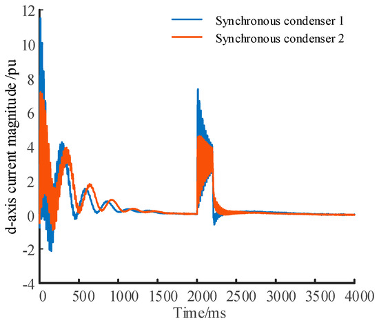
Figure 1. Reactive current of synchronous condenser with different X″_d values.

Under the transient condition, the stator voltage equation and the flux linkage equation can be obtained as [23]

$$\left\{\begin{array}{l}{v}_d=-r_s{i}_d\left(s\right)+s{\psi }_d\left(s\right)-{\psi }_{d0}-{\psi }_q\left(s\right)\\ v_q=-r_s{i}_q\left(s\right)+s{\psi }_q\left(s\right)-{\psi }_{q0}+{\psi }_d\left(s\right)\end{array}\right.$$

(5)

$$\left\{\begin{array}{l}{\psi }_d\left(s\right)=-X_d\left(s\right)i_d\left(s\right)+{\displaystyle \frac{X_{ad}{i}_{f0}}{s}}\\ {\psi }_q\left(s\right)=-X_q\left(s\right)i_q\left(s\right)\end{array}\right.$$

(6)

Taking into account all initial conditions and the absence of a damping winding, it follows that X_q(s) equals X_q. By combining (5) and (6), while accounting for the relatively small value of the stator resistance r_s, the following expression is derived:

$${\displaystyle \frac{X_{ad}{i}_{f0}}{s}}=\left[s^2+s{r}_s({\displaystyle \frac{1}{{X^{\prime }}_d}}+{\displaystyle \frac{1}{X_q}})+1\right]X_d\left(s\right)i_d\left(s\right)$$

(7)

When neglecting damping, the reciprocal of the d-axis transient reactance is represented as

$${\displaystyle \frac{1}{X_d\left(s\right)}}={\displaystyle \frac{1}{X_d}}+({\displaystyle \frac{1}{{X^{\prime }}_d}}-{\displaystyle \frac{1}{X_d}}){\displaystyle \frac{s{T^{\prime }}_d}{s{T^{\prime }}_d+1}}$$

(8)

Under no-load operation, the terminal voltage of the exciter is equal to the excitation electromotive force, i.e., X_adi_f0(s) = v_q0 = √3E₀. By combining (7) and (8), the d-axis current i_d can be obtained as

$$i_d\left(s\right)={\displaystyle \frac{\sqrt{3}{E}_0}{s\left[s^2+s{r}_s(\frac{1}{{X^{\prime }}_d}+\frac{1}{X_q})+1\right]}}·\left[{\displaystyle \frac{1}{X_d}}+({\displaystyle \frac{1}{{X^{\prime }}_d}}-{\displaystyle \frac{1}{X_d}}){\displaystyle \frac{s{T^{\prime }}_d}{s{T^{\prime }}_d+1}}\right]$$

(9)

Based on the inverse Laplace transform, the d-axis current i_d in the time domain can be obtained as

$$\left\{\begin{array}{l}{i}_d=\sqrt{3}{E}_0\left[{\displaystyle \frac{1}{X_d}}+({\displaystyle \frac{1}{{X^{\prime }}_d}}-{\displaystyle \frac{1}{X_d}})e^{-{\displaystyle \frac{t}{{T^{\prime }}_d}}}\right]-{\displaystyle \frac{\sqrt{3}{E}_0}{{X^{\prime }}_d}}{e}^{-{\displaystyle \frac{t}{T_a}}}\cos t\\ T_a={\displaystyle \frac{2{X^{\prime }}_d{X}_q}{{X^{\prime }}_d+X_q}}\end{array}\right.$$

(10)

From (10), with X_d held constant, X′_d determines the magnitude of the stator current, and T_a determines the oscillation time. Figure 2 illustrates the stator current output of two synchronous condensers during a three-phase short-circuit fault. The X′_d is 0. 165 pu for the synchronous condenser 1 and 0.30 pu for the synchronous condenser 2.

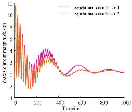
Figure 2. Reactive current of synchronous condenser with X′_d.

According to Figure 2, it is evident that condenser 2 exhibits significantly faster attenuation in both transient and sustained reactive power. As for the stability of sustained reactive power output, condenser 1 exhibits superior performance when compared to condenser 2. After the fault is cleared, condenser 1 is capable of delivering higher reactive power than condenser 2. Therefore, as X′_d decreases, condenser 1 becomes more stable and can provide more reactive power.

As aforementioned, the reactive power is primarily influenced by the d-axis parameters, whereas the q-axis parameters have minimal influence on reactive power output. Thus, when analyzing the reactive voltage of synchronous condensers, paramount focus should be allocated to the d-axis parameters under the sub-transient and transient conditions.

2.2. Introduction to the Algorithm

The trajectory sensitivity of the parameter x_i refers to the ratio between the variation in the system output variable y and the perturbation in parameter x_i [17],

$${\displaystyle \frac{\partial y\left(x_i,N\right)}{\partial x}}=\underset{\Delta x_i\to 0}{\lim }{\displaystyle \frac{1}{\Delta x_i}}·\left[y\left(x_i+\Delta x,N\right)-\right.\left.y\left(x_i,N\right)\right]$$

(11)

The sensitivity analysis method is utilized to categorize the parameters to be identified into different types and establish sets of coupling variables, which can be listed as the voltage-type parameter set (VTPS), the reactive power-type parameter set (RTPS), and the neutral-type parameter set (NTPS). The procedure of the proposed classification method can be summarized as follows:

(1) According to the limits of parameter changes, the parameters to be categorized are assigned their respective lower limit values, while keeping the remaining parameters unchanged. Subsequently, simulation trajectories of voltage and reactive power are sampled, and the corresponding errors are calculated as

$$\left\{\begin{array}{l}{E}_V=\sqrt{{\displaystyle \sum _{i=1}^N{\left(V_{t,i}-{V^{\prime }}_{t,i}\right)}^2}}\\ E_Q=\sqrt{{\displaystyle \sum _{i=1}^N{\left(Q_{e,i}-{Q^{\prime }}_{e,i}\right)}^2}}\end{array}\right.$$

(12)

(2) Conduct simulations for the next step based on the parameter adjustment. Follow these procedures to calculate voltage and reactive power errors, and record the results. Repeat step (2) until the parameter reaches its upper limit.

(3) Quantify the extent of parameter sensitivity by aggregating the absolute changes in values over a unit step, which can be expressed as

$$\left\{\begin{array}{l}{S}_{V,i}={\displaystyle \sum _{m=1}^{M-1}\left|E_{V,i,m+1}-E_{V,i,m}\right|}\\ S_{Q,i}={\displaystyle \sum _{m=1}^{M-1}\left|E_{Q,i,m+1}-E_{Q,i,m}\right|}\end{array}\right.$$

(13)

(4) By setting the deviation threshold S_T for the sensitivity indices, the parameter i can be categorized as follows: If the difference between S_V,i and S_Q,i exceeds S_T, and S_V,i is higher than S_Q,i, the parameter i belongs to VTPS. If the difference between S_V,i and S_Q,i exceeds S_T, and S_V,i is lower than S_Q,i, the parameter i belongs to RTPS. In all other cases, the parameter i belongs to NTPS.

3. Parameter Identification Model and Data Preprocess

3.1. Parameter Identification Model at Multiple Time Scales

During the operation of a synchronous condenser, both the steady-state and transient states play significant roles. The steady-state parameters have an influence on both the steady-state and transient processes of the synchronous condenser, while the transient parameters solely impact its transient operation. Therefore, the step-wise identification of steady-state and transient parameters is conducted to improve accuracy.

The identification of steady-state parameters in a synchronous condenser takes steady-state data as input and steady-state parameters as the quantities to be determined, which can be expressed as

$$\left\{\begin{array}{l}{i}_{f0}=v_{q0}+X_d{i}_{d0}\\ i_{f0}=K_c{v}_{f0}\end{array}\right.$$

(14)

$$0=\mathit{h}\left({\mathit{X}}_S,{\mathit{I}}_S\right)$$

(15)

As aforementioned, the reactive power is primarily influenced by the d-axis parameters and remains independent of the q-axis parameters. Therefore, the focus is to identify the d-axis parameters, which can be represented as

$$\left\{\begin{array}{l}{T}_{d0}^{\prime }{\displaystyle \frac{d{E}_q^{\prime }}{dt}}=-E_q^{\prime }-{\displaystyle \frac{X_d-X_d^{\prime }}{X_d^{\prime }-X_d^{″}}}(E_q^{\prime }-E_q^{″})+E_f\hfill \\ T_{d0}^{″}{\displaystyle \frac{d{E}_q^{″}}{dt}}=E_q^{\prime }-E_q^{″}-(X_d^{\prime }-X_d^{″})i_d\hfill \\ T_{q0}^{″}{\displaystyle \frac{d{E}_d^{″}}{dt}}=-E_d^{″}+(X_q-X_q^{″})i_q\hfill \\ T_a{\displaystyle \frac{d{V}_R}{dt}}=K_a(V_{ref}-V_t+V_{PSS}-V_F)-V_R\hfill \\ T_e{\displaystyle \frac{d{E}_f}{dt}}=V_R-K_e{E}_f\hfill \\ T_f{\displaystyle \frac{d{V}_F}{dt}}={\displaystyle \frac{K_f}{T_e}}(V_R-K_e{E}_f)-V_F\hfill \\ E_f=K{V}_f\hfill \\ v_q=E_q^{″}-X_d^{″}{i}_d\hfill \\ v_d=E_d^{″}+X_q^{″}{i}_q\hfill \\ V_t=\sqrt{v_q^2+v_d^2}\hfill \\ Q_e=v_q{i}_d-v_d{i}_q\hfill \end{array}\right.$$

(16)

Based on the mathematical model of the SCES and the coupling variable sets, the transient parameter identification model can be established. The objective of the parameter identification model for the VTPS is to minimize the differences between the estimated voltage and its actual value, which can be expressed as

$$\begin{array}{l}\min \sqrt{{\displaystyle \sum _{i=1}^N{\left(V_{t,i}-V_{t\_est,i}\right)}^2}}\\ \left\{\begin{array}{l}{\displaystyle \frac{d\mathit{x}}{d\mathit{t}}}=\mathit{f}\left(\mathit{x},{\mathit{X}}_V,{\mathit{I}}_Z\right)\\ 0=\mathit{g}\left(\mathit{x},{\mathit{X}}_V,{\mathit{I}}_Z\right)\end{array}\right.\end{array}$$

(17)

The objective of the parameter identification model for the RTPS is to minimize the differences between the estimated reactive power and its actual value, which can be expressed as

$$\begin{array}{l}\min \sqrt{{\displaystyle \sum _{i=1}^N{\left(Q_{e,i}-Q_{e\_est,i}\right)}^2}}\\ \left\{\begin{array}{l}{\displaystyle \frac{d\mathit{x}}{d\mathit{t}}}=\mathit{f}\left(\mathit{x},{\mathit{X}}_Q,{\mathit{I}}_Z\right)\\ 0=\mathit{g}\left(\mathit{x},{\mathit{X}}_Q,{\mathit{I}}_Z\right)\end{array}\right.\end{array}$$

(18)

The parameter identification model for the NTPS aims to minimize the sum of the differences of the voltage and reactive power, with the objective function formulated as

$$\begin{array}{l}\min \left[\sqrt{{\displaystyle \sum _{i=1}^N{\left(V_{t,i}-V_{t\_est,i}\right)}^2}}+\sqrt{{\displaystyle \sum _{i=1}^N{\left(Q_{e,i}-Q_{e\_est,i}\right)}^2}}\right]\\ \left\{\begin{array}{l}{\displaystyle \frac{d\mathit{x}}{d\mathit{t}}}=\mathit{f}\left(\mathit{x},{\mathit{X}}_N,{\mathit{I}}_Z\right)\\ 0=\mathit{g}\left(\mathit{x},{\mathit{X}}_N,{\mathit{I}}_Z\right)\end{array}\right.\end{array}$$

(19)

3.2. Data Noise Preprocessing Method

In the practical operation of power systems, the data obtained from measurements often contain noise. Prior to parameter identification, it is imperative to preprocess the noisy data to enhance the identification accuracy [23,24]. Thus, the WTD method is used to preprocess the measurement data, as illustrated in Figure 3.

Figure 3. Schematic diagram of WTD method.

The WTD method first decomposes the original signal into different scales [25,26]. The wavelet coefficients exceeding the specified threshold are deemed to be signal-generated and retained, while those falling below the threshold are considered as noise-induced and either attenuated or set to zero. The one-dimensional noisy signal f(t) is expressed as

$$f(t)=x(t)+n(t)$$

(20)

The noisy signal f(t) is decomposed using the selected wavelet basis and decomposition levels, which can be expressed as

$$W\left(j,k\right)=2^{-j/2}{\displaystyle \sum _{t=0}^{N-1}f\left(t\right)}+\psi \left(2^{-j}-k\right)j,k\in Z$$

(21)

Moreover, the Mallat method is utilized for implementing the wavelet transformation, which can be expressed as

$$S\left(j+1,k\right)=S\left(j,k\right)h_r\left(j,k\right)$$

(22)

$$W\left(j+1,k\right)=S\left(j,k\right)g_r\left(j,k\right)$$

(23)

Subsequently, the coefficients of the low-frequency approximation signal are preserved at the maximum scale, while appropriate threshold functions and thresholds are determined to effectively filter out high-frequency signal coefficients at other scales. The denoised signal is obtained by employing the low-frequency coefficients in conjunction with the estimated high-frequency coefficients for wavelet reconstruction. The process of wavelet reconstruction can be formulated as

$$S\left(j-1,k\right)=S\left(j,k\right)\ast h_g\left(j,k\right)+W\left(j,k\right)\ast g_g\left(j,k\right)$$

(24)

4. Solution Method Based on Improved SO Method

4.1. Parameter Identification Based on Coupling Variable Set

The parameter identification approach for the SCES is illustrated in Figure 4. The key parameters of the synchronous condenser are selected for identification. Furthermore, three sets of coupling variables are established based on sensitivity analysis. Additionally, a parameter identification model is developed under steady-state, sub-transient, and transient conditions. Moreover, the measurement data are preprocessed using the WTD method. The parameter identification relies on the response data of the synchronous condenser and its excitation system. Thus, the proposed approach can be utilized online to collect the response data and update the model parameter periodically.

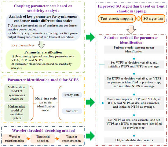
Figure 4. Schematic diagram of proposed SCES parameter identification approach.

Therefore, the procedures of the proposed SCES parameter identification approach can be listed as follows:

(1) Perform the steady-state parameter identification, utilizing post-disturbance data to calculate the d-axis steady-state parameter, while the original values of the q-axis parameters are used.

(2) Perform the parameter identification for the VTPS. Set the parameters in the VTPS as the decision variables and initialize the parameters in the RTPS and NTPS based on the averages within the parameter ranges. Identify the parameters in the VTPS by (17).

(3) Perform the parameter identification for the RTPS. Set the parameters in the RTPS as the decision variables and the parameters in the VTPS as the identification results from step (2). Initialize the parameters in the NTPS by selecting the averages within the parameter ranges, and identify the parameters in the RTPS by (18).

(4) According to the identification results from steps (2) and (3), restrict the search range of the parameters in the VTPS and RTPS. Set both the parameters in the VTPS and RTPS as decision variables, while the parameters in the NTPS are set to the averages within the parameter ranges. The optimization objective is the objective function defined by (19).

(5) Perform the parameter identification for the NTPS. Set the parameters in the NTPS as decision variables, while the parameters in the VTPS and RTPS adopt the identification results from step (4). Identify the parameters in the NTPS by (19).

The parameter identification accuracy improvement ratio is used to measure the performance, which is expressed as

$$I_E={\displaystyle \frac{E_{r,o}-E_{r,n}}{E_{r,o}}}$$

(25)

4.2. Improved SO Method Based on Tent Chaotic Mapping

The SO method, as a novel metaheuristic method, possesses excellent search capability and convergence speed. However, its initialization of the population is based on randomly generating variables within a given range, which introduces significant randomness and uncertainty [27]. In order to address this issue, the population initialization in the SO method is improved by Tent mapping to generate chaotic sequences [28,29]. The improved SO method is used to solve the parameter identification model (17)~(19). Therefore, the fitness function is set as the reciprocal of the objective function. Moreover, the sneaker individual that violates the constraints will be deleted from the population.

During the population initialization stage, Tent chaotic mapping is utilized to generate the initial position sequence for the snakes. At this stage, the initial position sequence of the snake, denoted as X_i,j, is expressed as

$$Z(t+1)=\left\{\begin{array}{ll}{\displaystyle \frac{Z(t)}{u}}& ,0\le Z(t)\le u\hfill \\ {\displaystyle \frac{1-Z(t)}{1-u}}& ,u<Z(t)\le 1\hfill \end{array}\right.$$

(26)

$$X_{i,j}=(X_{\max }-X_{\min })·Z(j)+X_{\min }$$

(27)

Once the population is initialized, the SO method simulates the process of survival and reproduction of the snake swarm. The search phase consists of the exploration and exploitation stages. In the exploration stage, when there is a scarcity of food, snakes search for food by selecting random positions, which can be expressed as

$$\left\{\begin{array}{l}{X}_{i,j}(t+1)=X_{r,j}(t)\pm c_1{A}_j\left[\left(X_{\max }-X_{\min }\right)·r+X_{\min }\right]\\ A_j=\exp ({\displaystyle \frac{-f_{r,j}}{f_{i,j}}})\end{array}\right.$$

(28)

The behavior in the exploitation stage is conducted according to temperature conditions. When the environmental temperature T is greater than or equal to the threshold T_h, snakes will solely focus on searching for food and updating their positions, which can be represented as

$$\left\{\begin{array}{l}{X}_{i,j}\left(t+1\right)=X_f\pm c_2·T·r\left[X_f-X_{i,j}\left(t\right)\right]\\ T=\exp ({\displaystyle \frac{-t}{N_m}})\end{array}\right.$$

(29)

When the temperature T is below the threshold T_h, the snakes enter either the combat or mating modes. In the combat modes, the position X_i,j can be expressed as

$$\left\{\begin{array}{l}{X}_{i,j}\left(t+1\right)=X_{i,j}(t)+c_2·F_j\left[Q_a\cdot X_{b,j}-X_{i,j}\left(t\right)\right]\\ F_j=\exp ({\displaystyle \frac{-f_{b,j}}{f_{i,j}}})\\ Q_a=c_3·\exp ({\displaystyle \frac{t-N_m}{N_m}})\end{array}\right.$$

(30)

Additionally, in the mating modes, the position X_i,j can be expressed as

$$\left\{\begin{array}{l}{X}_{i,j}\left(t+1\right)=X_{i,j}(t)+c_2·M_j·r·\left[Q_a·X_{i,j}(t)-X_{i,j}(t)\right]\hfill \\ M_m=\exp ({\displaystyle \frac{-f_{i,f}}{f_{i,m}}})\hfill \\ M_f=\exp ({\displaystyle \frac{-f_{i,m}}{f_{i,f}}})\hfill \end{array}\right.$$

(31)

5. Case Studies

The parameters of a real-world SCES are used, as shown in Table 1. MATLAB/Simulink was used for simulation, with a simulation time of 10 s. A three-phase short circuit fault is set to occur at 5 s and last for 0.2 s. The db4 wavelet is selected as the basis function for the WTD method, and a decomposition level of 3 is chosen. In addition, the environmental temperature threshold value of the improved SO method T_h is set as 0.6.

Table 1. Parameters of real-world SCES.

Parameter	Value	Parameter	Value
Xd	1.305	Xl	0.18
X′d	0.296	T′d	7.01
X″d	0.252	T″d	0.053
Xq	1.300	T″q0	0.1
X″q	0.243	Rs	0.002854
Tr	0.002	Kf	0.2
Ka	300	Tf	0.1
Ta	0.3	Efmin	−11.5
Ke	1	Efmax	11.5
Te	0.3	Kp	0
Tb	0	Vt0	1
Tc	0	Vf0	1.29

5.1. Parameter Classification and Data Preprocessing

The parameters of the SCES are classified into RTPS, NTPS, and VTPS. Taking X′_d, T′_d0, and K_a as examples, the variations in error trends concerning these parameters are illustrated in Figure 5, Figure 6 and Figure 7. From Figure 5, it can be seen that the variation in reactive power error is significantly larger compared to the voltage error as the parameter X′_d changes. An analysis of Figure 7 and Figure 8 reveals that as the parameter K_a varies, the variation in voltage error surpasses that of reactive power error. However, for the parameter T′_d0, both voltage and reactive power errors exhibit similar changes as its value varies. When both parameters K_a and T′_d0 reach their respective set values, both errors become zero.

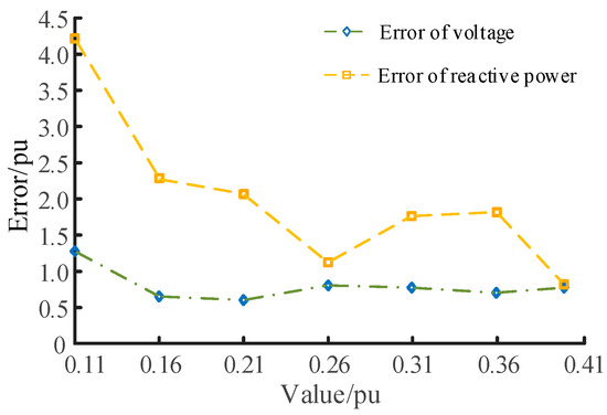
Figure 5. Variation in error with different X′_d values.

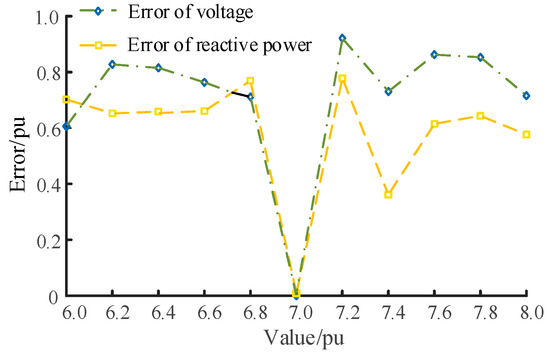
Figure 6. Variation in error with different T′_d0 values.

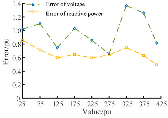
Figure 7. Variation in error with different X′_d values.

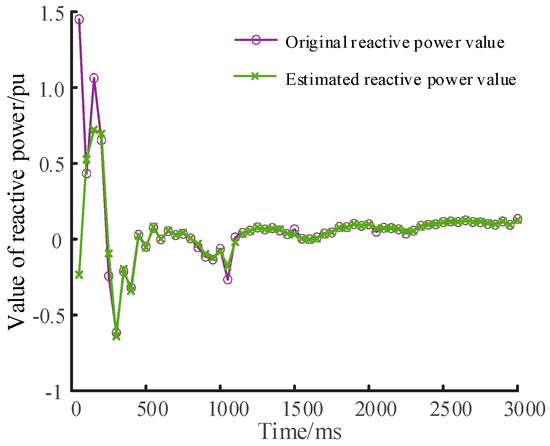
Figure 8. Reactive power response without WTD method.

Based on the aforementioned analysis, Table 2 presents the sensitivity indices. The threshold for the voltage and reactive power sensitivity is set as 0.1. And the classification results are displayed in Table 3. In Table 2, the parameter X′_d exhibits a higher S_Q compared to S_V, thus categorizing it as RTP. Similarly, the parameter K_a falls under VTPS classification. Moreover, the discrepancy between S_Q and S_V for parameter Tʹ_d0 is merely 0.041, so its parameter type is NTPS.

Table 2. Sensitivity of parameters to voltage and reactive power.

Parameter	Voltage Sensitivity SV	Reactive Power Sensitivity SQ	Parameter	Voltage Sensitivity SV	Reactive Power Sensitivity SQ
X′d	2.6044	7.0363	Ta	2.0662	2.4714
X″d	3.7357	3.5789	Kf	2.6348	3.0097
T′d0	2.4388	2.4798	Tf	4.4414	3.1904
T″d0	3.3031	1.7630	Ke	2.5640	1.3667
Ka	3.6715	2.0412	Te	3.2497	1.6479

Table 3. Classification of parameters to be identified.

Parameter	Type	Parameter	Type
X′d	RTPS	Ta	RTPS
X″d	VTPS	Kf	RTPS
T′d0	NTPS	Tf	VTPS
T″d0	VTPS	Ke	VTPS
Ka	VTPS	Te	VTPS

To demonstrate the impact of the WTD method on identification accuracy, the difference in estimated reactive power is analyzed. The response of reactive power is depicted in Figure 8 and Figure 9 for cases without and with the WTD method, respectively. The effectiveness of the WTD method in mitigating estimation error is clearly evident.

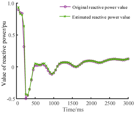
Figure 9. Reactive power response with WTD method.

5.2. Comparative Analysis of Parameter Identification Error

A comparative analysis of parameter identification error is conducted. In Scheme 1, simultaneous identification of all parameters is performed without classification. The corresponding results of steady-state and transient parameters are presented in Table 4 and Table 5, respectively.

Table 4. Identification results of steady-state parameters.

Parameter	Real Value	Identification Result	Identification Error
Xd	1.305	1.3137	0.667%
K	0.998	1.0012	0.321%

Table 5. Identification results of transient parameters.

Type	Parameter	Real Value	Scheme 1	Identification Error	Proposed Approach	Identification Error
VTPS	X″d	0.252	0.263	0.56%	0.252	0.08%
	T″d0	0.053	0.064	5.66%	0.053	0.76%
	Ka	300	293.87	2.04%	296.73	1.09%
	Tf	0.1	0.090	3.90%	0.108	7.80%
	Ke	1	0.900	9.99%	1.030	3.04%
	Te	0.3	0.278	7.27%	0.319	6.50%
RTPS	X′d	0.296	0.306	3.38%	0.290	1.96%
	Ta	0.3	0.315	5.03%	0.301	0.17%
	Kf	0.2	0.204	2.15%	0.196	2.25%
NTPS	T′d0	7.01	6.013	14.2%	6.890	1.71%

Under the steady-state condition, both identification methods employ the same calculation process. The maximum identification error is 0.667%, which falls within an acceptable range. For transient parameters, the proposed approach exhibits lower errors compared to Scheme 1, as demonstrated in Table 5. However, for certain parameters such as T_f and K_f, their numerical values are relatively small, and the precision limitations of the solution method restrict the obtained results. Nevertheless, these numerical differences still remain within an acceptable range.

To quantify the superiority of the proposed approach, the improvement ratio for parameter identification accuracy I_E is calculated using Equation (25). Table 6 presents a comparison between the proposed approach and Scheme 1, listing the I_E for each parameter in the proposed approach.

Table 6. Improvement ratio for parameter identification accuracy of proposed approach.

Parameter	Improvement Ratio IE	Parameter	Improvement Ratio IE
X′d	0.420	Ta	0.967
X″d	0.867	Kf	−0.047
T′d0	0.880	Tf	−1.000
T″d0	0.867	Ke	0.696
Ka	0.467	Te	0.106

From Table 6, it can be seen that the identification accuracy has improved by the proposed approach for all parameters except for T_f and K_f, when compared to Scheme 1. Among these parameters, T_a exhibits the most significant enhancement with a remarkable increase in accuracy by 42.23%. These results show the effectiveness of the proposed approach in reducing parameter identification errors.

5.3. Comparative Analysis of Reactive Power and Voltage Response

The comparative analysis of the dynamic response error of the proposed approach and Scheme 1 is conducted. The simulation time is set as 6 s, during which a three-phase short circuit fault occurs at 2 s and is cleared at 0.2 s The corresponding response trajectories of voltage and reactive power can be illustrated in Figure 10 and Figure 11, respectively.

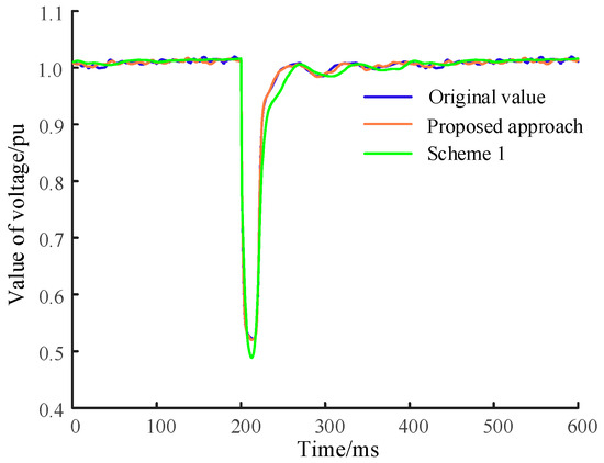
Figure 10. Voltage dynamic response of different methods.

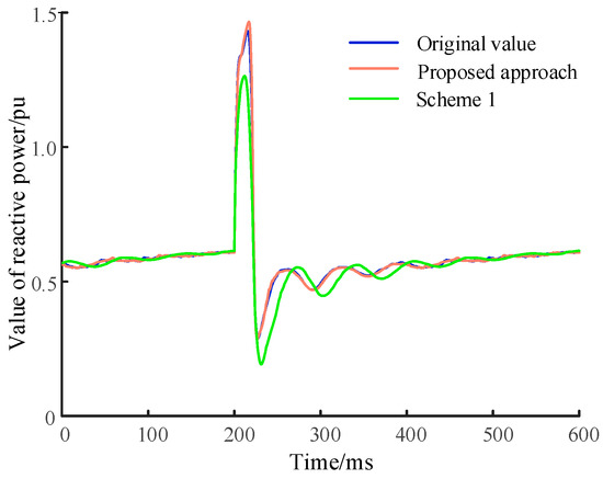
Figure 11. Reactive power dynamic response of different methods.

The dynamic response trajectories of the proposed approach exhibit a higher level of consistency with the original trajectories, as demonstrated in Figure 10 and Figure 11. Scheme 1 identifies both X′_d and X″_d as higher than their original values, indicating a weaker reactive power support capability at fault occurrence, consequently resulting in a more pronounced voltage drop.

Furthermore, the root mean square error (RMSE) is utilized to quantify the dynamic response error. The calculated RMSE values are presented in Table 7, revealing that the proposed approach exhibits significantly smaller RMSEs for voltage and reactive power compared to Scheme 1. Specifically, the proposed approach achieves remarkable reductions of 62.94% in voltage RMSE and 83.73% in reactive power RMSE. These results not only validate the advantages of the proposed approach but also highlight its high practical significance.

Table 7. RMSE of voltage and reactive power.

Method	RMES of Voltage	RMES of Reactive Power
Scheme 1	0.0340	0.0510
Proposed approach	0.0126	0.0083

6. Conclusions

A parameter identification approach is proposed for the SCES parameters considering multivariate coupling characteristics. The key parameters of the synchronous condenser are selected for identification, and a sensitivity analysis method is employed to classify the parameters and establish coupling variable sets. Subsequently, a multi-time-scale parameter identification model is developed, utilizing both the WTD method and the improved SO method for solution. The case study results demonstrate the superior performance of the proposed approach in enhancing the parameter identification accuracy while reducing the errors in reactive power and voltage dynamic response. The voltage RMSE and reactive power RMSE of the proposed approach can be reduced by 62.94% and 83.73%, respectively.

Therefore, the main contributions are listed as follows:

(1) The key parameters of the synchronous condenser are selected for identification through the analysis of the factors that influence its reactive power output.

(2) The parameters of the SCES to be identified can be classified by the trajectory sensitivity, on which three sets of coupling variables are established.

(3) A multi-time-scale parameter identification model is developed for the SCES, taking into account the steady-state, sub-transient, and transient conditions.

(4) The noise of measurement data is processed by the WTD method, and an improved SO method based on Tent chaotic mapping is proposed for a solution.

In future works, an optimal control strategy for a synchronous condenser will be presented based on the identified model parameters.

References

- Zhang, J.; Wang, J.; Cao, Y.; Li, B.; Li, C. A coordinated control strategy of multi-type flexible resources and under-frequency load shedding for active power balance. Symmetry 2024, 16, 479. [Google Scholar] [CrossRef]
- Cao, Y.; Wu, Q.; Li, C.; Jiao, W.; Tan, J. Chance-constrained optimal sizing of BESS with emergency load shedding for frequency stability. Appl. Energy 2024, 367, 123455. [Google Scholar] [CrossRef]
- Wang, W.; Li, G.; Guo, J. Large-scale renewable energy transmission by HVDC: Challenges and proposals. Engineering 2022, 19, 252–267. [Google Scholar] [CrossRef]
- Chen, X.; Wu, P.; He, H.; Song, B.; Qin, K.; Teng, X.; Yang, F.; Li, D. Optimal flexibility dispatching of multi-pumped hydro storage stations considering the uncertainty of renewable energy. Symmetry 2024, 16, 1404. [Google Scholar] [CrossRef]
- Zhang, J.; Ma, R.; Cao, Y.; Zou, S.; Li, C. Quantitative assessment of static voltage stability for power system with high-penetration wind power based on energy function. Energy Rep. 2024, 12, 699–707. [Google Scholar] [CrossRef]
- Jiang, M.; Ma, H.; Zhang, Y.; Chen, X.; Zhao, X. Reactive power characteristics and vibration properties under SISC in synchronous condensers. Int. J. Electr. Power Energy Syst. 2021, 133, 107318. [Google Scholar] [CrossRef]
- Jawad, A. A systematic approach to estimate the frequency support from large-scale PV plants in a renewable integrated grid. Energy Rep. 2022, 8, 940–954. [Google Scholar] [CrossRef]
- Zimmer, V.; Decker, I.C.; ESilva, A.S. A robust approach for the identification of synchronous machine parameters and dynamic states based on PMU data. Electr. Power Syst. Res. 2018, 165, 167–178. [Google Scholar] [CrossRef]
- Oteafy AM, A.; Chiasson, J.N.; Ahmed-Zaid, S. Development and application of a standstill parameter identification technique for the synchronous generator. Int. J. Electr. Power Energy Syst. 2016, 81, 222–231. [Google Scholar] [CrossRef]
- Xiao, Q.; Liao, K.; Shi, C.; Zhang, Y. Parameter identification of direct-drive permanent magnet synchronous generator based on EDMPSO-EKF. IET Renew. Power Gener. 2022, 16, 1073–1086. [Google Scholar] [CrossRef]
- Arastou, A.; Karrari, M.; Zaker, B. New method for synchronous generator parameters estimation using load rejection tests data considering operational limitations. Electr. Power Syst. Res. 2021, 192, 106999. [Google Scholar] [CrossRef]
- Zaker, B.; Khodadadi, A.; Karrari, M. A new approach to parameter identification of generation unit equipped with brushless exciter using estimated field voltage. Int. J. Electr. Power Energy Syst. 2022, 141, 108122. [Google Scholar] [CrossRef]
- Wang, Z.; Chai, J.; Xiang, X.; Sun, X.; Lu, H. A novel online parameter identification method designed for deadbeat current control of the permanent-magnet synchronous motor. IEEE Trans. Ind. Appl. 2021, 58, 2029–2041. [Google Scholar] [CrossRef]
- Micev, M.; Ćalasan, M.; Aleem, S.H.; Hasanien, H.M.; Petrović, D.S. Two novel approaches for identification of synchronous machine parameters from short-circuit current waveform. IEEE Trans. Ind. Electron. 2021, 69, 5536–5546. [Google Scholar] [CrossRef]
- Zhang, F.; Liu, J. Parameter identification with synchrophasor trajectory fitting technique for sub-/super-synchronous oscillations. IEEE Trans. Power Syst. 2022, 37, 3181–3184. [Google Scholar] [CrossRef]
- Li, X.; Kennel, R. General formulation of Kalman-filter-based online parameter identification methods for VSI-fed PMSM. IEEE Trans. Ind. Electron. 2020, 68, 2856–2864. [Google Scholar] [CrossRef]
- Guo, Q.; Gao, L.; Chu, X.; Sun, H. Parameter identification for static var compensator model using sensitivity analysis and improved whale optimization method. CSEE J. Power Energy Syst. 2022, 8, 535–547. [Google Scholar]
- Chen, C.; Li, C.; Liao, C.; Wang, L. Parameter identification of capacitive power transfer system based on spectrum analysis. CPSS Trans. Power Electron. Appl. 2018, 3, 181–186. [Google Scholar] [CrossRef]
- Guddanti, B.; Orrego, J.R.; Roychowdhury, R.; Illindala, M.S. Sensitivity analysis based identification of key parameters in the dynamic model of a utility-scale solar PV plant. IEEE Trans. Power Syst. 2021, 37, 1340–1350. [Google Scholar] [CrossRef]
- Wang, A.; Zheng, Z.; Zheng, J. Parameter identification of synchronous condenser based on sensitivity analysis of parameters. In Proceedings of the 2017 China International Electrical and Energy Conference (CIEEC), Beijing, China, 25–27 October 2017; pp. 725–730. [Google Scholar]
- Zaker, B.; Gharehpetian, G.B.; Karrari, M.; Moaddabi, N. Simultaneous parameter identification of synchronous generator and excitation system using online measurements. IEEE Trans. Smart Grid 2015, 7, 1230–1238. [Google Scholar] [CrossRef]
- Kimbark E, W. Power System Stability; John Wiley & Sons: Hoboken, NJ, USA, 1995. [Google Scholar]
- Kyriakides, E.; Heydt, G.T.; Vittal, V. On-line estimation of synchronous generator parameters using a damper current observer and a graphic user interface. IEEE Trans. Energy Convers. 2004, 19, 499–507. [Google Scholar] [CrossRef]
- Mitra, A.; Mohapatra, A.; Chakrabarti, S.; Sarkar, S. Online measurement based joint parameter estimation of synchronous generator and exciter. IEEE Trans. Energy Convers. 2020, 36, 820–830. [Google Scholar] [CrossRef]
- Desai, J.P.; Makwana, V.H. A novel out of step relaying method based on wavelet transform and a deep learning machine model. Prot. Control. Mod. Power Syst. 2021, 6, 1–12. [Google Scholar] [CrossRef]
- Zhao, W.; Shang, L.; Sun, J. Power quality disturbance classification based on time-frequency domain multi-feature and decision tree. Prot. Control. Mod. Power Syst. 2019, 4, 27. [Google Scholar] [CrossRef]
- Hashim, F.A.; Hussien, A.G. Snake Optimizer: A novel meta-heuristic optimization method. Knowl.-Based Syst. 2022, 242, 108320. [Google Scholar] [CrossRef]
- Zhu, C.; Sun, K. Cryptanalyzing and improving a novel color image encryption method using RT-enhanced chaotic tent maps. IEEE Access 2018, 6, 18759–18770. [Google Scholar] [CrossRef]
- He, S.; Fu, L.; Lu, Y.; Wu, X.; Wang, H.; Sun, K. Analog circuit of a simplified Tent map and its application in sensor position optimization. IEEE Trans. Circuits Syst. II Express Briefs 2022, 70, 885–888. [Google Scholar] [CrossRef]
Disclaimer/Publisher’s Note: The statements, opinions and data contained in all publications are solely those of the individual author(s) and contributor(s) and not of MDPI and/or the editor(s). MDPI and/or the editor(s) disclaim responsibility for any injury to people or property resulting from any ideas, methods, instructions or products referred to in the content. |
© 2024 by the authors. Licensee MDPI, Basel, Switzerland. This article is an open access article distributed under the terms and conditions of the Creative Commons Attribution (CC BY) license (https://creativecommons.org/licenses/by/4.0/).