
Dynamical Complexity of Modified Leslie–Gower Predator–Prey Model Incorporating Double Allee Effect and Fear Effect


Abstract
1. Introduction
2. Mathematical Model
Positivity and Boundedness
- To prove this, we start by integrating the equations in system (5) under the initial conditions and to obtain the solution . So, system (5)’s solution can be expressed asTherefore, we can conclude that every solution starting in the interior of set , that is, , remains in for . Along with this, for all future time, any solution trajectory that starts from the positive x-axis (or y-axis) will remain on it. Hence, the set is an invariant set.
- Under the initial conditions and , if represents any solution of the system, then we have two cases:Case 1: Let us suppose and we make the claim that . Otherwise, there will exist such that , , and ∀. Then, Equation (6) can be written asas ∀, which is a contradiction to our hypothesis. Thus, for all .Case 2: Now, let us suppose ; then, as long as ,as for .Hence, based on these two cases, we can deduce that every positive solution satisfies ∀.Next, we proceed to the predator equation of system (5):So, we have ∀, which completes our proof.
3. Existence of Equilibrium Points and Local Stability
- Axial: along with the origin, that is, , system (5) exhibits three other axial equilibrium points: , , and .
- Interior: The abscissa and ordinate of the interior equilibria can be acquired by solving the subsequent equations:The ordinate of the interior equilibrium points is given by (9). The discriminant of Equation (8) is . For the ease of calculation, consider ,, and , where . For the feasibility of positive equilibrium points, we must have , , and . Under these conditions, system (5) exhibits the following:
- Two equilibrium points and if , where , , , and .
- A unique equilibrium point if , where and .
- No equilibrium point if .
- The eigenvalues at point are and , which clearly indicate that is a saddle.
- The eigenvalues at point are − and , which clearly indicate that is an asymptotically stable point.
- The eigenvalues at point are and , which clearly indicate that is a saddle, as .
- The eigenvalues at point are and , which clearly indicate that is an unstable point, as .
- a.
- A saddle node when holds.
- b.
- A cusp of codimension two when , , and holds.
- a.
- If , then and . This implies that one eigenvalue of the Jacobian matrix is zero, while the other is non-zero, which indicates that is a saddle node.
- b.
- If , then system (11) reduces toIntroducing variables , system (12) becomeswhere , , and .Taking and , system (13) converts towhere and .Consider the transformation and ; system (14) then reduces toConsider the final transformation , and; then, system (15) reduces to
4. Bifurcation Analysis
4.1. Saddle-Node Bifurcation
4.2. Hopf Bifurcation
4.3. Bogdanov–Takens Bifurcation
- 1.
- The saddle-node bifurcation curve:;
- 2.
- The Hopf bifurcation curve:;
- 3.
- The homoclinic bifurcation curve:.
- Taking and , system (22) turns out to bewhere , ,
- Consider , , and ; then, system (27) becomeswhere , , , and ; furthermore, is a power series in with powers and satisfying , and the coefficients smoothly depend upon and .
- The saddle-node bifurcation curve ;
- The Hopf bifurcation curve ;
- The homoclinic bifurcation curve .
5. Numerical Simulation
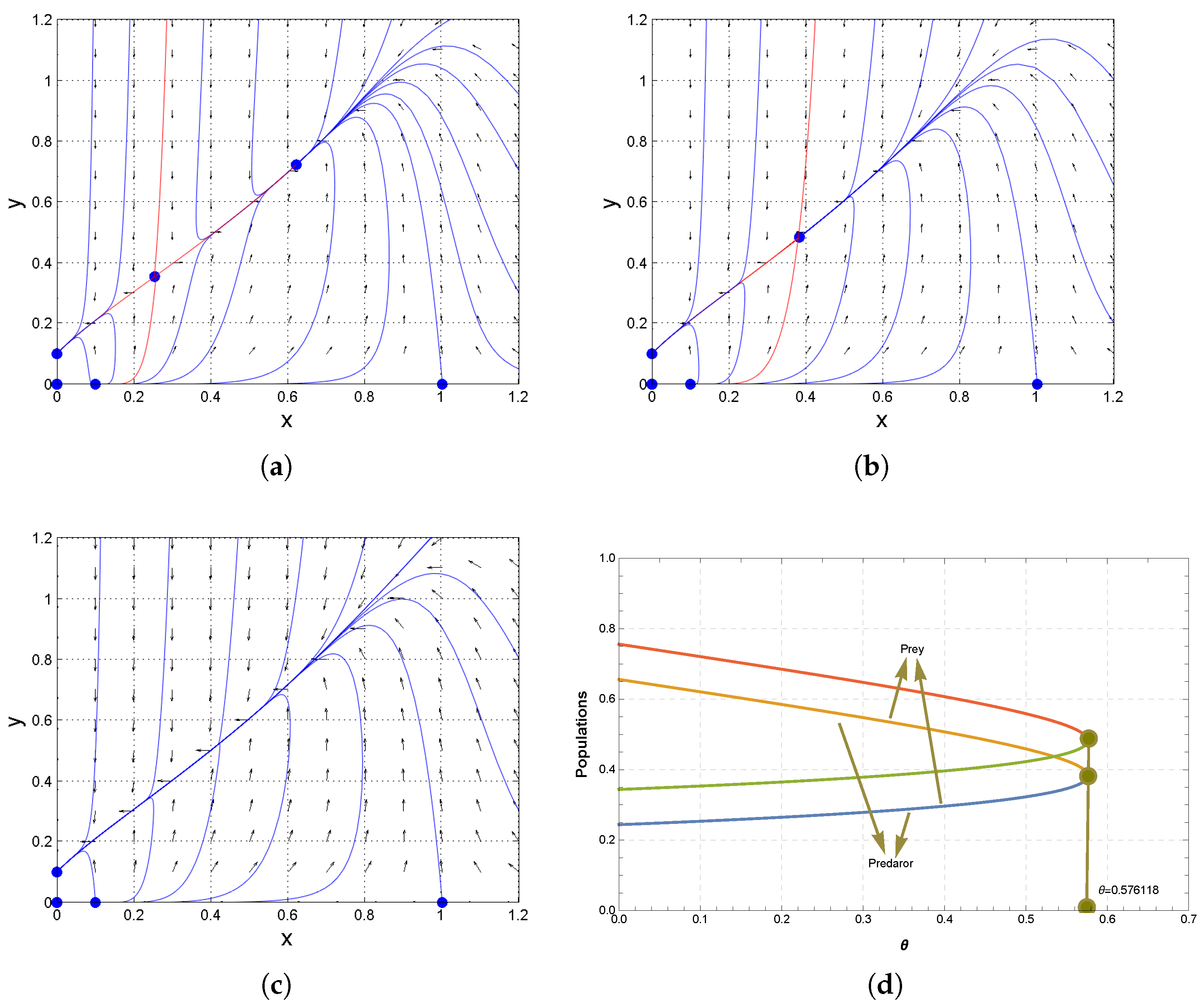
- We fixed the parameters as , , , , and in system (5). The acquired results are presented in Table 1.Table 1. Number and characteristics of equilibria that resulted from the emergence of a saddle-node bifurcation.Table 1. Number and characteristics of equilibria that resulted from the emergence of a saddle-node bifurcation.
Equilibrium Points (Stability) Figure Axial Interior (saddle) (stable), (saddle) Figure 1a (stable) (degenerate singularity), emergence of saddle-node bifurcation Figure 1b,d (unstable), (saddle) None Figure 1c Figure 1. Existence of equilibrium points. (a) At . (b) At . (c) At . The blue and red (separatrix) curves represent the solution trajectories of the system 5 and the arrows depict the direction of these trajectories in (a–c). (d) Saddle-node bifurcation diagram (upper and lower curves represent stable equilibria and unstable equilibria, respectively).Figure 1. Existence of equilibrium points. (a) At . (b) At . (c) At . The blue and red (separatrix) curves represent the solution trajectories of the system 5 and the arrows depict the direction of these trajectories in (a–c). (d) Saddle-node bifurcation diagram (upper and lower curves represent stable equilibria and unstable equilibria, respectively).![Symmetry 16 01552 g001]()
- Fixing the parameters as , , , and in (22), we first found the threshold values, which come out to be and . Corresponding to these parameters, system (5) exhibited a unique equilibrium point . By incorporating all the specified parameters, we derived the subsequent system:To transfer this equilibrium point to the origin, we made the transformations and . Then, we made the affine transformations and . So, the system reduced towhere , , , , , , , , , and ; furthermore, and were power series in with powers and satisfying , and the coefficients had a smooth dependence upon and .Next, we performed the transformations and We made a change in the time variable and rewrote T as t. Then, using the transformations and , system (37) is reduced towhere , , , , and ; furthermore, was a power series in with powers and satisfying , and the coefficients smoothly depended upon and .When and were very small, then . Now, we first considered , , and ; then, we used and . Then, making a change in the variables , , and , the system reduced towhere, , and ; furthermore, was a power series in with powers and that satisfied , and the coefficients smoothly depended upon and .

6. Impact of Fear Effect
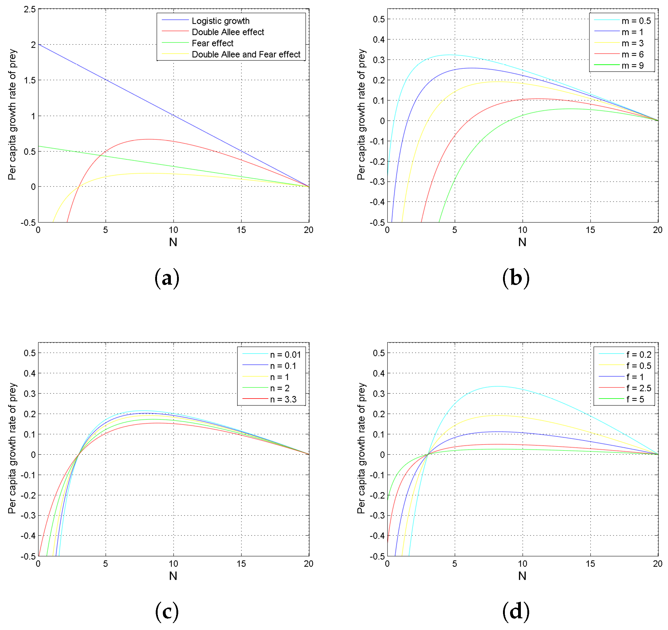
- Consider the prey equation of model (4) while the predator was taken as a constant. In this scenario, model (4) is reduced toIn reality, this scenario where the predators remain constant in an environment is highly unlikely, but there do exist some cases in which keeping a species’ population constant is possible, and this allows us to control the dynamics of an ecological system to some extent. To fulfill the aim of this study, the predator species was considered constant so that the impact of the fear effect could be explored at great length. Since fear is a feeling that is induced in prey due to the presence of predators only, we cannot disregard the existence of predators even while doing a study on just the growth function of the prey.In addition to the fear effect, we also considered the influence of the double Allee effect on the growth rate of prey species. This purpose could be served by plotting the per capita growth rate of the prey, i.e., against the population of the prey N (see Figure 4). From Figure 4a, we can see that the incorporation of phenomena like the double Allee effect and the fear effect led to a decline in the growth rate of the prey species. Figure 4b–d reflects that as the values of the parameters m, n, and f increased, respectively, the per capita growth rate of prey species decreased. The prey population possessed a threshold value for these parameters, which was crucial in determining the extinction or survival of the species.Consider , , and ; then, system (41) reduces to the following non-dimensional form:where , , , , and .Except , system (42) has non-trivial equilibrium points given bywhere , , and . If any one of the conditions , ; , ; or , holds, then by Descartes’ sign rule, it is clear that (43) has a negative root. Let this root be , . Dividing (43) by , we obtain the following quadratic equation:Taking , the ensuing outcome is described in the following theorem.Theorem 7.
- (a)
- Two equilibrium points and when , where and ;
- (b)
- One equilibrium point when , where ;
- (c)
- No equilibrium point when .
The stability of system (42) can be determined by the sign of at various equilibrium points [46]. Differentiating given in Equation (42), we obtainThe theorem stated below and Figure 5 show the stability of system (42).Theorem 8.(a) The trivial equilibrium point is always stable, as .- (b)
- The equilibrium points , , and , if they exist, are unstable when , stable when , and semi-stable (saddle-node bifurcation), respectively.
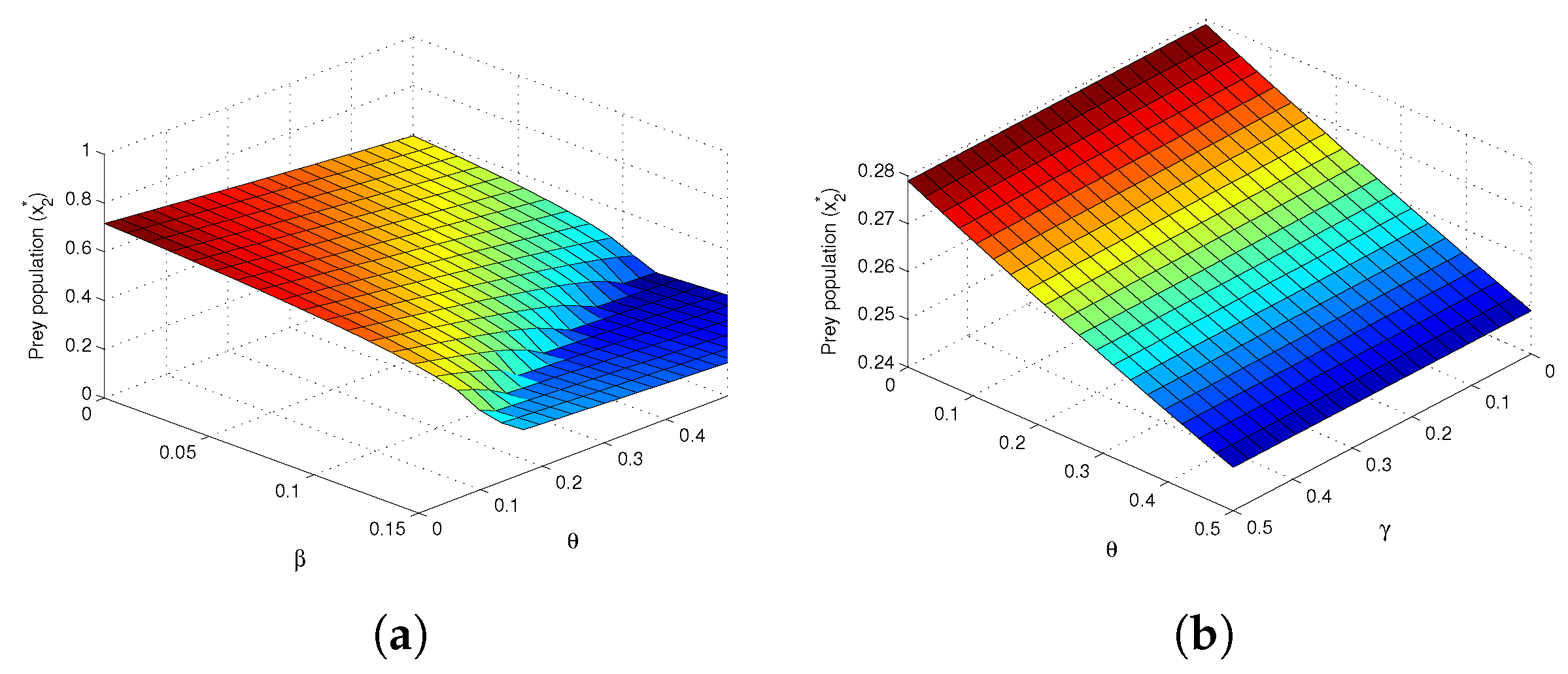
- Now, coming back to the original system (5), we present the influence of fear and the double Allee effect. Figure 6a–c illustrate that as the Allee effect parameters ( and ) and fear effect parameter (), respectively, were increased, the equilibrium point moved downward. This implies that an increase in the double Allee effect parameters and the fear effect led to the existence of an equilibrium point at a lower population. As soon as the critical value of these parameters was crossed, the system moved toward the prey-free equilibrium, which is stable in nature.Now, to observe the collective influence of the fear effect and the double Allee effect, 3D phase portraits were used. Figure 7a shows the behavior of the prey population at the stable equilibrium point against the parameters and , and it can be seen that the prey population decreased as the values of the parameters and increased. Similarly, Figure 7b reflects the same result with respect to the parameters and . Now, we know that = , which implies the predator population will also behave in the same way as the prey population regarding the parameters and , as well as and . From this, we could conclude that the higher the fear and value of the Allee effect parameters, the lower the population where system (5) attained stability. Ecologically, one can infer that escalation in the fear effect leads to a decline in prey and predator populations. As this fear intensifies, the prey population indulges less in foraging, and their interaction with each other decreases, which ultimately leads to a lower reproduction rate and, consequently, a reduced overall population. The diminishing predator–prey interaction is attributed to a declining prey population, which results in a decline in the population of predators. The populations of both species drop to the point where prey go extinct and predators survive (due to the presence of additional food).
7. Discussion
Author Contributions
Funding
Data Availability Statement
Acknowledgments
Conflicts of Interest
References
- Lotka, A.J. Elements of Physical Biology; Williams & Wilkins: Baltimore, MD, USA, 1925. [Google Scholar]
- Volterra, V. Fluctuations in the abundance of a species considered mathematically. Nature 1926, 118, 558–560. [Google Scholar] [CrossRef]
- Leslie, P.; Gower, J. The properties of a stochastic model for the predator-prey type of interaction between two species. Biometrika 1960, 47, 219–234. [Google Scholar] [CrossRef]
- Aziz-Alaoui, M.; Okiye, M.D. Boundedness and global stability for a predator-prey model with modified Leslie-Gower and Holling-type II schemes. Appl. Math. Lett. 2003, 16, 1069–1075. [Google Scholar] [CrossRef]
- Zhu, Y.; Wang, K. Existence and global attractivity of positive periodic solutions for a predator–prey model with modified Leslie–Gower Holling-type II schemes. J. Math. Anal. Appl. 2011, 384, 400–408. [Google Scholar] [CrossRef]
- Ji, C.; Jiang, D.; Shi, N. Analysis of a predator–prey model with modified Leslie–Gower and Holling-type II schemes with stochastic perturbation. J. Math. Anal. Appl. 2009, 359, 482–498. [Google Scholar] [CrossRef]
- Jiang, G.; Lu, Q.; Qian, L. Complex dynamics of a Holling type II prey–predator system with state feedback control. Chaos Solitons Fractals 2007, 31, 448–461. [Google Scholar] [CrossRef]
- Arancibia-Ibarra, C.; Flores, J. Dynamics of a Leslie–Gower predator–prey model with Holling type II functional response, Allee effect and a generalist predator. Math. Comput. Simul. 2021, 188, 1–22. [Google Scholar] [CrossRef]
- Nindjin, A.; Aziz-Alaoui, M.; Cadivel, M. Analysis of a predator–prey model with modified Leslie–Gower and Holling-type II schemes with time delay. Nonlinear Anal. Real World Appl. 2006, 7, 1104–1118. [Google Scholar] [CrossRef]
- Song, X.; Li, Y. Dynamic behaviors of the periodic predator–prey model with modified Leslie-Gower Holling-type II schemes and impulsive effect. Nonlinear Anal. Real World Appl. 2008, 9, 64–79. [Google Scholar] [CrossRef]
- Gupta, R.; Chandra, P. Bifurcation analysis of modified Leslie–Gower predator–prey model with Michaelis–Menten type prey harvesting. J. Math. Anal. Appl. 2013, 398, 278–295. [Google Scholar] [CrossRef]
- Allee, W.C. Co-operation among animals. Am. J. Sociol. 1931, 37, 386–398. [Google Scholar] [CrossRef]
- Dennis, B. Allee effects: Population growth, critical density, and the chance of extinction. Nat. Resour. Model. 1989, 3, 481–538. [Google Scholar] [CrossRef]
- Lewis, M.A.; Kareiva, P. Allee dynamics and the spread of invading organisms. Theor. Popul. Biol. 1993, 43, 141–158. [Google Scholar] [CrossRef]
- Courchamp, F.; Berec, L.; Gascoigne, J. Allee Effects in Ecology and Conservation; OUP Oxford: New York, NY, USA, 2008. [Google Scholar]
- Angulo, E.; Roemer, G.W.; Berec, L.; Gascoigne, J.; Courchamp, F. Double Allee effects and extinction in the island fox. Conserv. Biol. 2007, 21, 1082–1091. [Google Scholar] [CrossRef] [PubMed]
- Berec, L.; Angulo, E.; Courchamp, F. Multiple Allee effects and population management. Trends Ecol. Evol. 2007, 22, 185–191. [Google Scholar] [CrossRef]
- González-Olivares, E.; Mena-Lorca, J.; Rojas-Palma, A.; Flores, J.D. Dynamical complexities in the Leslie–Gower predator–prey model as consequences of the Allee effect on prey. Appl. Math. Model. 2011, 35, 366–381. [Google Scholar] [CrossRef]
- Cai, Y.; Zhao, C.; Wang, W.; Wang, J. Dynamics of a Leslie–Gower predator–prey model with additive Allee effect. Appl. Math. Model. 2015, 39, 2092–2106. [Google Scholar] [CrossRef]
- Feng, P.; Kang, Y. Dynamics of a modified Leslie–Gower model with double Allee effects. Nonlinear Dyn. 2015, 80, 1051–1062. [Google Scholar] [CrossRef]
- Pal, P.J.; Saha, T. Qualitative analysis of a predator–prey system with double Allee effect in prey. Chaos Solitons Fractals 2015, 73, 36–63. [Google Scholar] [CrossRef]
- Singh, M.K.; Bhadauria, B.; Singh, B.K. Bifurcation analysis of modified Leslie-Gower predator-prey model with double Allee effect. Ain Shams Eng. J. 2018, 9, 1263–1277. [Google Scholar] [CrossRef]
- Rahmi, E.; Darti, I.; Suryanto, A.; Trisilowati. A modified Leslie–Gower model incorporating Beddington–DeAngelis functional response, double Allee effect and memory effect. Fractal Fract. 2021, 5, 84. [Google Scholar] [CrossRef]
- Wang, F.; Yang, R.; Zhang, X. Turing patterns in a predator–prey model with double Allee effect. Math. Comput. Simul. 2024, 220, 170–191. [Google Scholar] [CrossRef]
- Yin, W.; Li, Z.; Chen, F.; He, M. Modeling Allee Effect in the Leslie-Gower Predator–Prey System Incorporating a Prey Refuge. Int. J. Bifurc. Chaos 2022, 32, 2250086. [Google Scholar] [CrossRef]
- Cruz, R.L. Stability of a Leslie-Gower type predator-prey model with a strong Allee effect with delay. Sel. Mat. 2022, 9, 24–33. [Google Scholar] [CrossRef]
- Wang, F.; Yang, R. Dynamics of a delayed reaction–diffusion predator–prey model with nonlocal competition and double Allee effect in prey. Int. J. Biomath. 2023, 2350097. [Google Scholar] [CrossRef]
- Liu, Y.; Zhang, Z.; Li, Z. The Impact of Allee Effect on a Leslie–Gower Predator–Prey Model with Hunting Cooperation. Qual. Theory Dyn. Syst. 2024, 23, 88. [Google Scholar] [CrossRef]
- Lima, S.L. Nonlethal effects in the ecology of predator-prey interactions. Bioscience 1998, 48, 25–34. [Google Scholar] [CrossRef]
- Creel, S.; Christianson, D. Relationships between direct predation and risk effects. Trends Ecol. Evol. 2008, 23, 194–201. [Google Scholar] [CrossRef]
- Cresswell, W. Predation in bird populations. J. Ornithol. 2011, 152, 251–263. [Google Scholar] [CrossRef]
- Preisser, E.L.; Bolnick, D.I. The many faces of fear: Comparing the pathways and impacts of nonconsumptive predator effects on prey populations. PLoS ONE 2008, 3, e2465. [Google Scholar] [CrossRef]
- Wang, X.; Zanette, L.; Zou, X. Modelling the fear effect in predator–prey interactions. J. Math. Biol. 2016, 73, 1179–1204. [Google Scholar] [CrossRef] [PubMed]
- Sarkar, K.; Khajanchi, S. Impact of fear effect on the growth of prey in a predator-prey interaction model. Ecol. Complex. 2020, 42, 100826. [Google Scholar] [CrossRef]
- Li, Y.; He, M.; Li, Z. Dynamics of a ratio-dependent Leslie–Gower predator–prey model with Allee effect and fear effect. Math. Comput. Simul. 2022, 201, 417–439. [Google Scholar] [CrossRef]
- Chen, M.; Takeuchi, Y.; Zhang, J.F. Dynamic complexity of a modified Leslie–Gower predator–prey system with fear effect. Commun. Nonlinear Sci. Numer. Simul. 2023, 119, 107109. [Google Scholar] [CrossRef]
- Wu, H.; Li, Z.; He, M. Dynamic analysis of a Leslie-Gower predator-prey model with the fear effect and nonlinear harvesting. Math. Biosci. Eng. 2023, 20, 18592–18629. [Google Scholar] [CrossRef]
- Al-Momen, S.; Naji, R.K. The dynamics of modified Leslie-Gower predator-prey model under the influence of nonlinear harvesting and fear effect. Iraqi J. Sci 2022, 63, 259–282. [Google Scholar] [CrossRef]
- Vinoth, S.; Vadivel, R.; Hu, N.T.; Chen, C.S.; Gunasekaran, N. Bifurcation Analysis in a Harvested Modified Leslie–Gower Model Incorporated with the Fear Factor and Prey Refuge. Mathematics 2023, 11, 3118. [Google Scholar] [CrossRef]
- Jamil, A.R.M.; Naji, R.K. Modeling and Analysis of the Influence of Fear on the Harvested Modified Leslie–Gower Model Involving Nonlinear Prey Refuge. Mathematics 2022, 10, 2857. [Google Scholar] [CrossRef]
- Halder, S.; Bhattacharyya, J.; Pal, S. Comparative studies on a predator–prey model subjected to fear and Allee effect with type I and type II foraging. J. Appl. Math. Comput. 2020, 62, 93–118. [Google Scholar] [CrossRef]
- Purnomo, A.S.; Darti, I.; Suryanto, A.; Kusumawinahyu, W.M. Fear Effect on a Modified Leslie-Gower Predator-Prey Model with Disease Transmission in Prey Population. Eng. Lett. 2023, 31. [Google Scholar]
- Qi, H.; Meng, X. Dynamics of a stochastic predator-prey model with fear effect and hunting cooperation. J. Appl. Math. Comput. 2023, 69, 2077–2103. [Google Scholar] [CrossRef]
- Pal, D.; Kesh, D.; Mukherjee, D. Cross-diffusion mediated Spatiotemporal patterns in a predator–prey system with hunting cooperation and fear effect. Math. Comput. Simul. 2024, 220, 128–147. [Google Scholar] [CrossRef]
- Perko, L. Differential Equations and Dynamical Systems; Springer Science & Business Media: New York, NY, USA, 2013; Volume 7. [Google Scholar]
- Layek, G. An Introduction to Dynamical Systems and Chaos; Springer: New Delhi, India, 2015; Volume 449. [Google Scholar]

| Equilibrium Points (Stability) | Figure | ||
|---|---|---|---|
| Axial | Interior | ||
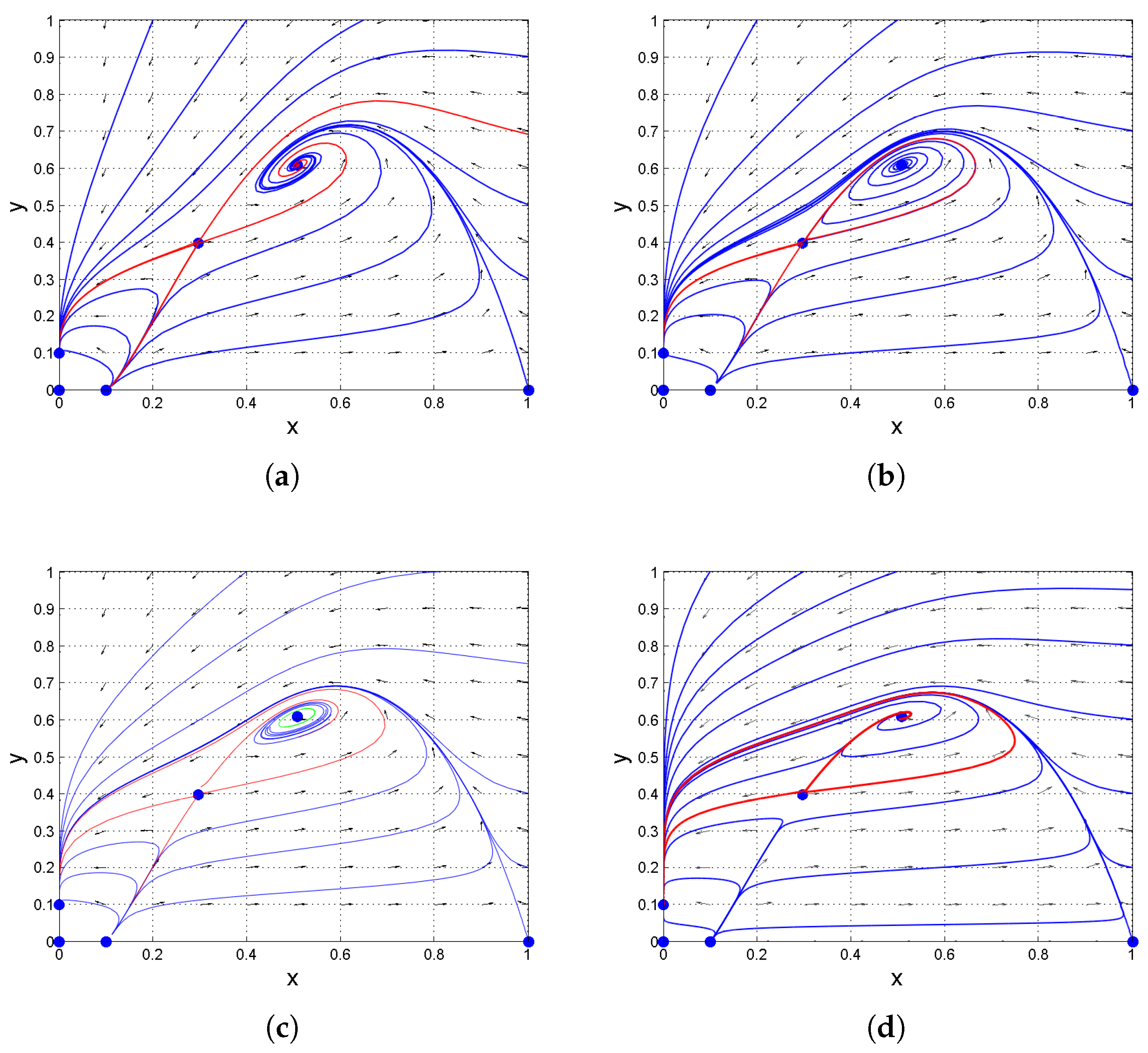
| (saddle) | = (stable), = (saddle) | Figure 2a | |
| (stable) | Homoclinic loop enclosing = (stable), = (saddle) | Figure 2b | |
| (unstable) | Unstable limit cycle (as ) around = (stable), = (saddle) | Figure 2c | |
| (saddle) | = (unstable), = (saddle) | Figure 2d | |
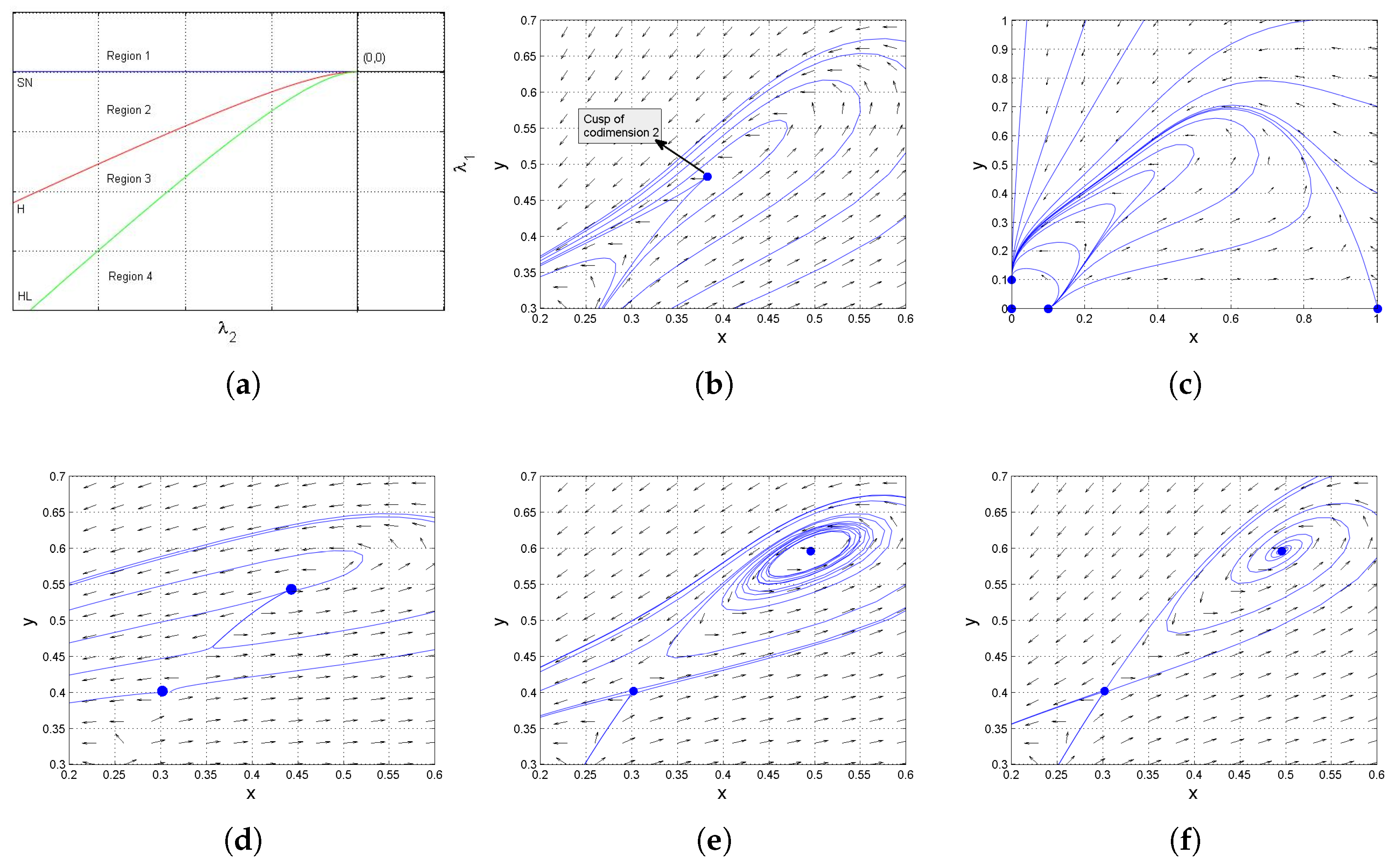
| Region | Number of Interior Equilibrium Points | Dynamic Behavior Exhibited by Regions | Figure |
|---|---|---|---|
| Origin | One | Cusp | Figure 3b |
| Region 1 | Zero | Figure 3c | |
| Region 2 | Two | One was consistently a saddle while the other was unstable | Figure 3d |
| Region 3 | Two | One was consistently a saddle while the other was enclosed by an unstable limit cycle | Figure 3e |
| Region 4 | Two | One was consistently a saddle while the other was stable | Figure 3f |
Disclaimer/Publisher’s Note: The statements, opinions and data contained in all publications are solely those of the individual author(s) and contributor(s) and not of MDPI and/or the editor(s). MDPI and/or the editor(s) disclaim responsibility for any injury to people or property resulting from any ideas, methods, instructions or products referred to in the content. |
© 2024 by the authors. Licensee MDPI, Basel, Switzerland. This article is an open access article distributed under the terms and conditions of the Creative Commons Attribution (CC BY) license (https://creativecommons.org/licenses/by/4.0/).
Share and Cite
Singh, M.K.; Sharma, A.; Sánchez-Ruiz, L.M. Dynamical Complexity of Modified Leslie–Gower Predator–Prey Model Incorporating Double Allee Effect and Fear Effect. Symmetry 2024, 16, 1552. https://doi.org/10.3390/sym16111552
Singh MK, Sharma A, Sánchez-Ruiz LM. Dynamical Complexity of Modified Leslie–Gower Predator–Prey Model Incorporating Double Allee Effect and Fear Effect. Symmetry. 2024; 16(11):1552. https://doi.org/10.3390/sym16111552
Chicago/Turabian StyleSingh, Manoj Kumar, Arushi Sharma, and Luis M. Sánchez-Ruiz. 2024. "Dynamical Complexity of Modified Leslie–Gower Predator–Prey Model Incorporating Double Allee Effect and Fear Effect" Symmetry 16, no. 11: 1552. https://doi.org/10.3390/sym16111552
APA StyleSingh, M. K., Sharma, A., & Sánchez-Ruiz, L. M. (2024). Dynamical Complexity of Modified Leslie–Gower Predator–Prey Model Incorporating Double Allee Effect and Fear Effect. Symmetry, 16(11), 1552. https://doi.org/10.3390/sym16111552