Article

Information Theory in a Darwinian Evolution Population Dynamics Model

Department of Mathematics, Trinity University, 1 Trinity Place, San Antonio, TX 78212, USA
Symmetry 2024, 16(11), 1522; https://doi.org/10.3390/sym16111522
Submission received: 14 October 2024 / Revised: 1 November 2024 / Accepted: 11 November 2024 / Published: 13 November 2024
(This article belongs to the Section Mathematics)

Abstract

:
Since Darwin, evolutionary population dynamics has captivated scientists and has applications beyond biology, such as in game theory where economists use it to explore evolution in new ways. This approach has renewed interest in dynamic evolutionary systems. In this paper, we propose an information-theoretic method to estimate trait parameters in a Darwinian model for species with single or multiple traits. Using Fisher information, we assess estimation errors and demonstrate the method through simulations.

1. Introduction

Evolution can be seen as the dynamic changes in organisms’ traits, driven largely by environmental factors and occurring through mutations or random genetic variations. Darwin’s theory of natural selection ([1]) suggests that species best adapted to their environment pass beneficial traits to their offspring. Over time, advantageous traits may lead to the emergence of new species, making the tracking of trait variations central to understanding evolution.
Information theory offers tools to track such evolutionary changes. For a random variable X depending on a trait parameter θ , the Fisher’s information I ( θ ) measures the information X provides about θ ([2]). Since its introduction ([3]), the Fisher’s information has been widely applied, including in Bayesian statistics ([4]), to derive the Wald’s test ([5]), to estimate Cramér–Rao bounds ([6,7]), in optimal experimental design ([8]), in machine learning ([9]), and in epidemiology ([10]), just to name some. Notably, it connects to relative entropy (or Kullback–Leibler divergence), as the Fisher’s information represents the Hessian of relative entropy with respect to θ . In evolutionary biology, information in genomes is expected to change as environments evolve.
Our focus on evolutionary population dynamics and Fisher information builds on the work of [11], where Darwinian dynamics are explored through evolutionary game theory. They analyze a static game with n players, each choosing a strategy θ i to maximize their payoff f i ( Θ ) , defined by
f i ( Θ ) , i { 1 , 2 , , n } ,
where Θ = ( θ 1 , θ 2 , , θ n ) . This evolves into a dynamic game represented by an ordinary differential equation
x ˙ i = F i ( x , Θ ) , i { 1 , 2 , , n } ,
where x = ( x 1 , x 2 , , x n ) , and F i is the instantaneous payoff for player i. In ecology, this approach adapts to n species, with f i ( Θ ) as the per capita growth rate of a species with density x i and trait θ i . Ref. [12] introduced the G-function to generalize the growth rate:
G ( x , θ , Θ ) | θ = θ i = f i ( x , Θ ) , i { 1 , 2 , , n } ,
where θ is a “virtual variable”. This leads to an evolution equation for strategies:
θ ˙ i = σ 2 g ( x , θ , Θ ) | θ = θ i , where g ( x , θ , Θ ) = ln ( G ( x , θ , Θ ) ) θ .
The connection between game theory and evolution population dynamics can be made using the Table 1 below:
In light of this comparison, estimation of parameters θ i ’s, either in a game theory context or in a population dynamics context, is of paramount importance if one aims to make meaningful predictions, given data, on the underlying model. Now, consider the following population dynamics system:
x ˙ i = x i G ( x , θ , Θ ) | θ = θ i θ ˙ i = σ 2 g ( x , θ , Θ ) | θ = θ i ,
where σ 2 represents the variance of trait distribution. Solutions to this system, called Evolutionarily Stable Strategies (ESSs), provide insight into stable trait configurations ([13,14]). For an ESS, G must attain a maximum at zero with respect to θ ([12]). Recent work on discrete versions of these models includes studies of evolutionary stability ([15]), difference equation schemes ([16]), and applications to disease resistance ([17]). This paper addresses two questions raised in [11]: 1. Are there interpretable relations between the maximum of G, g, and g θ < 0 ? 2. Are there similar interpretable relations for g = 0 and g θ > 0 ?
Our literature review found no comprehensive answers to these questions. To explore them, we frame G in the context of random variables. For one species, if G = G ( x , θ ) represents a density function for a random variable X depending on an unknown trait θ , Fisher information quantifies the information a sample of X contains about θ . By analyzing G and its derivatives, we gain insights into evolutionary traits and parameter estimation. This paper develops a statistical framework for estimating species traits in Darwinian models. By minimizing or maximizing the Fisher’s information in this context, we not only address the questions above but also offer a method for estimating unknown parameters in evolution models. This paper is organized as follows: Section 2 provides an overview of Fisher information in statistics. Section 3 discusses Fisher information within discrete evolutionary population dynamics. Section 4 concludes with final remarks.

2. Review of Fisher’s Information Theory

Let p ( x , θ ) represent the probability density function (pdf) of a random variable X, which can be continuous or discrete on an open set X × Ω R × R n . Here, θ = ( θ 1 , θ 2 , , θ n ) denotes a single parameter or a vector of parameters. Since p ( x , θ ) is a pdf, it must satisfy X p ( x , θ ) d x = 1 . If we have a nonnegative integrable function p 0 ( x , θ ) defined on X , it can be normalized to become a pdf by defining p ( x , θ ) = c p 0 ( x , θ ) , where c = X p 0 ( x , θ ) d x 1 . In what follows, we assume the following conditions on p ( x , θ ) :
(1)
Support independence: The support { x X : p ( x , θ ) 0 } of p is independent of θ .
(2)
Nonnegativity and integrability: p ( · , θ ) is nonnegative for all θ Ω and p L 1 ( X ) .
(3)
Smoothness: p ( x , · ) C 2 ( Ω ) , meaning p ( x , θ ) is continuously differentiable up to the second order with respect to θ for all x R .
The first condition excludes cases like a uniform distribution p ( x , θ ) = 1 θ , where the support varies with θ . The second condition ensures that the log-density f 0 ( x , θ ) = ln ( p ( x , θ ) ) , its first derivative (score function) f 1 ( x , θ ) = θ f 0 ( x , θ ) , and its second derivative f 2 ( x , θ ) = θ 2 f 0 ( x , θ ) are well defined. We denote the expectation of a random variable X by E [ X ] .
Definition 1
(Fisher information). For a random variable X with density p ( x , θ ) satisfying assumptions (1) and (2), the Fisher information of X is defined as
I ( θ ) = E X [ ( f 1 ( X , θ ) ) 2 ] = E X [ f 2 ( X , θ ) ] .
If θ is a vector, then I ( θ ) is a symmetric positive definite matrix, given by
I k l ( θ ) = E X 2 f 0 ( X , θ ) θ k θ l , for 1 k , l n .
The Fisher information I ( θ ) quantifies the amount of information about θ provided by an estimator based on X. When θ is estimated from a random sample X 1 , X 2 , , X n drawn from p ( x , θ ) , the Fisher information in the sample is
I n ( θ ) = n I ( θ ) .
Definition 2
(estimator and properties). Let X be a random variable depending on the parameter vector θ, and let X 1 , X 2 , , X n be a random sample from X. We define the following:
  • Estimator: T = T ( X 1 , X 2 , , X n ) is called an estimator of θ.
  • Unbiased estimator: T is unbiased if E [ T ] = θ .
  • Efficient estimator: An unbiased estimator T is efficient if its variance satisfies Var ( T ) = 1 I n ( θ ) .
In particular, if T = T ( Θ ) is an estimator of Θ based on a sample X 1 , X 2 , , X n , the Cramér–Rao (see for instance [6,7]) bound gives an estimate of the best lower bound for the variance of T as
Var ( T ) ( Θ E ( T ) ) T I n ( Θ ) 1 ( Θ E ( T ) ) .
Equality is obtained in (1) if T is efficient. If T is unbiased, then E [ T ] = Θ and consequently, Θ E [ T ] = 1 , where 1 is a vector of ones R n . Therefore, (1) becomes
Var ( T ) = I n ( Θ ) 1 .
Example 1.
Suppose X is a random variable with distribution f ( x , θ ) = θ e θ x , where θ > 0 . Then we have that λ ( x , θ ) = ln ( θ ) θ x , g ( x , θ ) = 1 θ x , and h ( x , θ ) = 1 θ 2 . It follows that I ( θ ) = E X [ h ( x , θ ) ] = 1 θ 2 and I n ( θ ) = n θ 2 . If we now consider a random sample X 1 , X 2 , , X n from X, and T = T ( θ ) = 1 n i = 1 n X i , we note that E [ X i ] = θ , so that E [ T ] = θ . Thus, T is an unbiased estimator of θ and d d θ T = 1 . Moreover, V a r ( T ) = θ 2 n . We then verify from (2) that indeed we have V a r ( T ) = θ 2 n = 1 I n ( θ ) . Consequently, accurate estimates of Θ have large Fisher’s information (matrix) components, whereas inaccurate ones have small Fisher’s information components.

3. Evolution Population Dynamics and Information Theory

3.1. Single Population Model with One Trait

Consider the following discrete evolutionary dynamical model:
x t + 1 = x t G ( x t , θ t , u t ) θ t + 1 = θ t + σ 2 g ( x t , θ t , u t ) ,
where G ( x , θ , u ) = b ( θ ) e c u ( θ ) x where b ( θ ) = b 0 e θ 2 2 w 2 and c u ( θ ) = c 0 e κ ( θ u ) , for a constant u and for some positive constants σ (speed of evolution), b 0 (initial birth rate), c 0 (competition constant), κ , and w (standard deviation of the distribution of birth rates), and for a differentiable function c u ( θ ) of θ and positive and continuous function b ( θ ) . This system has nontrivial fixed points ( x * , θ * ) if they satisfy the equations
1 = b ( θ ) e c u ( θ ) x 1 b ( θ ) = c u ( θ ) x .
This can further be reduced to the condition on b ( θ ) and c u ( θ ) given by
ln ( b ( θ ) ) c u ( θ ) = 1 b ( θ ) c u ( θ ) .
The theorem below shows how to obtain the Fisher’s information of the above system as a function of the system’s parameters.
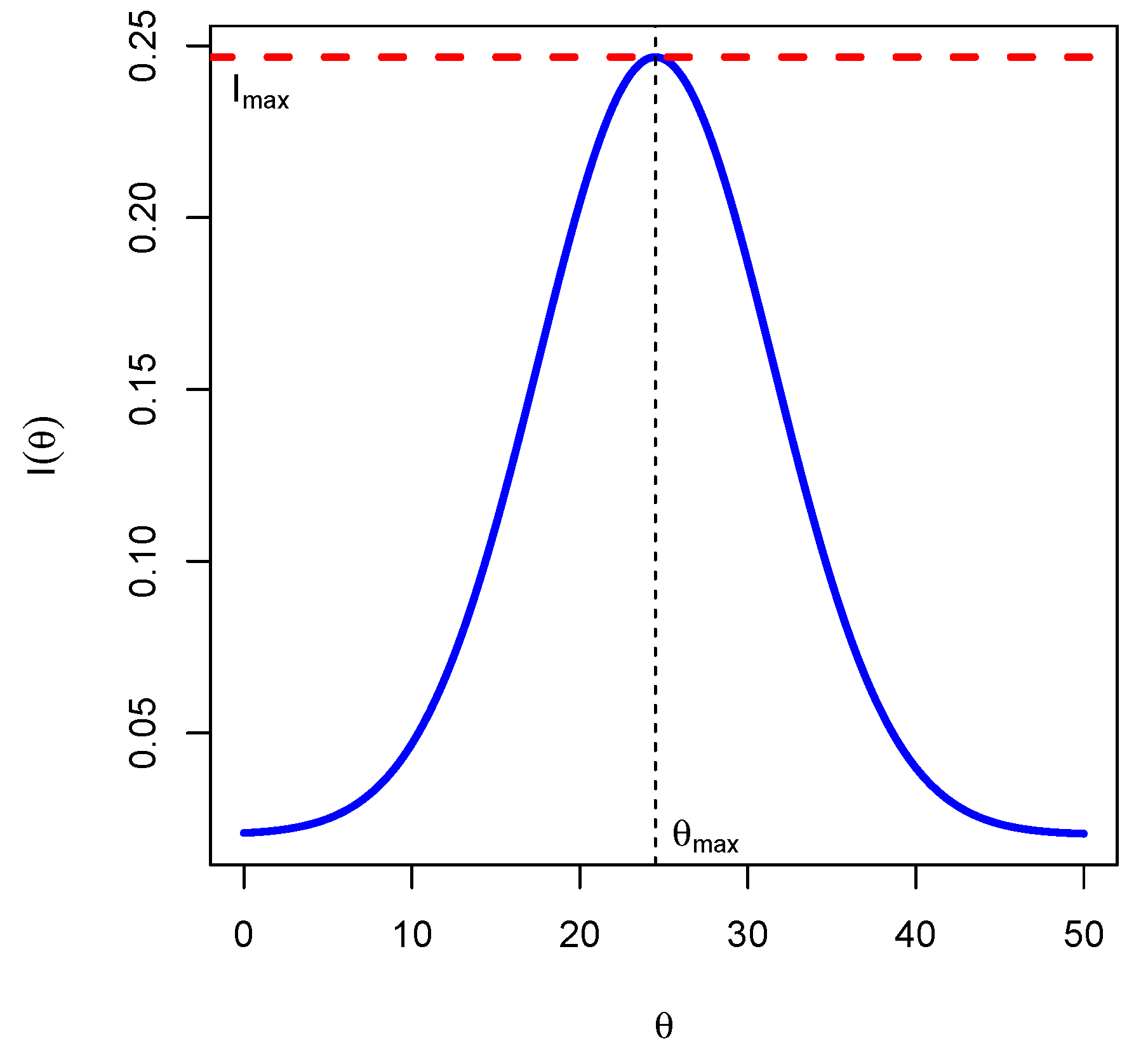
Theorem 1.
Let Γ u ( θ ) = b ( θ ) c u ( θ ) . Then the Fisher’s information of this system is constant and given by
I ( θ ) = 1 ω 2 + κ 2 Γ u ( θ ) .
The proof can be found in Appendix A.1.
  • The corollary below shows that the Fisher’s information has a maximum value, see Figure 1 below for an illustration.
Corollary 1.
The Fisher’s information I ( θ ) attains its maximum value I m a x for θ m a x = w 2 κ , and the maximum value is
I m a x = 1 w 2 + κ 2 b 0 c 0 e 1 2 ( w κ ) 2 κ u .
The proof can be found in Appendix A.2.
In the proposition below, we give precise conditions for the existence of nontrivial fixed points of the system above.
Proposition 1.
Let
ξ 1 = 1 κ 2 + 2 w 2 ln ( b 0 ) .
If ξ 1 < 0 , then the Darwinian system (9) does not have a nontrivial critical point.
If ξ 1 = 0 , then the Darwinian system has a unique nontrivial fixed point ( x * , θ * ) given as
x * = ln ( b 0 ) θ * 2 w 2 c 0 e κ ( θ * u ) , θ * = 1 κ .
If ξ 1 > 0 , then the Darwinian system has two nontrivial fixed points ( x + , θ + ) and ( x , θ ) given by
x ± = ln ( b 0 ) θ ± 2 w 2 c 0 e κ ( θ ± u ) , θ ± = 1 κ ± ξ 0 .
Proposition 1 and Theorem 1 are important in that when θ t θ as t , then by continuity of the function I ( θ ) with respect to θ , we will have I ( θ t ) I ( θ ) as t . This means that the Fisher’s information, over time, will be maximized at the critical point ( x , θ ) of the dynamical system. Therefore, for estimation purposes, the reciprocal of I ( θ ) will be the smallest variance for any unbiased estimator of the trait θ . In Figure 2, below, we use the following parameters: w = 3 ; κ = 3 ; b 0 = 10 ; c 0 = 0.5 ; u = 1 ; σ = 5 ; n = 750 ; x 0 = 1 ; θ 0 = 10 .
  • Special case:
We will now discuss the particular case of an exponential distribution, that is, b ( θ ) = c u ( θ ) = θ . Clearly, the condition (5) is satisfied with θ = θ * = : e and x = x * : = e 1 . Therefore,
G ( x , θ ) = θ e θ x , λ ( x , θ ) = ln ( θ ) θ x , g ( x , θ ) = 1 θ x , h ( x , θ ) = 1 θ 2 .
This implies that I ( θ ) = E X [ h ( X , θ ) ] = 1 θ 2 . It follows that there are equilibrium fixed points: the extinction equilibrium (trivial point) E 0 = ( 0 , 0 ) and the interior equilibrium (nontrivial point)
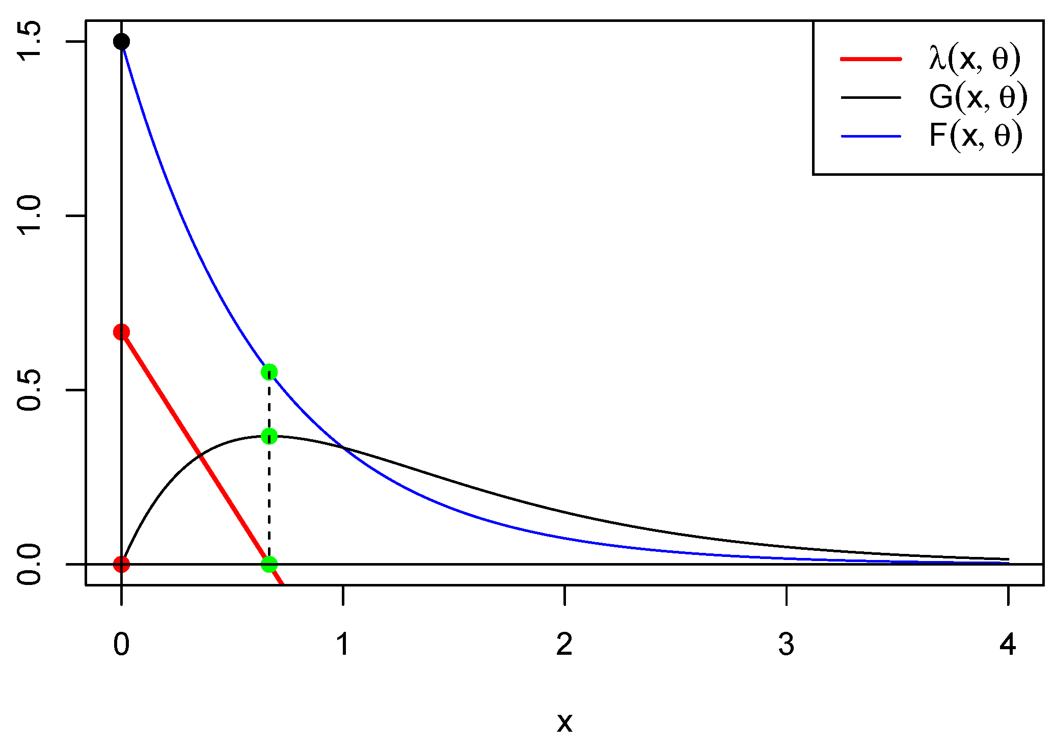
 E 1 = ( e 1 , e ) . In Figure 3, below, we represent functions G ( x , θ ) , F ( x , θ = x G ( x , θ ) , and λ ( x , θ ) for θ = 3 2 . This shows that λ ( x , θ ) is minimized where G ( x , θ ) is maximized, providing a clue as to the relation between the maximum of G and the critical points of g and g θ . Another clue can be found in Figure 4 below.
From a dynamical systems’ perspective, it means that X t , the value of X at time t, is generated from the distribution G ( x , θ ) and used to calculate the value of X t + 1 . Therefore, the role of the first choice of θ is to initialize the dynamical system. Once the system is initialized for X t , we can use an information theory approach to provide an estimator T ( θ ) of θ t , the value of θ at time t. That estimator, if efficient, will have variance I n ( θ t ) 1 . We can then use the dynamical system (9) to estimate θ t + 1 , and the Fisher’s information will provide its variance. We note that θ t + 1 will only be an estimate of the true value and therefore will carry an error as t changes. It is therefore expected that at the nontrivial critical point (ESS) ( x * , θ * ) of the dynamical system, the estimator T ( θ ) converges to θ * and the variance of T ( θ ) converges to I n ( θ * ) 1 as t .
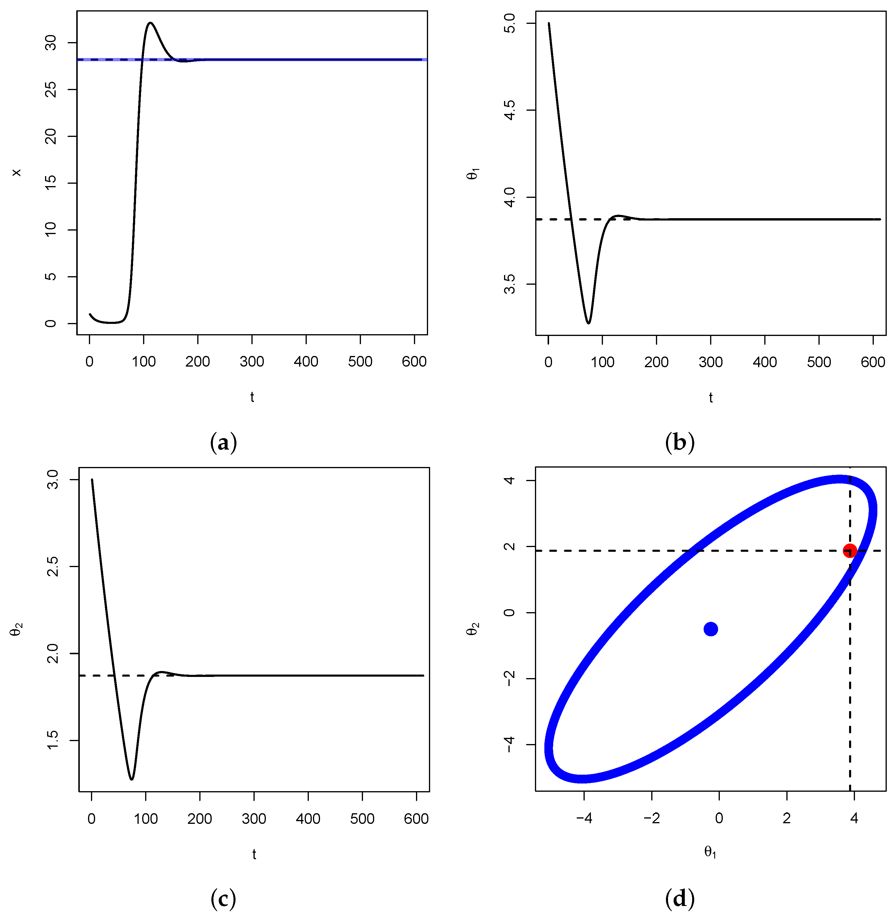
Figure 5 below is an illustration of this fact for G ( x , θ ) = θ e θ x .
Indeed, we generated two random samples of size n = 50 (Figure 5a,b) and n = 250 (Figure 5c,d) with t = 1 , 2 , m where m = 10 and σ = 0.04 from exponential distributions with respective initial parameters θ 0 = 0.2 , 2.13 . We choose T n ( θ t ) = 1 n i = 1 n X i , which is known to be an efficient estimator of θ . The dashed lines represent the respective values of T n ( θ t ) , and the black lines represent their 95% confidence intervals ( T n ( θ t ) 1.96 I n ( θ t ) 1 , T n ( θ t ) + 1.96 I n ( θ t ) 1 ) . This shows in particular that on average, T n ( θ t ) converges to e (dashed line), the fixed point of the dynamical system, as expected from the above. It also shows that as the Fisher’s formation gets larger, the variance of the estimator gets smaller and thus the width of the confidence interval gets smaller and quickly approaches zero as in Figure 5c,d. The conclusion is that given an evolution dynamical system, we can estimate the evolution parameter vector Θ and provide an estimate of the error on the estimate that is the inverse of the Fisher’s information. Moreover, over time, the estimate converges to the ESS of the system (when it exists) and the errors on the estimate essentially becomes zero when convergence is reached.
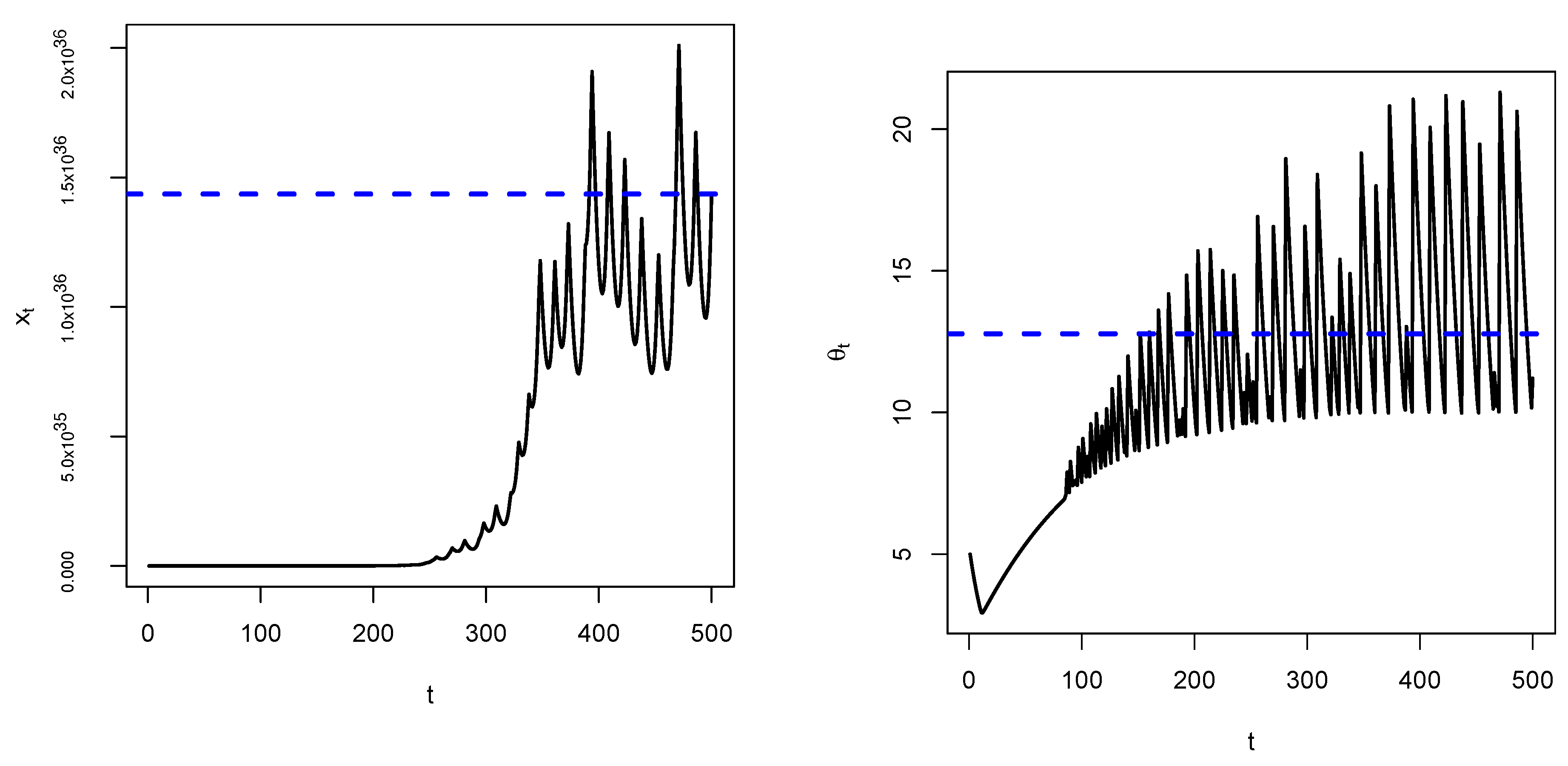
Remark 1.
We observe that convergence of θ t towards e as predicted depends on choosing an appropriate value of σ. Large values of σ will definitely make the system unstable as oscillations will slowly and increasingly occur, see Figure 6 below.

3.2. Discussion

Assumption A 1 is important in that we only require that G be nonnegative and G L 1 ( Ω ) , which guarantees that it can be transformed into the density of a random variable. It does not, however, guarantee that we can easily obtain a sample from it! If G happens to be a classical distribution (normal, exponential, t-distribution, Weibull, etc.), then there are sampling methods already available. If G has a nonclassic expression, we may have to resort to either the Probability Integral Transform (see Theorem 2.1.10, p. 54 in [18]) or to Markov Chain Monte Carlo (MCMC) to obtain a sample, which sometimes are themselves onerous in terms of time. Obtaining an efficient estimator of θ is easily undertaken when G is a classic distribution. While efficiency would be great, it may not be necessary since over time, the estimator would still converge, albeit slowly, to the fixed point of θ . We observe that the estimates we obtain in this case are point estimates of T n ( θ t ) (mean, median, etc.), albeit at each time t. A Bayesian estimate is also possible, provided that the initial distribution of θ 0 is selected from a well-defined Jeffrey’s prior. As for answers to the questions raised in the Introduction, we can say based on the above that the set of points ( x , θ ) where G ( x , θ ) is maximized is the same where ln ( G ( x , θ ) ) is minimized and contains all the critical points of the function G. This can be written formally as Arg max θ Ω G ( x , θ ) = Arg min θ Ω ln ( G ( x , θ ) ) ( x , θ ) X × Ω : g ( x , θ ) = 0 .

3.3. Single Population Model with Multiple Traits

Now suppose we are in the presence of one species with density x possessing n traits given by the vector Θ = ( θ 1 , θ 2 , , θ n ) and a vector U = ( u 1 , u 2 , , u n ) .
( H 1 ) We assume that b ( Θ ) = b 0 e x p i = 1 n θ i 2 2 w i 2 is the joint distribution of the independent traits θ i , each with mean 0 and variance w i 2 .
( H 2 ) We also assume that c U ( Θ ) = c 0 e x p i = 1 n κ i ( θ i u i ) .
( H 3 ) We assume that the density of x t is given as G ( x , Θ , U ) = b ( Θ ) exp ( c U ( Θ ) x ) at t = 1 .
Under H 1 , H 2 , and H 3 , we consider the discrete dynamical system
x t + 1 = x t G ( x t , Θ t , U t ) Θ t + 1 = Θ t + Σ g ( x t , Θ t , U t ) ,
where
Σ = σ 11 σ 12 σ 1 n σ 21 σ 22 σ 2 n σ n 1 σ n 2 σ n n .
Remark 2.
There are a couple of distinctions between this model and the ones encountered in the recent literature, see for instance [16,19]. Firstly, the matrix Σ considered here is not necessarily symmetric ( σ i j σ j i ). Secondly, the competition function c U ( Θ ) depends subtly on a vector U that need not be the mean of Θ, as it is often considered. We note, however, that when Θ = U , then c U ( Θ ) = c 0 . Ecologically, this happens when competition is maximal. This leads to recovering the uncoupled Darwinian model (2) in [19].
The result below shows how to obtain the Fisher’s information of the Darwinian dynamical system (9).
Theorem 2.
Let Γ U ( Θ ) = b ( Θ ) c U ( Θ ) . Then under assumptions H 1 , H 2 , and H 3 , the dynamical system above has the Fisher’s information matrix I ( Θ ) given as
I ( Θ ) = 1 w 1 2 + κ 1 2 Γ U ( Θ ) κ 1 κ 2 Γ U ( Θ ) κ 1 κ n Γ U ( Θ ) κ 1 κ 2 Γ U ( Θ ) 1 w 2 2 + κ 2 2 Γ U ( Θ ) κ 2 κ n Γ U ( Θ ) κ 1 κ n Γ U ( Θ ) κ 2 κ n Γ U ( Θ ) 1 w n 2 + κ n 2 Γ U ( Θ ) .
The proof of this result can be found in Appendix B.
Remark 3.
We observe that in the case of a high-dimension vector of parameters Θ, the theorem above gives us not only the variance (the diagonal terms of I ( Θ ) ) on the estimator of each component of Θ but also the covariances between pairs of estimates (the off-diagonal terms) of different components (or traits). This may be important, especially to distinguish correlated and noncorrelated traits or strategies.
A necessary condition for the existence of an extinction equilibrium ( 0 , 0 ) for this system is that det ( Σ ) 0 . Letting ρ ( A ) represent the spectral radius of matrix A, it was proved in [16] that if ρ ( I + Σ h ( 0 , 0 ) ) < 1 and b 0 < 1 , then the extinction equilibrium is asymptotically stable and unstable if ρ ( I + Σ h ( 0 , 0 ) ) < 1 and b 0 > 1 , or if ρ ( I + Σ h ( 0 , 0 ) ) > 1 for all b 0 > 0 . This is particularly true if Σ is diagonally dominant and for σ 12 = σ 21 = 0 . This system admits a nontrivial fixed point (positive equilibrium) ( x * , Θ * ) if G ( x * , Θ * ) = 1 and det ( Σ ) = 0 . In the proposition below, we give a more precise characterization of nontrivial fixed points of the system (15).
Proposition 2.
Assume d e t ( Σ ) = 0 and σ i i 0 for i , j = 1 , , n . Put
μ i j = σ i j σ i i , ν j = κ j + i = 1 , i j n μ i j κ i ,
and given j 1 , 2 , , n
ξ n j : = 1 ν j 2 1 w j 2 + i = 1 , i j n μ i j 2 w i 2 + 2 ln ( b 0 ) .
If ξ n j < 0 , then there is no nontrivial solution for the system (9).
Now suppose ξ n j 0 . Then the system (9) has a nontrivial solution ( x * , Θ * ) given as
x = ln ( b 0 ) i = 1 n ( θ i ) 2 2 w i 2 c 0 e x p i = 1 n κ i ( θ i u i ) ,
and
(i) 
If ξ n j = 0 , then Θ = 1 ν , μ 2 ν , , μ n ν .
(ii) 
If ξ n j > 0 , then the coordinates of the vector Θ * are points that lie on the curve of equation
1 w j 2 θ j + 1 ν 2 + i = 1 , i j n 1 w i 2 θ i + μ i j ν j 2 ξ n j = 0 .
The proof can be found in Appendix C.
  • Special case: single species with two traits.
Here we consider the particular case of a system of one species with two traits, namely, the coupled dynamical system
x t + 1 = x t G ( x t , θ 1 , t , θ 2 , t ) θ 1 , t + 1 = θ 1 , t + σ 11 g 1 ( x t , θ 1 , t , θ 2 , t ) + σ 12 g 2 ( x t , θ 1 , t , θ 2 , t ) θ 2 , t + 1 = θ 2 , t + σ 21 g 1 ( x t , θ 1 , t , θ 2 , t ) + σ 22 g 2 ( x t , θ 1 , t , θ 2 , t ) .
The fixed points ( x , θ 1 , θ 2 ) of this model are solutions of the system of equations
x G ( x , u , v ) = x Σ g ( x , u , v ) = 0 ,
where
Σ = σ 11 σ 12 σ 21 σ 22 , for ( u , v ) R 2 .
Corollary 2.
Assume σ 11 , σ 22 0 and σ 11 σ 22 = σ 12 σ 21 . We put
μ 1 = σ 21 σ 22 , μ 2 = σ 12 σ 11 , ν = κ 1 + μ 2 κ 2 ,
and
ξ 2 : = 1 ν 2 1 w 1 2 + μ 2 2 w 2 2 + 2 ln ( b 0 ) .
If ξ 2 < 0 , then there is no nontrivial solution for the system (14).
Now suppose ξ 2 0 . Then the system (14) has a nontrivial solution ( x , θ 1 , θ 2 ) given as
x = ln ( b 0 ) i = 1 n ( θ i ) 2 2 w i 2 c 0 e x p i = 1 n κ i ( θ i u i ) , f o r   n = 2 .
and
(i) 
If ξ 2 = 0 , then ( θ 1 , θ 2 ) = 1 ν , μ 2 ν .
(ii) 
If ξ 2 > 0 , then ( θ 1 , θ 2 ) are points that lie on the ellipse of equation
θ 1 + 1 ν 2 a 2 + θ 2 + μ 2 ν 2 b 2 = 1 , w h e r e   a = w 1 ξ 2   a n d   b = w 2 ξ 2 .
In Figure 7, below, we illustrate Proposition 2 for x 0 = 1 , θ 10 = 3 ; θ 20 = 5 ; w 1 = 4 ; w 2 = 1 ; κ 1 = 3 ; κ 2 = 0.5 , σ 11 = 0.1 ; σ 21 = 1 ; σ 11 = 1 ; σ 12 = 2 ; σ 22 = 2 ; u 1 = 3 ; u 2 = 0 , c 0 = 0.1 . We verify that μ 1 = σ 21 / σ 22 = 0.5 and μ 2 = σ 12 / σ 11 = 2 . Therefore, μ 1 μ 2 = 1 , that is, det ( Σ ) = 0 . We also have that ν = 4 and that ξ 2 4.86 > 0 . Hence, according to Proposition 2 above, ( θ 1 , θ 2 ) is expected to be on the ellipse centered as ( 1 / ν , μ 2 / μ ) = ( 0.25 , 0.5 ) with respective major and minor axis lengths a = w 1 ξ 8.82 and b = w 2 ξ 2.21 .
The parameters for Figure 8 are the same except for θ 10 = 3 , θ 20 = 1 and x 0 is generated from an exponential distribution with parameters c U ( Θ ) = c 0 exp i = 1 n κ i ( θ i 0 u i ) .

3.4. Discussion

An important remark about Theorem 2 is that we assume the vector U is given. In fact, if the vector Θ were given, the same technique could have been used for the estimation of U, up to a negative sign on the Fisher’s information matrix. Having U be different from the average of Θ allows for generalization, in that Θ U represents the difference of a set of traits Θ from a given set of traits U, which need not be the average of Θ . One thing we have not insisted much about in this paper is the type of estimator of Θ itself. We do not need to specify in particular which estimator to use, since the inverse of the Fisher’s information is the smallest variance for all estimators. One consequence of Proposition 2 above is that once we have estimated Θ * , we can deduce the value of x * . The results above also show that there may be many equilibria when ξ n > 0 . In the context of evolution and natural selection, one should focus on equilibria that ensure better adaptation to environmental fluctuations. This specifically means adding stochasticity to the model by means of, say, a Wiener process and finding traits that ensure, for example, that on average, the species density is bounded away from the extinction equilibrium. Another possibility could be to focus on equilibria that maximize the species density in order to increase the prospects of survivability of the species. This can be performed using a constraint optimization problem max u R n f ( U ) where f ( U ) = x * subject to the constraint that the point u be on the curve defined in Equation (13). In the particular case where n = 2 with U = ( u , v ) , we have
f ( u , v ) : = ln ( b 0 ) u 2 2 w 1 2 v 2 2 w 2 2 c 0 exp κ 1 ( u u i ) κ 2 ( v u i ) .
However, the form of the function f ( u , v ) makes it a very challenging problem. Rewriting, we have
f ( u , v ) : = c 0 1 ln ( b 0 ) u 2 2 w 1 2 v 2 2 w 2 2 e κ 1 ( u u i ) + κ 2 ( v u i ) .
We observe that for positive κ 1 and κ 2 , the function ( u , v ) e κ 1 ( u u i ) + κ 2 ( v u i ) is a positive and increasing function of u and v. Therefore, maximizing f ( u , v ) amounts to maximizing
f * ( u , v ) = ln ( b 0 ) u 2 2 w 1 2 v 2 2 w 2 2 .
Geometrically, this is the equation of a paraboloid that bends down. Therefore, the constraint optimization amounts to finding the points of intersection between a paraboloid and an ellipse. This means there can be between 0 and 4 points of intersection. Finally, let us observe that the expression of x * in the case of multiple traits is just a generalization of the case of one trait. In fact, the first equation in the system (4) can be written as x * = ln ( b ( θ ) ) c u ( θ ) . We see that this is similar to the expression of x * given in Equation (A3) for two traits, which naturally generalizes to the case of one species with n 2 traits.

4. Conclusions

In this paper, we introduced a method for estimating trait coefficients in a Darwinian evolution population dynamics model by employing the Fisher information matrix. This approach enables us not only to estimate traits effectively but also to characterize the uncertainty inherent in the estimation process. Our study focuses on two specific cases: a single species with one trait and a single species with multiple traits. Extending this framework to scenarios involving multiple species with one or more traits represents an intriguing avenue for future research, offering the potential to understand interspecies interactions in greater detail.
An essential contribution of our work is the proposed relationship between the G-function, its natural logarithm, and its derivative g. This relationship facilitates a more nuanced understanding of evolutionary dynamics and provides a clearer basis for examining trait adaptation over time. As a by-product, our method yields a precise characterization of the nontrivial fixed points of the model. Specifically, we demonstrated that once the critical density x * is determined, the set of critical traits Θ * aligns along a well-defined curve in R n . Conversely, if the set of critical traits Θ * is known, there may exist a unique critical density x * for the Darwinian system. Notably, this density may not necessarily ensure the survival of the species, adding complexity to our understanding of stable evolutionary states.
In addition to the traditional approach, we explored the potential of using modern machine learning techniques for trait parameter estimation. Traits could be estimated by minimizing relative information, such as Kullback–Leibler divergence, within a Darwinian evolution population model. This could be achieved via either classical gradient ascent or stochastic gradient ascent methods, with careful consideration given to selecting appropriate weights for the minimization process. Both approaches would need to be tailored to suit supervised or unsupervised learning environments, depending on the data availability and modeling goals.
Looking ahead, an extension of this work could involve introducing stochasticity into the model, for example, by incorporating a Wiener process. Such a modification would allow us to examine strong persistence on average, study the existence of global solutions, and explore stationary distributions within the population dynamics framework. This stochastic extension would provide a richer understanding of the model’s behavior under real-world conditions, where randomness and environmental variability play a significant role in shaping evolutionary outcomes.

Funding

This research was funded by AMS-Simon Research Enhancement for PUI grant.

Data Availability Statement

The data used in this paper are all simulated.

Conflicts of Interest

The author declares no conflicts of interest. The funders had no role in the design of the study; in the collection, analyses, or interpretation of data; in the writing of the manuscript; or in the decision to publish the results.

Appendix A

Appendix A.1. Proof of Theorem 1

Proof. 
We have that λ ( x , θ ) = ln ( G ( x , θ ) ) = ln ( b 0 ) θ 2 2 w 2 c 0 x e κ ( θ u ) .
It follows that
g ( x , θ ) = θ w 2 + κ c 0 x e κ ( θ u ) = θ w 2 + κ c u ( θ ) x ,
and
h ( x , θ ) = 1 w 2 κ 2 c 0 x e κ ( θ u ) .
From Definition 1 above, it follows that
I ( θ ) = E X [ h ( X , θ ) ] = E X 1 w 2 κ 2 c u ( θ ) X = 1 w 2 + κ 2 c u ( θ ) E [ X ] .
We observe that X has probability distribution G ( x , θ ) = b ( θ ) e c u ( θ ) x ; therefore,
E [ X ] = X x G ( x , θ ) d x = b ( θ ) c u ( θ ) X x c u ( θ ) e c u ( θ ) x d x = b ( θ ) c u ( θ ) 2 .
It then follows that
I ( θ ) = 1 w 2 + κ 2 c u ( θ ) b ( θ ) c u ( θ ) 2 = 1 w 2 + κ 2 b ( θ ) c u ( θ ) = 1 w 2 + κ 2 Γ ( θ ) .
This ends the proof of the Theorem. □

Appendix A.2. Proof of Corollary 1

Suppose b 0 c 0 = 1 κ 2 π w κ e κ u ( w κ ) 2 2 . From Equation (A1) above, we have that
I ( θ ) = 1 w 2 + κ 2 b 0 c 0 e θ 2 2 w 2 + κ ( θ u ) .
Completing the square, we have that
θ 2 2 w 2 + κ ( θ u ) = 1 2 w 2 θ 2 2 w 2 κ θ + 2 w 2 κ u = 1 2 w 2 ( θ w 2 κ ) 2 w 4 κ 2 + 2 w 2 κ u = 1 2 w 2 ( θ w 2 κ ) 2 + 1 2 ( w κ ) 2 κ u .
It follows that
I ( θ ) = 1 w 2 + κ 2 b 0 c 0 e 1 2 ( w κ ) 2 κ u e 1 2 w 2 ( θ w 2 κ ) 2 .
From the given expression of b 0 c 0 above, it follows that that
I ( θ ) = 1 w 2 + 1 w 2 π e 1 2 w 2 ( θ w 2 κ ) 2 .

Appendix B. Proof of Theorem 2

Proof. 
Let b ( Θ ) = b 0 exp i = 1 n θ i 2 2 w i 2 and c U ( Θ ) = c 0 exp i = 1 n κ i ( θ i u i ) .
We have that
G ( x , Θ ) = b 0 exp i = 1 n θ i 2 2 w i 2 c 0 x exp i = 1 n κ i ( θ i u i ) = b ( Θ ) e c U ( Θ ) x ,
from which we can deduce
λ ( x , Θ ) = ln ( b 0 ) i = 1 n θ i 2 2 w i 2 c 0 x exp i = 1 n κ i ( θ i u i ) = ln ( b ( Θ ) ) x c U ( Θ ) .
It follows that g ( x , Θ ) is the vector given as
g ( x , Θ ) : = ( g i ( x , Θ ) ) i = 1 , , n : = θ i w i 2 + c 0 κ i x exp i = 1 n κ i ( θ i u i ) i = 1 , 2 , , n .
Hence, h ( x , Θ ) is an n × n matrix given by
h ( x , Θ ) = g 11 ( x , Θ ) g 12 ( x , Θ ) g 1 n ( x , Θ ) g 21 x , Θ ) g 22 ( x , Θ ) g 2 n ( x , Θ ) g n 1 ( x , Θ ) g n 2 ( x , Θ ) g n n ( x , Θ ) ,
where for i = 1 , 2 , , n , we have
g i i ( x , Θ ) = 2 λ θ i 2 = 1 w i 2 c 0 κ i 2 x exp i = 1 n κ i ( θ i u i ) = 1 w i 2 κ i 2 c U ( Θ ) x .
and
g i j ( x , Θ ) = 2 λ θ i θ j = c 0 κ i κ j x exp i = 1 n κ i ( θ i u i ) = κ i κ j c U ( Θ ) x .
We can deduce that I ( Θ ) is the n × n matrix given as
I 11 ( Θ ) I 12 ( Θ ) I 1 n ( Θ ) I 21 x , Θ ) I 22 ( Θ ) I 2 n ( Θ ) I n 1 ( Θ ) I n 2 ( Θ ) I n n ( Θ ) ,
where
I i i ( Θ ) = E X 2 λ ( X , Θ ) θ i 2 = 1 w i 2 + κ i 2 c U ( Θ ) E [ X ] .
Since X has distribution G ( x , Θ ) , we have that
E [ X ] = X x G ( x , Θ ) d x = b ( Θ ) c U ( Θ ) X x c U ( Θ ) e c U ( Θ ) x d x = b ( Θ ) c U ( Θ ) · 1 c U ( Θ ) .
Therefore, we have that
I i i ( Θ ) = 1 w i 2 + κ i 2 b ( Θ ) c U ( Θ ) = 1 w i 2 + κ i 2 Γ U ( Θ ) .
Likewise, for i j ,
I i j = E X 2 λ ( X , Θ ) θ i θ j = κ i κ j c u ( θ ) E [ X ] = κ i κ i b ( Θ ) c U ( Θ ) = κ i κ i Γ U ( Θ ) .

Appendix C. Proof of Proposition 2 and Corollary 2

Proof. 
The proof of Proposition 2 is an easy generalization from the two-traits model.
First, assume that we are in the presence of two traits.
We have that
det ( Σ ) = 0 σ 11 σ 22 = σ 12 σ 21 μ 1 μ 2 = 1 .
The system in (14) has a non-trivial solution if Σ g ( x , Θ ) = 0 , that is,
g 1 ( x , θ 1 , θ 2 ) + μ 2 g 2 ( x , θ 1 , θ 2 ) = 0 μ 1 g 1 ( x , θ 1 , θ 2 ) + g 2 ( x , θ 1 , θ 2 ) = 0 .
We will show in the sequel that either of the Equations in (A2) can be used to characterize the solutions ( θ 1 , θ 2 ) . Let H = c 0 exp i = 1 n κ i ( θ i u i ) for n = 2 . From the first Equation in (15), we have
G ( x , θ 1 , θ 2 ) = 1 b 0 exp i = 1 n θ i 2 2 w i 2 c 0 x exp i = 1 n κ i ( θ i u i ) = 1 b 0 = exp i = 1 n θ i 2 2 w i 2 + c 0 x exp i = 1 n κ i ( θ i u i ) b 0 = exp i = 1 n θ i 2 2 w i 2 + x H ln ( b 0 ) = i = 1 n θ i 2 2 w i 2 + x H .
It therefore follows that
x = ln ( b 0 ) i = 1 n θ i 2 2 w i 2 H .
Next, we define
ξ 2 = 1 ν 2 1 w 1 2 + μ 2 2 w 2 2 + 2 ln ( b 0 ) .
Therefore, for a solution ( x , θ 1 , θ 2 ) of (15), we have
g 1 ( x , θ 1 , θ 2 ) + μ 2 g 2 ( x , θ 1 , θ 2 ) = θ 1 w 1 2 + x κ 1 H + μ 2 θ 2 w 2 2 + x κ 2 H = θ 1 w 1 2 + μ 2 θ 2 w 2 2 + x H ( κ 1 + μ 2 κ 2 ) = θ 1 w 1 2 + μ 2 θ 2 w 2 2 + ν ln ( b 0 ) θ 1 2 2 w 1 2 θ 2 2 2 w 2 2 = ν 2 w 1 2 θ 1 2 1 w 1 2 θ 1 ν 2 w 2 2 θ 2 2 μ 2 w 2 2 θ 2 + ν ln ( b 0 ) . = ν 2 w 1 2 θ 1 2 + 2 ν θ 1 ν 2 w 2 2 θ 2 2 + 2 μ 2 ν θ 2 + ν ln ( b 0 ) . = ν 2 w 1 2 θ 1 + 1 ν 2 + ν 2 w 1 2 1 ν 2 ν 2 w 2 2 θ 2 + μ 2 ν 2 + ν 2 w 2 2 μ 2 2 ν 2 + ν ln ( b 0 ) . = ν 2 w 1 2 θ 1 + 1 ν 2 ν 2 w 2 2 θ 2 + μ 2 ν 2 + 1 2 w 1 2 ν + μ 2 2 2 w 2 2 ν + ν ln ( b 0 ) .
Dividing the latter by ν 2 , we have that
g 1 ( x , θ 1 , θ 2 ) + μ 2 g 2 ( x , θ 1 , θ 2 ) = 0 1 w 1 2 θ 1 + 1 ν 2 1 w 2 2 θ 2 + μ 2 ν 2 + 1 w 1 2 ν 2 + μ 2 2 w 2 2 ν 2 + 2 ln ( b 0 ) = 0 . 1 w 1 2 θ 1 + 1 ν 2 1 w 2 2 θ 2 + μ 2 ν 2 ξ 2 = 0
Clearly, if ξ 2 < 0 , there is no solution to g 1 ( x , θ 1 , θ 2 ) + μ 2 g 2 ( x , θ 1 , θ 2 ) = 0 .
If ξ 2 = 0 , then
g 1 ( x , θ 1 , θ 2 ) + μ 2 g 2 ( x , θ 1 , θ 2 ) = 0 ( θ 1 , θ 2 ) = 1 ν , μ 2 ν .
If ξ 2 > 0 , we let
a = w 1 ξ 2 , b = w 2 ξ 2 .
It follows that
g 1 ( x , θ 1 , θ 2 ) + μ 2 g 2 ( x , θ 1 , θ 2 ) = 0 θ 1 + 1 ν 2 a 2 + θ 2 + μ 2 ν 2 b 2 = 1 .
That is, the ellipse centered at ( θ 1 0 , θ 2 0 ) = 1 ν , μ 2 ν with respective major and minor axis lengths a and b. Similar to above, we define
ξ * = 1 ν * 2 μ 1 w 1 2 + 1 w 2 2 + 2 ln ( b 0 ) , where   ν * = μ 1 κ 1 + κ 2 .
If ξ * > 0 , then
μ 1 g 1 ( x , θ 1 , θ 2 ) + g 2 ( x , θ 1 , θ 2 ) = 0 θ 1 + μ 1 ν * 2 a * 2 + θ 2 + 1 ν * 2 b * 2 = 1 .
That is, the ellipse centered at ( θ 1 0 , θ 2 0 ) = μ 1 ν , 1 ν with respective major and minor axis lengths
a = w 1 ξ , b = w 2 ξ .
We observe that the two ellipses are the same:
(1)
They have identical centers. Indeed, we have ν = μ 2 ν * and 1 ν = 1 μ 2 ν * = μ 1 ν * since det ( Σ ) = 0 implies that μ 1 μ 2 = 1 . Likewise, we have 1 ν * = μ 2 ν .
This proves that ( θ 1 0 , θ 2 0 ) = ( θ 1 0 , θ 2 0 ) , that is, the two centers are identical.
(2)
They have the same parameters. Indeed, we have
1 ν 2 1 w 1 2 + μ 2 2 w 2 2 = 1 μ 2 2 ν * 2 1 w 1 2 + μ 2 2 w 2 2 = 1 ν * 2 1 μ 2 2 w 1 2 + 1 w 2 2 = 1 ν * 2 1 w 2 2 + μ 1 2 w 1 2 , since   μ 1 μ 2 = 1 .
This implies that ξ 2 = ξ * and thus a = a * and b = b * .
To generalize, we note that Σ g ( x , Θ ) = 0 implies that for the given 1 j n , we have
i = 1 n σ j i g i ( x , Θ ) = 0 .
Since we assume that σ i i 0 , without loss of generality, let j = 1 . Then we have
i = 1 n σ j i g i ( x , Θ ) = 0 g 1 ( x , Θ ) + μ 12 g 2 ( x , Θ ) + + μ 1 n g n ( x , Θ ) .
Rearranging the terms and completing the squares, we obtain the result as announced. □

References

  1. Darwin, C. On the Origin of Species by Means of Natural Selection; John Murray: London, UK, 1859. [Google Scholar]
  2. Lehman, E.L.; Casella, G. Theory of Point Estimation, 2nd ed.; Springer: Berlin/Heidelberg, Germany, 1998. [Google Scholar]
  3. Fisher, R.A. On the Mathematical Foundation of Theoretical Statistics. Philos. Trans. R. Soc. Lond. Ser. A 1922, 222, 594–604. [Google Scholar]
  4. Bernado, J.M.; Smith, A.F.M. Bayesisan Theory; John Wiley & Sons: Hoboken, NJ, USA, 1994. [Google Scholar]
  5. Ward, M.D.; Ahlquist, J. Maximum Likelihood for Social Science: Strategies for Analysis; Cambridge University Press: Cambridge, UK, 2015. [Google Scholar]
  6. Rao, C. Information and the accuracy attainable in the estimation of statistical parameters. Bull. Calcutta Math. Soc. 1945, 37, 81–89. [Google Scholar]
  7. Cramér, H. Mathematical Methods of Statistics; Princeton Univ. Press: Princeton, NJ, USA, 1946. [Google Scholar]
  8. Smith, K. On the Standard Deviations of Adjusted and Interpolated Values of an Observed Polynomial Function and its Constants and the Guidance they give Towards a Proper Choice of the Distribution of Observations. Biometrika 1918, 1, 1–85. [Google Scholar] [CrossRef]
  9. Kilrkpatrick, J.; Pascanu, R.; Rabinowitz, N.; Veness, J.; Desjardins, G.; Rusu, A.A.; Milan, K.; Quand, J.; Ramalho, T. Overcoming Catastrophic Forgetting in Neural Networks. Proc. Natl. Acad. Sci. USA 2017, 114, 3521–3526. [Google Scholar] [CrossRef] [PubMed]
  10. Parag, K.; Donnelly, C.A.; Zarebski, A.E. Quantifying the Information in Noisy Epidemic Curves. Nat. Comput. Sci. 2022, 2, 584–594. [Google Scholar] [CrossRef] [PubMed]
  11. Vincent, T.L.; Vincent, T.L.S.; Cohen, Y. Darwinian Dynamics and Evolutionary Game Theory. J. Biol. Dyn. 2011, 5, 215–226. [Google Scholar] [CrossRef]
  12. Vincent, T.L.; Brown, J.S. Evoluationary Game Theory, Natural Selection, and Darwinian Dynamics; Cambridge University Press: Cambridge, UK, 2005. [Google Scholar]
  13. Smith, M.; Price, G.R. The logic of Animal Conflict. Nature 1973, 246, 15–18. [Google Scholar] [CrossRef]
  14. Smith, J.M. Evolution and the Theory of Games; Cambridge Unievrsity Press: Cambridge, UK, 1982. [Google Scholar]
  15. Ackleh, A.S.; Cushing, J.M.; Salceneau, P.L. On the dynamics of evolutionary competition models. Nat. Resour. Model. 2015, 28, 380–397. [Google Scholar] [CrossRef]
  16. Cushing, J.M. Difference Equations as Models of Evolutionary Population Dynamics. J. Biol. Dyn. 2019, 13, 103–127. [Google Scholar] [CrossRef] [PubMed]
  17. Cushing, J.M.; Park, J.; Farrell, A.; Chitnis, N. Treatment of outcome in an SI Model with Evolutionary Resistance: A Darwinian Model for the Evolutionary Resistance. J. Biol. Dyn. 2023, 17. [Google Scholar] [CrossRef] [PubMed]
  18. Casella, G.; Berger, R.L. Statistical Inference, 2nd ed.; Cengage: Boston, MA, USA, 2002. [Google Scholar]
  19. Elaydi, S.; Kang, Y.; Luis, R. The effects of Evolution on the Stability of Competing Species. J. Biol. Dyn. 2022, 16, 816–839. [Google Scholar] [CrossRef] [PubMed]
Figure 1. The blue curve represents the Fisher’s information in Equation (6) with its maximum value represented by the red dashed line, for w = 7 ; κ 1 = 0.5 ; u = 0.02 ; b 0 c 0 = 10 4 .
Symmetry 16 01522 g001
Figure 2. In (a), represented is the time series of x t . It shows a convergence to x * 20.789 × 10 5 (blue dashed line). In (b), represented is the time series of θ t , showing a convergence to θ * + 6.113 (blue dashed line). Figure (c) represents the time series of the Fisher’s information I ( θ t ) , showing a convergence to I ( θ * + ) 345.43 × 10 5 (red dashed line). Figure (d) is the plot of I ( θ t ) versus θ t , showing that once the fixed point θ * + is reached, the Fisher’s information is maximized. This is illustrated by the intersection between the blue and red dashed lines.
Symmetry 16 01522 g002
Figure 3. This figure shows F ( x , θ ) : = x G ( x , θ ) in blue, G ( x , θ ) in black, and λ ( x , θ ) in red for θ = 1.5 . The green dots represent the intersection between the vertical x = 1 θ = 2 3 and these curves. We observe that G ( x , θ ) is maximized at the same point x where λ ( x , θ ) is minimized (green dots) and vice versa (red dots).
Symmetry 16 01522 g003
Figure 4. In (a), represented is the time series of x t in the special case above. It shows a convergence to x * = e 1 (blue dashed line). In (b), represented is the time series of θ t , showing a convergence to θ * + = e (blue dashed line). Figure (c) represents the time series of the Fisher’s information I n ( θ t ) , showing a convergence to I ( θ * ) 0.125 (red dashed line) as t . Figure (d) is the plot of I ( θ t ) versus θ t , showing that once the fixed point θ * + = e is reached, the Fisher’s information is maximized. This is illustrated by the intersection between the blue and red dashed lines.
Symmetry 16 01522 g004
Figure 5. Values of T n ( θ t ) (dashed line) for two different starting values of θ , each with their 95% confidence bands (colored-shaded areas). In each case, T n ( θ t ) converges to e (light dashed line) as t . When n is relatively small as (a,b), confidence intervals are relative large. When n is large as in (c,d), I n ( θ ) 1 becomes smaller and so is the width of the confidence interval.
Symmetry 16 01522 g005
Figure 6. Time series of a Darwinian model when σ is large. We observe that there are oscillations making the critical point unstable (blue dashed line).
Symmetry 16 01522 g006
Figure 7. In (a), the solid curve represents the dynamics of x t in the system (14) above. The dashed line represents the nontrivial equilibrium point x * . The blue line represent the value of x * as given in Equation (A3), using the values of θ 1 3.873 and θ 2 1.873 obtained as nontrivial fixed points from the last two equations in (14). That the blue line and the dashed coincide is proof of the first part of the Proposition above. In (b,c), the solid curves represent the dynamics of θ 1 , t and θ 2 , t , respectively. The dashed lines represent the nontrivial fixed points ( θ 1 , θ 2 ) . In (d), the blue curve represents the ellipse given in Equation (17) above, with center ( 1 / ν , μ 2 / ν ) . The red dot represents the nontrivial fixed ( θ 1 , θ 2 ) . This point almost lies on the ellipse (the discrepancy is due to an accumulation of error), which is proof of the second part of Proposition 2 above.
Symmetry 16 01522 g007
Figure 8. In (a), represented in black are 100 trajectories of x t with a starting point selected at random from an exponential distribution with parameter c u ( θ ) . The red curve represents their average over time converging to x 1.417 . In (b), represented in light-blue are the 95% confidence bands for the corresponding trajectories of θ 1 , t . The red curve represents their average and we verify that they all converge to θ 1 3.083 . We note that these confidence bands are constructed using the Fisher’s information as θ 2 , t ¯ ± 1.96 / I 11 ( Θ t ) , where θ 1 , t ¯ is the average at time t. Similarly in (c), represented in light-blue are the 95% confidence bands for θ 2 , t and the corresponding sample average in red. They converge to θ 2 1.083 . In (d), represented is the ellipse given in Equation (17) above. We verify that the point ( θ 1 , θ 2 ) is on the ellipse and that the value of x obtained from Equation (A3) is the same as convergence value of x t .
Symmetry 16 01522 g008
Table 1. The table shows for Game Theory variables are interpreted in population dynamics.
ParameterGame TheoryPopulation Dynamics
x i Gain of player iDensity of population i
θ i Strategy of player iTrait value of population i
σ 2 Variance of distribution of strategiesVariance of population’s traits
f i ( x , Θ ) Instantaneous payoff of player iPer capita growth rate of species with density x i
Disclaimer/Publisher’s Note: The statements, opinions and data contained in all publications are solely those of the individual author(s) and contributor(s) and not of MDPI and/or the editor(s). MDPI and/or the editor(s) disclaim responsibility for any injury to people or property resulting from any ideas, methods, instructions or products referred to in the content.

