Abstract
This paper presents an efficient numerical manifold method for solving the Burgers’ equation. To improve accuracy and streamline the solution process, we apply a nonlinear function transformation technique that reformulates the original problem into a linear diffusion equation. We utilize a dual cover mesh along with an explicit multi-step time integration method for spatial and temporal discretization, respectively. Constant cover functions are employed across mathematical covers, interconnected by a linear weight function for each manifold element. The full discretization formulation is derived using the Galerkin weak form. To efficiently compute the inverse of the symmetric positive definite mass matrix, we employ the Crout algorithm. The performance and convergence of our method are rigorously evaluated through several benchmark numerical tests. Extensive comparisons with exact solutions and alternative methods demonstrate that our approach delivers an accurate, stable, and efficient computational scheme for the Burgers’ equation.
1. Introduction
Burgers’ equation [1] is a fundamental quasi-linear partial differential equation (PDE) that appears in various fields, including gas dynamics, acoustic wave, biological process, and traffic flow modeling. It provides a simpler version of the Navier–Stokes equations, capturing the interplay between nonlinear convection and diffusion. The focus of this study is on the following problem:
in which represents the fluid velocity, is the initial time, and denotes the kinematics viscosity coefficient. indicates the Reynolds number.
Despite its simple form, the Burgers’ equation presents significant analytical challenges due to its nonlinearity, with exact solutions only available for specific cases [2,3]. Computationally solving Burgers’ equation is also hindered by the complex interaction between the nonlinear convection term and linear dissipation. In convection-dominated scenarios, where the viscosity is small, resolving sharp gradients and shock waves becomes particularly difficult. These difficulties necessitate the development of stable and accurate numerical techniques.
Throughout the past several decades, different computational techniques have been introduced to solve this challenge, including the finite difference method (FDM) [4,5,6,7], finite element method (FEM) [8,9,10], spectral methods [11,12,13,14], and finite volume method (FVM) [15,16]. However, the performance of these approaches depends heavily on the quality of the spatial discretization. Accurately resolving steep gradients often requires fine meshes, which increase computational cost and can lead to numerical instabilities. Although the local discontinuous Galerkin method (LDG) [17,18,19] helps mitigate mesh dependency, it introduces additional degrees of freedom within each element, further escalating computational costs.
Alternatively, meshless methods avoid the reliance on structured grids and can achieve better flexibility in capturing complex nonlinear behavior, such as the characteristic-based element-free Galerkin method (EFCGM) [20,21], semi-Lagrangian EFG method [22], reproducing kernel particle method [23], radial basis function method [24], and finite point method [25]. The numerical manifold method (NMM) [26], a partition-of-unity mesh-free approach [27], utilizes a dual cover mesh for spatial discretization, offering greater flexibility in representing complex geometries and material domains. Compared to conventional mesh-based approaches, this method does not require the mesh to strictly conform to problem geometry shape and achieves higher accuracy with fewer degrees of freedom. Due to these advantages, the NMM has shown significant potential in solving nonlinear PDEs, particularly in solid mechanics [28,29,30,31,32,33,34,35,36] and fluid flow problems [37,38,39].
In our previous work [40], we enhanced the NMM by integrating the characteristic method to solve the Burgers’ equation. The results showcased the high accuracy and stability of this approach across a wide range of benchmark examples, demonstrating its capability to yield reliable solutions. However, a notable challenge arises as the viscosity coefficient decreases. In this case, the method necessitates smaller time steps and finer cover sizes to accurately capture sharp gradients. This issue has a significant impact on computational efficiency.
The Hopf–Cole (H-C) transformation was independently proposed by Hopf [41] and Cole [2] in 1950s. This transformation can convert the Burgers’ equation into a linear diffusion equation by removing the nonlinear convective term. In this way, the solution process of the original problem can be greatly simplified [42,43]. Since then, several studies [44,45,46,47,48,49,50] have applied this function transformation technique to numerically solve the Burgers’ equation, and diversified numerical methods were adopted to discretize the transformed linear diffusion equation. Öziş et al. [51] employed the FEM with linear elements to solve the resulting linear diffusion equation, while Zhao et al. [52] applied an LDG method. Mukundan and Awasthi [53] also tackled the transformed equation using the method of lines combined with a backward difference scheme.
The present study develops a Runge–Kutta numerical manifold Galerkin method (RKNMGM) to tackle the Burgers’ equation using the H-C transform. The problem domain is spatially discretized with a dual cover mesh. The unknowns of the transformed equation are approximated using piecewise constant cover functions combined with first-order polynomial weighting functions over manifold elements. Temporally, the time derivative term is integrated using the total variation diminishing Runge–Kutta scheme with second-order accuracy (TVD-RK2) [54]. Due to the TVD property for limiting numerical oscillations, this scheme offers enhanced efficiency and stability compared to the explicit Crank–Nicolson method adopted in our previous study [40]. The full discretization formulation the RKNMGM is derived from is based on the Galerkin weak form, resulting in a symmetric system of equations. The Crout algorithm is utilized to efficiently compute the inverse of the symmetric positive definite mass matrix. Finally, the solution to the original Burgers’ equation is recovered from the results of the transformed problem by applying the H-C transformation once more.
Several benchmark numerical examples on the Burgers’ equation are conducted to assess the performance of the RKNMGM. Diversified parameter settings are considered to ensure a comprehensive evaluation of the method’s robustness. Our results are rigorously compared against exact solutions and alternative numerical approaches, highlighting the accuracy and efficiency of the current method. Additionally, we investigate the convergence behavior of the RKNMGM across various mesh configurations, which provides insights into its stability and reliability under different discretization strategies. Through extensive analysis and discussion, the effectiveness of this method for steep gradient problems is demonstrated.
2. H-C Transformation
By importing an auxiliary function , the H-C transform uses the following formulation to substitute , i.e.,
With Equation (4), we can transform the original problem defined by Equations (1)–(3) into the following simpler problem:
- Governing Equation:
- Initial Condition (IC):
- Boundary Condition (BC):
- applying the transformation upon Equation (2) results in
3. The RKNMGM Scheme
3.1. Spatial Discretization
The RKNMGM utilizes NMM’s dual cover mesh for the spatial discretization of the problem domain. Such mesh comprises two interrelated collections of overlapping regions. The first is mathematical covers (MCs), whose union forms a superset of the problem domain. The second is physical covers (PCs), in which each PC occupies the portion of an MC that intersects with the problem domain. The intersections of adjacent PCs generate manifold elements (MEs), which serve as the foundational units for discretization.
For the transformed problem modeled by Equations (5)–(7), we can build its dual cover mesh with the following procedure:
- Step 1
- Adopt the uniform mesh with nodes with and , and the MCs are , , which are shown as the bases of the overlapping triangles at the lowest row in Figure 1;
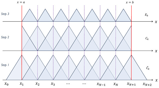 Figure 1. Procedure to build the dual cover mesh for the RKNMGM: Step 1 to generate the MC collection ; Step 2 to create the PC set ; and Step 3 to form the ME series .
 - Step 2
- Computing the intersection of each MC and the problem domain leads to the boundary PCs and , and the interior PCs , , which are illustrated as the bases of the overlapping triangles in the middle row in Figure 1;
- Step 3
- Computing the intersections of every adjacent pair of PCs gives the MEs: , , which are rendered as the triangle bases in the uppermost row in Figure 1.
3.2. Approximation
In the RKNMGM, the approximation of unknown variables is conducted over MCs, while the integration is calculated over MEs. Below, the approximation approach and integration formulations used in our method are described.
Given the dual cover mesh , we approximate the unknown variable over by a linear polynomial—that is,
where represents the linear polynomial basis function and denotes the coefficient. In the RKNMGM, the cover functions are the unknown to be determined. Thus, we will represent the coefficient by these cover functions below.
3.3. Weak Formulation
Since the system defined in Equations (5)–(7) is self-adjoint, the Galerkin weighted residual method can yield a symmetric system of equations. Consequently, we apply this method to transform Equation (5) into its weak form.
Choose the first-order Soblev space as the trial and test function space. Multiplying both sides of Equation (5) by any test function from , we obtain
where the notation represents the inner product in .
By applying integration by parts to the above equation, we arrive at
3.4. Semi-Discretization Scheme
Now, we derive the semi-discretization scheme from the weak form presented in Equation (16) by approximating and with Equation (12), i.e.,
Then, substituting the above formulations into Equation (16) leads to
where and are the mass matrix and stiffness matrix on , respectively, taking the formulas below
3.5. Time Integration Scheme
Next, we employ the TVD-RK2 [54] to solve the ODE problem of Equation (19) with the initial condition in Equation (6). As is symmetric positive definite, we can rewrite the semi-discretized system Equation (19) into the following general form:
where denotes the spatial operator.
For solving Equation (22) for , the TVD-RK2 scheme advances over a time step in the following two phases:
where represents . Particularly, contains the initial cover functions over and , respectively.
Since the cover function remains constant during a time step, we have , , and . Particularly, we take , where is the midpoint of . According to Equation (6), we have
As described in Equation (23), the TVD-RK2 scheme is an explicit time integration method. To ensure the computational stability, has to satisfy the CFL condition [54]:
in which contains all cover functions, and the norm indicates
3.6. Solution Restoration
Given as the solution of Equations (5)–(7) by the RKNMGM, we recover the solution of Equations (1)–(3) using the H-C transform once more.
First, use the central differential formula to compute , and Equation (4) becomes
where , and .
Since the collection comprises the numerical prediction on the MCs for Equations (1)–(3), we can use the NMM approximation provided in Equation (12) again to compute the solution at any point within the problem domain, i.e.,
Here, it worth noting that the weighting function possesses the Kronecker delta property in the ME .
4. Implementation Aspects
The numerical implementation of the RKNMGM for solving Equations (1)–(3) can be described in Algorithm 1.
In Line 10, Equation (23) is repeatedly executed, and it is computationally heavy to compute the inverse of the mass matrix .
As is symmetric positive definite, we employ Crout’s method, described in Algorithm 2, to compute .
Assume and as the exact solution and the prediction obtained by the RKNMGM at , respectively. The accuracy of the RKNMGM at can be measured by the relative error .
To further evaluate the global accuracy of our method, assume and to denote the exact solution and the prediction computed by the RKNMGM on all PCs. The global errors can be computed by
where the operators and represent the and norms, respectively.
| Algorithm 1: The RKNMGM scheme for solving Equations (1)–(3) |
| input: , , T, , , N output:  |
| Algorithm 2: Crout’s Method to Solve |
| Input: , N Output:  |
5. Validation Problems
Problem 1.
Below, we employ the RKNMGM scheme to numerically solve this problem. Using Equation (4), we transform the governing equation from Equation (1) into Equation (5), then convert the IC in Equation (31) into
and the homogeneous BC in Equation (7) becomes
As shown in Figure 2, we evaluate the convergence characteristics of the RKNMGM for this problem with when . Five different ME sizes, i.e., , are adopted. During the computations, we keep as the time step length. It can be observed from the figure that the global errors of the RKNMGM in the and consistently decrease while refining the spatial discretization, showcasing the good stability and convergence characteristic.
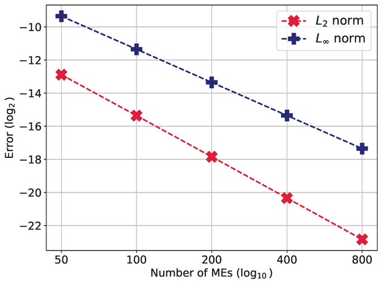
Figure 2.
Convergence performance of the RKNMGM for Problem 1.
Then, we examine the numerical solution of Problem 1 for different T while using a viscosity coefficient of . For each case, the parameters of the RKNMGM are set to be and . As depicted in Figure 3, we present the comparison of the solution curves produced by the RKNMGM against the exact solutions. The figure clearly indicates that the results from our method closely match the analytical formulations.
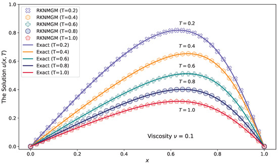
Figure 3.
RKNMGM results using , for Problem 1 with .
Table 1 presents the comparison of our results with exact solutions and those provided by the EFCGM [20] and the ENMCGM [40] at specific points and different times. Here, the EFCGM adopts 20 nodes with , the ENMCGM uses with , while the RKNMGM employs with . Compared with the EFCGM, our method needs finer discretization to achieve similar accuracy. However, the RKNMGM can strictly satisfy the homogeneous BC, which is challenging for the EFCGM due to using the MLS approximation. Besides, the EFCGM adopts the cubic spline weight function and utilizes Gaussian quadrature to calculate integrals, while our method employ a linear weight function and directly uses exact integration formulations. Compared with the ENMCGM, the present method requires much less MEs and smaller time step size, and the accuracy is better. These comparisons demonstrate that the efficiency and effectiveness of our method is on par with the EFCGM as well as the ENMCGM.

Table 1.
Numerical results and relative errors of different methods for Problem 1 ().
We then address this problem with a viscosity coefficient of using the RKNMGM, employing and . Figure 4 illustrates the comparison between our results and the exact solutions, indicating that the RKNMGM yields an outstanding agreement.
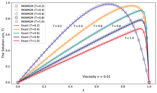
Figure 4.
RKNMGM results using , for Problem 1 with .
Table 2 provides a comparison of our results and those obtained from various numerical methods with the exact solution across different final times. In this test, the EFCGM adopts 50 nodes with , the ENMCGM uses with , while the RKNMGM employs with . The RKNMGM achieves similar accuracy to the EFCGM [20] while strictly enforcing the homogeneous BC, a challenge for the latter. Additionally, our method proves more accurate than the ENMCGM [40], even though the ENMCGM uses a finer spatial discretization and smaller time steps.
Table 2.
Numerical results and relative errors of different methods for Problem 1 ().
Before performing Algorithm 1 of the RKNMGM for the numerical analysis on this problem, we use Equation (4) to transform Equation (1) into Equation (5). Taking the parameter , we use the H-C transform to turn the IC in Equation (36) into
and adapt the homogeneous BC in Equation (7) into the Neumann BC in Equation (35).
As shown in Figure 5, the numerical results of the RKNMGM for Problem 2 are compared against the analytical solutions when . Diversified viscosity coefficients are considered, i.e., , and smaller leads to a more smoothly changing curve. During the computation, the time step size and ME size are set as and , respectively. A close agreement with the exact solutions can be found from Figure 5. It is indicated that our method is effective and stable.
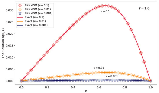
Figure 5.
The results of the RKNMGM against the exact solutions for Problem 2 when .
Then, we evaluate the convergence performance of the RKNMGM for Problem 2 in the case of . In Table 3, the global errors of the RKNMGM are demonstrated for different ME numbers and viscosity coefficients. During the computations, set , and diversified viscosity coefficients are adopted. It can be observed from the table that refining the dual cover mesh can give more accurate results for all of the cases. Besides, we can also find the phenomena that when the viscosity coefficient is reduced, the errors in both the and norm decrease.
Table 3.
Convergence behavior of the RKNMGM using and various ME numbers for Problem 2 with .
Next, we evaluate the results from the current method against those obtained from the ENMCGM [40] for Problem 2, focusing on two cases: and . During the test, both methods utilize 2000 MEs. The RKNMGM employs a time step of , while the ENMCGM uses . Table 4 presents the numerical results and the relative errors with respect to the analytical solution in Equation (37). The comparison reveals that the present method demonstrates greater accuracy and stability for both and . Further, the RKNMGM can use a larger time step size while achieving better computational performance.
Table 4.
Computing results and their relative errors obtained from different numerical methods for Problem 2 when .
Furthermore, the accuracy of the RKNMGM is compared with higher-order methods, such as the fifth-order FVM (FVCW) [15] and the collocation methods proposed by Ganaie [13] and Mittal [12]. In this test, these three references adopt the parameters and , while we choose and . Table 5 provides the exact solutions and numerical results on specific points. The data indicate that the RKNMGM demonstrates good accuracy, while it is slightly lower than that of the FVCW scheme. The latter benefits from the six-order Padé-based approximation. Our method outperforms the other two higher-order collocation methods in terms of accuracy. When using the same computing parameters as adopted in the other three methods, i.e., and , the relative error of our method is at all of the measured points. Although higher-order approaches exhibit impressive results, they may also demonstrate increased computational complexity. In contrast, the RKNMGM is more simple and easy to implement owing to using constant cover functions and linear weight functions. These comparisons highlight the effectiveness and efficiency of the RKNMGM, showcasing its competitive performance among various methods using higher-order approximation.
Table 5.
The results and relative errors of different numerical approaches for Problem 2 () when .
From Table 4 and Table 5, it is noteworthy that the present method exhibits almost uniform relative errors across different points, whereas the the other four methods do not possess this characteristic. This can be attributed to the time integration scheme adopted in this work, which maintains the TVD property, effectively suppressing numerical oscillations near sharp gradients.
Problem 3.
Next, consider Equations (1)–(3) on with
The exact solution of this problem is the same as Equation (32), but the coefficients and take the following formulation [4]:
where . Using Equation (4), Equation (1) is transformed into Equation (5), the IC in Equation (36) becomes , , and the BC in Equation (7) turns to be Equation (35).
For this example, we first assess the convergence performance of the RKNMGM using the time step size and various ME sizes—specifically, , , , , and . Here, we use a viscosity coefficient of and set the final time as . As illustrated in Figure 6, the global errors are presented in both and norms. The figure clearly demonstrates that our method converges as the discretization is refined.
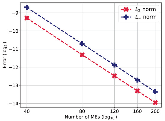
Figure 6.
Convergence study of the RKNMGM using and different ME numbers for Problem 3 in the case of and .
As shown in Figure 7 and Figure 8, the results of the RKNMGM align well with the exact solutions, corresponding to the diffusive coefficients and . In these computations, we adopt and . Notably, these curves exhibit similarities to those observed in Problem 1 owing to their similar exact solution formulations.
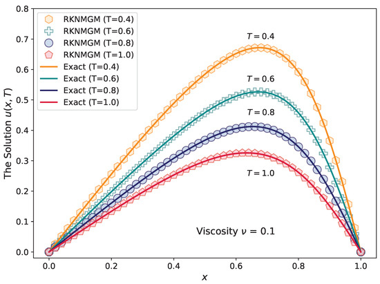
Figure 7.
RKNMGM results using , for Problem 3 with .
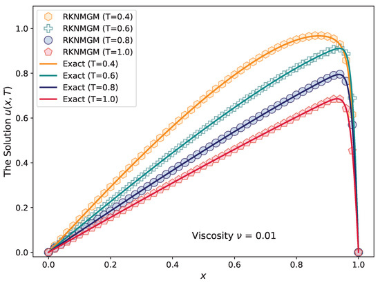
Figure 8.
RKNMGM results using , for Problem 3 with .
We further assess the accuracy of the RKNMGM at specific points for this example. For this test, the profile of the problem includes and . Table 6 presents a comparison of the numerical results obtained from our method with those solved by the fourth-order FDM [4] and the ENMCGM [40]. In the tests, the FDM uses with , the ENMCGM employs with , and we adopt with . It is evident that the RKNMGM can provide higher accuracy than the other two methods. Although our approach requires a finer mesh than the fourth-order FDM, it utilizes only constant cover functions and linear approximations, significantly reducing computational cost. Moreover, compared to the ENMCGM, which uses 2000 MEs, our method achieves greater accuracy with just 500 MEs, demonstrating the remarkable efficiency of the current approach.
Table 6.
Comparison of the results and relative errors obtained from different numerical methods for Problem 3 ().
Problem 4.
Consider the Burgers’ equation on , with Equation (42) at as the IC, i.e.,
In this case, the BC in Equation (3) becomes
Equation (41) provides the exact solution for this problem.
To numerically solve this problem with the RKNMGM, we use Equation (4) to convert Equation (1) into Equation (5) and transform the IC and BC into the following forms:
Figure 9 shows the convergence performance of the RKNMGM for Problem 4 with . Various spatial discretizations are considered, including cases with 50, 100, 200, 400, 800, and 1600 MEs. A consistent time step of was used throughout the computations. As depicted in the figure, the global errors of the RKNMGM decrease with increasing ME numbers, demonstrating clear convergence.
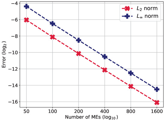
Figure 9.
The convergence behavior of the RKNMGM using and various spatial discretizations for Problem 4 in the case of and .
Table 7 compares the accuracy of the RKNMGM with other numerical methods, including the FEM [8] and our previously proposed ENMCGM scheme [40]. The ENMCGM utilizes 2000 MEs and employs for both of the cases and , while the present method utilizes and uses 400 MEs and 2000 MEs for and , respectively. Here, the computing settings used in the FEM have not been given by the author. The accuracy is evaluated in terms of global errors in both and norms for two cases of viscosity, and , with results presented for three different final times T. The RKNMGM demonstrates superior accuracy compared to the other two methods. This comparison shows the significant advantage of the RKNMGM in computational efficiency.
Table 7.
The global errors of the results computed by the RKNMGM compared with other numerical methods for Problem 4 with diversified cases of and T.
Figure 10 displays our results for Problem 4 with a viscosity coefficient of , compared to the exact solution. We use a time step size of and 200 MEs. As the final time T varies from 1.0 to 3.0, the curve becomes progressively smoother. The figure clearly demonstrates a close correspondence between our results and the exact solutions.
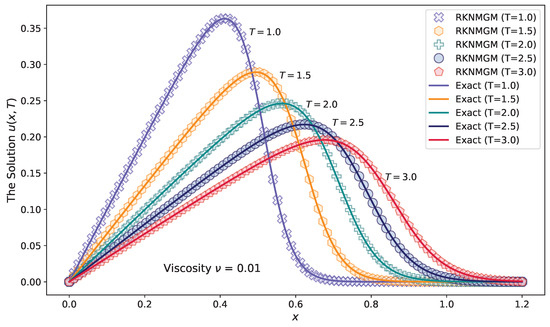
Figure 10.
RKNMGM results using and 200 MEs for Problem 4 with and different T against the exact solutions.
Additionally, Figure 11 presents our findings alongside the exact solution for this example with . In this case, we maintain a time step of while refining the spatial discretization to 2000 MEs. Noticeable steep gradients are evident in the curves for , and . Overall, it is evident that the results from the RKNMGM closely match the exact solutions.
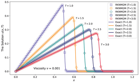
Figure 11.
RKNMGM results using and 2000 MEs for Problem 4 with .
6. Conclusions
The problem of the Burgers’ equation, as depicted in Equations (1)–(3), acts as a crucial framework for analyzing intricate nonlinear behaviors in fluid dynamics. In this paper, we proposed a Runge–Kutta numerical manifold Galerkin method (RKNMGM) specifically designed to solve this problem. This approach utilizes a dual cover mesh and PU-like weighted functions over manifold elements to enhance accuracy. To address the nonlinear advective term, we employed the H-C transform, shifting the original problem into a more manageable linear PDE. We conducted several benchmark numerical tests to evaluate the performance of the RKNMGM. Based on the numerical results, several notable advantages of the RKNMGM are worth highlighting, as follows:
- (1)
- The H-C transform simplifies the Burgers’ equation, significantly reducing the complexity of solving the original equation while preserving essential physical characteristics. The solution to the original problem can be conveniently recovered from that of the transformed problem using the H-C transform once again.
- (2)
- By adopting the dual cover approximation with constant cover functions and linear weight functions, computational costs are reduced while Dirichlet boundary condition can be accurately imposed. Additionally, integrals over manifold elements are computed using simplex integration formulas instead of Gaussian quadrature, further enhancing accuracy and efficiency.
- (3)
- We introduced the fully explicit TVD-RK2 scheme for temporal discretization in the NMM. Although both the TVD-RK2 and the Crank–Nicolson method have second-order accuracy, the TVD property possessed in the former one brings our present method an advantage in suppressing numerical oscillations, as evidenced in the numerical experiments.
- (4)
- The final computational formulation, derived from the Galerkin weak form, results in a symmetric mass matrix, whose inverse can be efficiently obtained using the Crout method. This facilitates implementation and parallelization of the RKNMGM.
- (5)
- Our numerical results for the Burgers’ equation under diversified initial condition values were thoroughly compared with exact solutions and other numerical methods. These comparisons demonstrate that our method effectively captures steep gradients, even for very small viscosity coefficients.
It is important to acknowledge that this study concentrates exclusively on the one-dimensional Burgers’ equation. In our future research, we look forward to extending our exploration to high-dimensional cases, which will broaden the applicability of the findings presented here. This investigation will enable us to address more complex PDEs that are significant in the realm of fluid dynamics.
Author Contributions
Conceptualization and Methodology, Y.S.; Software and Original draft preparation, Q.C.; Validation and Data Analysis, T.C.; Visualization, L.Y. All authors have read and agreed to the published version of the manuscript.
Funding
This research was supported by the Natural Science Foundation of Shaanxi Province of China (Grant No. 2024JC-YBMS-014) and the Research Foundation for the Doctoral Program of Shaanxi University of Technology (Grant No. SLGQD2017-08).
Data Availability Statement
Profiles presented in the study are included in the article.
Conflicts of Interest
The authors declare no conflicts of interest.
References
- Burgers, J.M. A mathematical model illustrating the theory of turbulence. Adv. Appl. Mech. 1948, 1, 171–199. [Google Scholar]
- Cole, J.D. On a quasi-linear parabolic equation occurring in aerodynamics. Quart. Appl. Math. 1951, 9, 225–236. [Google Scholar] [CrossRef]
- Wood, W. An exact solution for Burger’s equation. Commun. Numer. Meth. Eng. 2006, 22, 797–798. [Google Scholar] [CrossRef]
- Hassanien, I.; Salama, A.; Hosham, H.A. Fourth-order finite difference method for solving Burgers’ equation. Appl. Math. Comput. 2005, 170, 781–800. [Google Scholar] [CrossRef]
- Yağmurlu, M.; Gagir, A. A finite difference approximation for numerical simulation of 2D viscous coupled burgers equations. Math. Sci. Appl. E-Notes 2022, 10, 146–158. [Google Scholar] [CrossRef]
- Kaur, R.; Kukreja, V.; Parumasur, N.; Singh, P. Two different temporal domain integration schemes combined with compact finite difference method to solve modified Burgers’ equation. Ain Shams Eng. J. 2022, 13, 101507. [Google Scholar] [CrossRef]
- Vandandoo, U.; Zhanlav, T.; Chuluunbaatar, O.; Gusev, A.; Vinitsky, S.; Chuluunbaatar, G. Higher-Order Finite-Difference Methods for the Burgers’ Equations. In High-Order Finite Difference and Finite Element Methods for Solving Some Partial Differential Equations; Springer Nature: Cham, Switzerland, 2024; pp. 35–67. [Google Scholar]
- Dogan, A. A Galerkin finite element approach to Burgers’ equation. Appl. Math. Comput. 2004, 157, 331–346. [Google Scholar] [CrossRef]
- Chen, H.; Jiang, Z. A characteristics-mixed finite element method for Burgers’ equation. J. Appl. Math. Comput. 2004, 15, 29–51. [Google Scholar] [CrossRef]
- Saka, B.; Dağ, İ. A numerical study of the Burgers’ equation. J. Franklin Inst. 2008, 345, 328–348. [Google Scholar] [CrossRef]
- Dağ, İ.; Irk, D.; Saka, B. A numerical solution of the Burgers’ equation using cubic B-splines. Appl. Math. Comput. 2005, 163, 199–211. [Google Scholar] [CrossRef]
- Mittal, R.; Jain, R. Numerical solutions of nonlinear Burgers’ equation with modified cubic B-splines collocation method. Appl. Math. Comput. 2012, 218, 7839–7855. [Google Scholar] [CrossRef]
- Ganaie, I.A.; Kukreja, V.K. Numerical solution of Burgers’ equation by cubic Hermite collocation method. Appl. Math. Comput. 2014, 237, 571–581. [Google Scholar] [CrossRef]
- Arar, N.; Deghdough, B.; Dekkiche, S.; Torch, Z.; Nagy, A. Numerical Solution of the Burgers’ Equation Using Chelyshkov Polynomials. Int. J. Appl. Comput. Math. 2024, 10, 33. [Google Scholar] [CrossRef]
- Guo, Y.; Shi, Y.f.; Li, Y.m. A fifth-order finite volume weighted compact scheme for solving one-dimensional Burgers’ equation. Appl. Math. Comput. 2016, 281, 172–185. [Google Scholar] [CrossRef]
- Shahabi, A.; Ghiassi, R. A robust second-order godunov-type method for Burgers’ equation. Int. J. Appl. Comput. Math. 2022, 8, 82. [Google Scholar] [CrossRef]
- Xin, J.; Flaherty, J. Implicit time integration of hyperbolic conservation laws via discontinuous Galerkin methods. Int. J. Numer. Methods Biomed. Eng. 2011, 27, 711–721. [Google Scholar] [CrossRef]
- Zhang, R.P.; Yu, X.J.; Zhao, G.Z. Modified Burgers’ equation by the local discontinuous Galerkin method. Chin. Phys. B 2013, 22, 030210. [Google Scholar]
- Hutridurga, H.; Kumar, K.; Pani, A.K. Discontinuous Galerkin methods with generalized numerical fluxes for the Vlasov-viscous Burgers’ system. J. Sci. Comput. 2023, 96, 7. [Google Scholar]
- Zhang, X.H.; Ouyang, J.; Zhang, L. Element-free characteristic Galerkin method for Burgers’ equation. Eng. Anal. Boundary Elem. 2009, 33, 356–362. [Google Scholar] [CrossRef]
- Zhang, L.; Ouyang, J.; Wang, X.; Zhang, X. Variational multiscale element-free Galerkin method for 2D Burgers’ equation. J. Comput. Phys. 2010, 229, 7147–7161. [Google Scholar] [CrossRef]
- Ma, L.; Zhao, L.; Wang, X. An iteration-free semi-Lagrangian meshless method for Burgers’ equations. Eng. Anal. Boundary Elem. 2023, 150, 482–491. [Google Scholar] [CrossRef]
- Hashemian, A.; Shodja, H.M. A meshless approach for solution of Burgers’ equation. J. Comput. Appl. Math. 2008, 220, 226–239. [Google Scholar] [CrossRef]
- Xie, H.; Li, D. A meshless method for Burgers’ equation using MQ-RBF and high-order temporal approximation. Appl. Math. Modell. 2013, 37, 9215–9222. [Google Scholar] [CrossRef]
- Shyaman, V.; Sreelakshmi, A.; Awasthi, A. A higher order implicit adaptive finite point method for the Burgers’ equation. J. Differ. Equ. Appl. 2021, 29, 235–269. [Google Scholar] [CrossRef]
- Shi, G.H. Manifold method of material analysis. In Proceedings of the Transactions of the 9th Army Conference on Applied Mathematics and Computing, US Army Research Office Minneapolis, Minneapolis, MN, USA, 21–25 October 1991; Volume 92. [Google Scholar]
- Lin, J.S. A mesh-based partition of unity method for discontinuity modeling. Comput. Methods Appl. Mech. Eng. 2003, 192, 1515–1532. [Google Scholar] [CrossRef]
- Zheng, H.; Liu, Z.; Ge, X. Numerical manifold space of Hermitian form and application to Kirchhoff’s thin plate problems. Int. J. Numer. Meth. Eng. 2013, 95, 721–739. [Google Scholar] [CrossRef]
- Zheng, H.; Wang, F. The numerical manifold method for exterior problems. Comput. Methods Appl. Mech. Eng. 2020, 364, 112968. [Google Scholar] [CrossRef]
- Guo, H.; Cao, X.; Liang, Z.; Lin, S.; Zheng, H.; Cui, H. Hermitian numerical manifold method for large deflection of irregular Föppl-von Kármán plates. Eng. Anal. Bound. Elem. 2023, 153, 25–38. [Google Scholar] [CrossRef]
- Tan, F.; Tong, D.; Liang, J.; Yi, X.; Jiao, Y.Y.; Lv, J. Two-dimensional numerical manifold method for heat conduction problems. Eng. Anal. Bound. Elem. 2022, 137, 119–138. [Google Scholar] [CrossRef]
- Ji, X.; Zhang, H.; Han, S. Transient heat conduction modeling in continuous and discontinuous anisotropic materials with the numerical manifold method. Eng. Anal. Bound. Elem. 2023, 155, 518–527. [Google Scholar] [CrossRef]
- Ning, Y.; Lu, Q.; Liu, X. Fracturing failure simulations of rock discs with pre-existing cracks by numerical manifold method. Eng. Anal. Bound. Elem. 2023, 148, 389–400. [Google Scholar] [CrossRef]
- Zhang, N.; Zheng, H.; Li, X.; Wu, W. On hp refinements of independent cover numerical manifold method—some strategies and observations. Sci. China Technol. Sci. 2023, 66, 1335–1351. [Google Scholar] [CrossRef]
- Zhang, L.; Kong, H.; Zheng, H. Numerical manifold method for steady-state nonlinear heat conduction using Kirchhoff transformation. Sci. China Technol. Sci. 2024, 67, 992–1006. [Google Scholar] [CrossRef]
- Tong, D.; Yi, X.; Tan, F.; Jiao, Y.; Liang, J. Three-dimensional numerical manifold method for heat conduction problems with a simplex integral on the boundary. Sci. China Technol. Sci. 2024, 67, 1007–1022. [Google Scholar] [CrossRef]
- Zhang, Z.; Zhang, X.; Yan, J. Manifold method coupled velocity and pressure for Navier–Stokes equations and direct numerical solution of unsteady incompressible viscous flow. Comput. Fluids 2010, 39, 1353–1365. [Google Scholar] [CrossRef]
- Lin, S.; Cao, X.; Zheng, H.; Li, Y.; Li, W. An improved meshless numerical manifold method for simulating complex boundary seepage problems. Comput. Geotech. 2023, 155, 105211. [Google Scholar] [CrossRef]
- Su, H.; Lin, S.; Xie, Z.; Gong, Y.; Qi, Y. Fundamentals and progress of the manifold method based on independent covers. Sci. China Technol. Sci. 2024, 67, 966–991. [Google Scholar] [CrossRef]
- Sun, Y.; Chen, Q.; Chen, T.; Yong, L. Explicit Numerical Manifold Characteristic Galerkin Method for Solving Burgers’ Equation. Axioms 2024, 13, 343. [Google Scholar] [CrossRef]
- Hopf, E. The partial differential equation ut + uux = μuxx. Commun. Pure Appl. Math. 1950, 3, 201–230. [Google Scholar] [CrossRef]
- Fahmy, E.; Raslan, K.R.; Abdusalam, H. On the exact and numerical solution of the time-delayed Burgers equation. Int. J. Comput. Math. 2008, 85, 1637–1648. [Google Scholar] [CrossRef]
- Kudryashov, N.A.; Sinelshchikov, D.I. Exact solutions of equations for the Burgers hierarchy. Appl. Math. Comput. 2009, 215, 1293–1300. [Google Scholar] [CrossRef]
- Ohwada, T. Cole-Hopf transformation as numerical tool for the Burgers equation. Appl. Comput. Math 2009, 8, 107–113. [Google Scholar]
- Cordero, A.; Franques, A.; Torregrosa, J.R. Numerical solution of turbulence problems by solving Burgers’ equation. Algorithms 2015, 8, 224–233. [Google Scholar] [CrossRef]
- Uddin, M.; Ali, H. The space–time kernel-based numerical method for Burgers’ equations. Mathematics 2018, 6, 212. [Google Scholar] [CrossRef]
- Al-shimmary, A.F.; Kareem, S.; Hussain, A.K. A new approach to solve Burges’ equation using Runge-Kutta 6th order method based on Cole-Hopf transformation. J. Eng. Appl. Sci. 2020, 15, 2362–2369. [Google Scholar]
- Abd-Elhameed, W.M. Novel expressions for the derivatives of sixth kind Chebyshev polynomials: Spectral solution of the non-linear one-dimensional Burgers’ equation. Fractal Fract. 2021, 5, 53. [Google Scholar] [CrossRef]
- Savović, S.; Ivanović, M.; Min, R. A Comparative Study of the Explicit Finite Difference Method and Physics-Informed Neural Networks for Solving the Burgers’ Equation. Axioms 2023, 12, 982. [Google Scholar] [CrossRef]
- Singh, G.; Singh, I.; AlDerea, A.M.; Alanzi, A.M.; Khalifa, H.A.E.W. Solutions of (2+1)-D & (3+1)-D Burgers Equations by New Laplace Variational Iteration Technique. Axioms 2023, 12, 647. [Google Scholar] [CrossRef]
- Öziş, T.; Aksan, E.; Özdeş, A. A finite element approach for solution of Burgers’ equation. Appl. Math. Comput. 2003, 139, 417–428. [Google Scholar] [CrossRef]
- Guo-Zhong, Z.; Xi-Jun, Y.; Di, W. Numerical solution of the Burgers’ equation by local discontinuous Galerkin method. Appl. Math. Comput. 2010, 216, 3671–3679. [Google Scholar] [CrossRef]
- Mukundan, V.; Awasthi, A. Efficient numerical techniques for Burgers’ equation. Appl. Math. Comput. 2015, 262, 282–297. [Google Scholar] [CrossRef]
- Shu, C.W. Total-variation-diminishing time discretizations. SIAM J. Sci. Stat. Comput. 1988, 9, 1073–1084. [Google Scholar] [CrossRef]
- Shi, G.H. Modeling dynamic rock failure by discontinuous deformation analysis with simplex integrations. In Proceedings of the ARMA North America Rock Mechanics Symposium, Austin, TX, USA, 1–3 June 1994. [Google Scholar]
- Lin, S.; Xie, Z. A new recursive formula for integration of polynomial over simplex. Appl. Math. Comput. 2020, 376, 125140. [Google Scholar] [CrossRef]
Disclaimer/Publisher’s Note: The statements, opinions and data contained in all publications are solely those of the individual author(s) and contributor(s) and not of MDPI and/or the editor(s). MDPI and/or the editor(s) disclaim responsibility for any injury to people or property resulting from any ideas, methods, instructions or products referred to in the content. |
© 2024 by the authors. Licensee MDPI, Basel, Switzerland. This article is an open access article distributed under the terms and conditions of the Creative Commons Attribution (CC BY) license (https://creativecommons.org/licenses/by/4.0/).