Enhancing Supply Chain Sustainability and Reliability Through WSM and TOPSIS: A Symmetrical Real-World Case Study

Abstract

Large corporations have recently demonstrated an increasing propensity to enhance the sustainability and reliability of their supply chains in order to comply with environmental regulations and improve customer satisfaction through on-time demand fulfillment. There are two phases to this study: mathematical modeling and model solution using precise techniques. In the first step, a mixed-integer linear programming model is developed. This model is an improvement of an existing supply chain model. Further, our suggested strategy is verified by using numerical data based on three criteria and four suppliers. The goals of the proposed model are to maximize supply chain reliability, economic profit, and social responsibilities by taking suppliers’ priorities into account. Modeled as a mixed-integer linear programming problem, the constraints on the problem include budget, emission, demand, allocation, facility, and shipping capacity. Power symmetry and information symmetry are incorporated in order to perform symmetric analysis. The weighted sum method (WSM) and the technique for order of preference by similarity to ideal solution (TOPSIS) are the two methods used in the second step of solving the model to identify the best supplier. In order to evaluate how well the proposed methodology was applied, a practical case was considered and implemented.

1. Introduction

Supply chain designs that overlook sustainability, risk, or multimodality may jeopardize long-term competitiveness because these components are essential given the intense global competition and exceedingly demanding customers. Sustainable development is essential when social, environmental, and economic factors are taken into account.

Reliability (R_D,C,L) is the probability that the sustainable supply chain network (SSCN) will meet the supplier’s demand D, budget, and production capacity while maintaining the supplier’s sustainability level L in the SSCN. Supply chain network design (SCND) sustainability and reliability serve as a competitive advantage that increases customer satisfaction and keeps businesses afloat.

A triple-C (cease-control-combine) solution is suggested for the management of supply chain in the auto industry, [1]. Sometimes multiple regression analysis was also used by for sustainable supply chain management and performance [2]. Green purchasing, eco-design and reverse supply chain are the actions that corporate entities should take to advance sustainable development [3]. The three interconnected dimensions of inclusivity, scope, and disclosure are at the heart of the sustainable evaluation and verification (SEV) framework, which describes how supply chain operations may choose important metrics, gather and analyze data, and then confirm the accuracy, dependability, and materiality of any data and information that is produced [4]. Use of interval-valued triangular fuzzy numbers to represent linguistic preferences incorporating an expert team with industrial experience was also suggested [5]. Additionally, multi-criteria decision making was used to evaluate the hierarchical structure in determining the ranking of tradeoffs and competitive priorities. Booming development of the omni channel were recognized for designing supply chain networks with multiple distribution channels [6]. Using fuzzy preference programming and the FTOPSIS method a hybrid hierarchical decision-making model was proposed in order to select an optimal supplier [7]. The sustainability risks for management of supply chain were classified into five dimensions of sustainable development, including environmental, social, economic, technical, and institutional dimensions [8]. Uncertain parameters and component reliability were considered in a dynamic supply chain with multiple products [9]. The reliability technique is used to address real-world uncertainties in cost parameters, whereas supply and demand factors are regarded as uncertain variables [10]. A statistical technique was described that calculates the supply chain’s overall reliability rate in addition to the reliability rate of each component in the system [11]. In order to understand data-driven sustainable supply chain management performance, big data were used to analyze the relationships between the attributes [12]. A novel aim function that optimizes the reliability of product distribution is expanded in order to guarantee the network’s responsiveness. The network is also protected from disturbances by a novel reliability method [13]. Different relationships were observed among sustainability, reliability, and multimodality [14]. MATLAB coding techniques are combined with generalized TOPSIS, WSM, and Weighted Product Method to get the best type of laser for specific surgeries [15]. The forward supply chain in supply chain consists of suppliers, manufacturers, warehouses, and customer, on the other hand the reverse supply chain consists of collection centers, repair services, and disposal facilities [16]. TOPSIS method can deal with both qualitative and quantitative criteria, but the method may be sensitive to the criteria’s weight [17]. With the assistance of AHP, TOPSIS, and WSM, single valued neutrosophic sets were used as a comparative model in the comparative analysis to validate the model [18]. A conceptual framework is also presented that highlights the causes and effects of optimizing production in the materials science and engineering sector using the TOPSIS technique, which can raise Supply Chains’ competitiveness [19]. Sustainable supplier selection specifically meant to encourage suppliers to lower their carbon footprint during the sourcing process, improving their environmental policies as green suppliers [20]. The supply chain’s overall reliability was maximized on the basis of structural reliability theory [21]. Reliability and sustainability standards were looked in the process of choosing suppliers for a supply chain that includes wholesalers, suppliers, and a central warehouse [22]. In order to protect the environment, a multi-item, multi-objective inventory model was suggested with back-ordered quantity and green investment [23]. Using both symmetric (PLS-SEM) and asymmetric (fsQCA) methodologies and utilizing survey data from 166 companies involved in Ghana’s downstream petroleum industry, the performances were investigated [24]. An optimization method based on the unpredictability of bioenergy demand and the disruption in the bio-refinery was used to design a robust and sustainable biomass supply network [25]. To address the single-objective model, an imperialist competitive algorithm (ICA) was created [26]. A robust fuzzy optimization model with objectives of maximizing profit, number of jobs, and reliability was developed considering environmental emissions as one of the constraint [27]. A novel algorithm for reliability computation is also developed incorporating supplier sustainability into reliability assessment [28]. The adaptive m-objective ε-constraint approach was employed to solve the mathematical model and determine the optimal Pareto fronts [29]. They took assumptions of a five-level supply chain network with disruption experiences. In other work, results of the augmented epsilon constraint and normalized normal constraint methods were compared using the four criteria of run time (RT), mean ideal distance (MID), diversification metric (DM), and standard deviation metric (SDM) [30]. In the above work, reliability was not optimized using TOPSIS and WSM methods.

In this paper, we have tried to optimize profit, social responsibility, and reliability by advancing the assumptions and using WSM and TOPSIS techniques to improve the sustainability and reliability of the proposed supply chain. We included disposal cost in our proposed model to identify the cost of disposal, which is the sum of money that a company or an individual must pay in order to get rid of a waste product or asset.

2. Problem Description

Prioritizing consumer satisfaction and social responsibility, the current research models a reliable, affordable, and closed-loop supply chain network design problem mathematically. Supply chains aim to be highly reliable, socially responsible, and profitable. In addition to making strategic decisions about the placement of possible facilities like production, distribution, collection, and recycling centers, supply chains can also make tactical decisions about the rate at which materials and goods move through the chain. To achieve this, a mixed-integer linear programming (MILP) model has been created. The suggested model can be used in many different industries where it is socially responsible to collect end-of-life products from customers, such as pharmaceuticals, dairy products, non-rechargeable batteries, car tires, and others. The proposed supply chain network includes manufacturers, distributors, suppliers, marketplaces, and consumers for recycled raw materials, recycling and collection facilities, energy recovery centers, and disposal sites in the reverse chain. In this structure, customers or final consumers are the main demand source. It was predicated on the idea that each chain level’s constituent parts do not have any unique relationships. Put differently, there is no exchange of goods between subsystems, and each component functions independently of the others. Customers and suppliers have fixed locations. Furthermore, three distinct capacities (small, medium, and large) for manufacturing, distribution, collection, and recycling centers can be established, with various fixed setup costs corresponding to each capacity level.

In the direct chain, producers create goods that are shipped to distribution centers using a specific mix of raw materials that they buy from suppliers. The responsibility for storing the goods and getting them to final customers rests with the distribution centers [31]. Used goods are sent back from demand centers to collection centers in the reverse supply chain [32,33]. There, they are inspected and sorted into three quality categories: high value, low value, and worthless (based on the amount of time used). Based on the materials used in the recycling process, the recycled raw materials are divided into two categories: raw materials appropriate for secondary market sales as well as production-useful raw materials. Heterogeneous vehicles transport goods and raw materials between various supply chain levels. Failure modes are established for transportation facilities, routes, and trucks in order to take into consideration the inherent conditions of the issue. Within the model, it is discussed how these failures affect the supply chain’s reliability. Every supply chain facility is given a reliability index, which indicates the likelihood of proper operation without a breakdown in a specific amount of time. This index is dependent on the level of flexibility, design strength, and investment amount. Facilities that are more adaptable are more dependable. Furthermore, the storage systems and separation capabilities of distribution and collection centers play a major role in their dependability. The more responsive they are, the more trustworthy they are. The technologies used in production, product storage, and material recycling vary amongst facilities. Given the distance between the locations, the likelihood that the vehicles being used will malfunction and the communication routes are taken into account when measuring the reliability of transportation activities.

2.1. Research Implementation Methodology

Two fundamental processes are needed to solve an optimization problem: mathematical modeling and model solving. The completion of each step is necessary for optimization, as they are complementary to one another. Furthermore, different approaches to a multi-objective problem frequently result in different solutions. Therefore, for multi-objective methods, providing diverse solutions and achieving convergence in Pareto solutions are two distinct and somewhat competing goals. Determining the appropriate multi-objective approaches, solving the problem model with the determined approaches, identifying the appropriate criteria for evaluating the approaches, evaluating and comparing the approaches, and selecting the best approach for solving the sustainable and reliable SCND problem are all necessary steps in selecting the appropriate solution method for the current research problem.

2.2. Notation List

The problem is represented mathematically in this section. By combining comparable symbols, parameters, and variables for easier reference,

Table 1. Definition of variables, parameters and symbols.

Category	Symbol	Description
		Sets
Main	I	Suppliers, iϵ I
	J	Potential production centers, j ϵ J
	D	Potential distribution centers, d ϵ D
	E	Primary market, e ϵ E
	C	Potential collection centers, c ϵ C
	M	Potential recycling centers, m ϵ M
	K	Potential remanufacturing center, k ϵ K
	H	Secondary market for recycled raw material, h ϵ H
	F	Landfill centers, f ϵ F
	B	Energy recovery centers, b ϵ B
	A	Raw materials, a ϵ A
	R	Products, r ϵ R
	L	Materials used in recycling process, l ϵ L
	G	Technologies in production center, g ϵ G
	V	Vehicle, v ϵ V
	U	Usable capacity, u ϵ U
	P	Period, p ϵ P
Hybrid	N	Network nodes, N ϵ {i,j,k,e,c,m,k,b,f,h}
	$\mathsf{\delta }$	$\mathrm{Network} \mathrm{arcs}, \mathsf{\delta }\left(\mathrm{x},\mathrm{y}\right) \mathsf{ϵ}\left\{\begin{array}{c}1:\left(i,j\right),{\mathsf{\delta }}_2:\left(\mathrm{j},\mathrm{m}\right),{\mathsf{\delta }}_3:\left(\mathrm{m},\mathrm{h}\right),{\mathsf{\delta }}_4:\left(\mathrm{j},\mathrm{d}\right),\\ {\mathsf{\delta }}_5:\left(\mathrm{d},\mathrm{e}\right),{\mathsf{\delta }}_6:\left(\mathrm{e},\mathrm{c}\right),{\mathsf{\delta }}_7:\left(\mathrm{c},\mathrm{m}\right)\\ ,{\mathsf{\delta }}_8:\left(\mathrm{c},\mathrm{b}\right),{\mathsf{\delta }}_9:\left(\mathrm{c},\mathrm{f}\right),{\mathsf{\delta }}_{10}:\left(\mathrm{m},\mathrm{k}\right),{\mathsf{\delta }}_{11}:(\mathrm{k},\mathrm{d})\end{array}\right.$
	${\mathsf{\delta }}^{\prime }$	$\mathrm{Arcs} \mathrm{for} \mathrm{carrying} \mathrm{raw} \mathrm{materials}, {\mathsf{\delta }}^{\prime }$$\subset \mathsf{\delta }$$, {\mathsf{\delta }}^{\prime }\mathsf{ϵ}\left\{{\mathsf{\delta }}_1,{\mathsf{\delta }}_2,{\mathsf{\delta }}_3\right\}$
	${\mathsf{\delta }}^{″}$	$\mathrm{Arcs} \mathrm{for} \mathrm{carrying} \mathrm{products},{\mathsf{\delta }}^{″} \mathrm{\subset } \mathsf{\delta }$$,{\mathsf{\delta }}^{″}\mathsf{ϵ}\left\{{\mathsf{\delta }}_4,{\mathsf{\delta }}_5,{\mathsf{\delta }}_6,{\mathsf{\delta }}_7,{\mathsf{\delta }}_8,{\mathsf{\delta }}_9,{\mathsf{\delta }}_{10},{\mathsf{\delta }}_{11}\right\}$
		Parameters
Prices	$C_{er}^p$	The price at which a single unit of product r unit is sold in the primary market e during a given period p
	$C_{br}^p$	The selling price in the energy recovery center (b) for a single unit of returned product (r) during the period p
	$C_{ha}^p$	The price at which one unit of recycled raw material (a) is sold for during a specific time period (p) in the secondary market (h)
	$C_{hk}^p$	The price at which one unit of remanufacturing product (k) is sold for during a specific time period (p) in the secondary market (h)
Fixed Costs	$F_j^{gu}$	Fixed expenses for establishing a single production facility j with capacity u and technology g
	$F_d^u$	Putting up a single distribution center at a fixed cost of d and capacity level of u
	$F_c^u$	To create a single collection center (c) with a capacity level of u, a predefined amount will be needed.
	$F_k^u$	To create a single remanufacturing center (k) with a capacity level of u, a predefined amount will be needed
	$F_m^{lu}$	Predetermined establishment costs for a single recycling facility m with material l and capacity u
	$F_{ia}^p$	The one-time cost associated with entering into an agreement with a supplier i to provide raw material a for a specific time frame p
	$F_v^p$	Fixed cost for vehicle v for time p
	Θ	Fixed cost of reducing carbon dioxide emissions
Unit Costs	${BC}_{ia}^p$	The cost of purchasing one fresh input (a) unit from supplier i for a specific amount of time (p)
	${RC}_a^p$	Reductions on expenses as a result of recycling one raw material (a) unit over a specified amount of time p
	${PC}_{jr}^{gp}$	Cost over time of using technology g to produce a single product r in the manufacturing facility j at time p
	${DC}_{dr}^p$	Price of single product r’s distribution over time (p) at distribution center d
	${HC}_{dr}^p$	Cost of upkeep for a single product unit (r) at distribution center (d) for time interval (p)
	${EC}_{er}^p$	Penalties for not having one unit of product r during time p
	${OEC}_{er}^p$	A non-collection penalty from the customer e for one returned product (r) unit over the course of time p
	${CC}_{cr}^p$	The total cost over time p of packing and sorting a single came-back goods (r) unit at the pickup center c
	${OCC}_{cr}^p$	The purchase incentive’s cost and the goods (r) that is being retrieved from the pickup facility (c) within a specified time frame (p)
	${MC}_{mr}^{lp}$	The price of reusing one returned product unit (r) over a specified time period (p) at a recycling facility (m) using material (l)
	${FC}_{fr}^p$	Cost of destroying, over a given period of time p, one unit of returned product r at the destruction center f
	$V_v^p$	The price of one liter of fuel for a vehicle v over time p
	$F^p$	Driver’s pay for an hour of driving over a given period of time p
Capacities	${Cap}_{ia}$	The supplier i’s ability to supply unprocessed materials a
	${Cap}_j^{gu}$	Capacity of production center j using technology g and capacity level u
	${Cap}_d^u$	Capacity of distribution center d with capacity level u
	${VCap}_d^u$	The storage capacity of distribution center d at capacity level u
	${Cap}_c^u$	Capacity of collection center c with capacity level u
	${Cap}_m^{lu}$	Disposal and reusing facility m ability with substance l and capacity u
	${Cap}_k^u$	Capacity of remanufacturing center k with capacity level u
	${WCap}^v$	Weight capacity for vehicle v
	${VCap}^v$	Capacity of volume for type of vehicle v
Carbon Dioxide	${CO}_2^{GOV}$	$\mathrm{The} \mathrm{government}-\mathrm{allowed} \mathrm{amount} \mathrm{of} {CO}_2$ emissions for the supply chain network
	$E_j^{gu}$	$\mathrm{Fixed} {CO}_2$ emissions from establishing a production center j with a capacity of u and utilizing technology g
	$E_d^u$	$\mathrm{Fixed} {CO}_2$ emissions resulting from the establishment of a distribution center d at a capacity level of u
	$E_c^u$	$\mathrm{Fixed} {CO}_2$ emissions as a result of building a collection center c with a capacity level of u
	$E_m^{lu}$	$\mathrm{Predetermined} {CO}_2$ emissions from establishing a disposal and reusing facility m with substance l and capacity u
	$E_k^u$	$\mathrm{Fixed} {CO}_2$ emissions as a result of building a remanufacturing center k with a capacity level of u
	${\mu }^j$	${CO}_2$ emissions rate per unit of energy used (g/kwh)
	${\mu }^l$	$\mathrm{Rate} \mathrm{of} {CO}_2$$\mathrm{emission} \mathrm{for} \mathrm{one} \mathrm{liter} \mathrm{of} \mathrm{fuel} \mathrm{consumption} \left(\mathrm{g}/\mathrm{L}\right)$
Energy and Fuel	${EP}_r^g$	Energy consumption needed to create single unit of a goods r using technology g (kWh)
	${ED}_r$	$\mathrm{Consumption} \mathrm{of} \mathrm{energy} \mathrm{for} \mathrm{distribution} \mathrm{of} \mathrm{one} \mathrm{unit} \mathrm{of} \mathrm{product} \mathrm{r} \left(\mathrm{k}\mathrm{W}\mathrm{h}\right)$
	${EC}_r$	Energy used to pick up one unit of retrieved merchandise r (kWh)
	${EM}_a^l$	Energy used to recycle a single unit of raw material (a) using a substance l (kWh)
	${EB}_r$	The amount of energy needed to recycle one unit of a retrieved good r (kWh)
	${EF}_r$	$\mathrm{Energy} \mathrm{Consumption} \mathrm{for} \mathrm{buying} \mathrm{per} \mathrm{unit} \mathrm{of} \mathrm{returned} \mathrm{product} \mathrm{r} \left(\mathrm{k}\mathrm{W}\mathrm{h}\right)$
	${FU1}_v$	Consumption of fuel for one kilometer traveling by the vehicle v in no-load mode (L)
	${FU2}_v$	Fuel consumption for a vehicle v traveling one kilometer versus each unit of load (L)
Jobs	${\theta }_{job}$	Significance coefficient for newly created jobs
	${job}_j^{gu}$	Prospects for employment as a result of setting up a production center j with capacity u and technology g
	${job}_d^u$	Employment generated by building a distribution center d with capacity level u
	${job}_c^u$	Opportunities for employment as a result of building a collection center c with an u capacity
	${job}_m^{lu}$	The construction of a recycling facility m with material l and capacity level u could potentially create jobs
	${job}_k^u$	Opportunities for employment as a result of building a remanufacturing center k with an u capacity
	${\eta }_j$	Unemployment rate at the production center j
	${\eta }_d$	Unemployment rate in distribution center d
	${\eta }_c$	Unemployment rate in collection center c
	${\eta }_m$	The recycling center m’s unemployment rate
	${\eta }_k$	Unemployment rate in remanufacturing center k
	$jp$	Varying rate of employment creation for a single operational hour
Occupational injuries	${\theta }_{lpc}$	Importance coefficient of sick leave
	${lpc}_j^{gu}$	Workplace injuries as a function of capacity level (u), technology (g), and production center (j) (days)
	${lpc}_d^u$	Workplace injuries as a result of building a distribution center d with a capacity of u (days)
	${lpc}_c^u$	Workplace injuries brought on by the establishment of a collection center (c) with a u (days) capacity
	${lpc}_m^{lu}$	Workplace injuries as a result of the material l, the capacity level u, and the establishment of the recycling center m (days)
	${lpc}_k^u$	Workplace injuries as a result of building a remanufacturing center k with a capacity of u (days)
	$l_p$	Varying rate of occupational injuries for each operational hour
Reliability	${\lambda }_1$	Supplier reliability’s importance coefficient
	${\lambda }_2$	The potential facility establishment reliability’s importance coefficient
	${\lambda }_3$	Operational activities reliability’s importance coefficient
	${\lambda }_4$	Shipment reliability’s importance coefficient
	${SR}_{ia}$	The reliability of supplier i’s raw material supply
	${RJ}_n^{gu}$	Regarding technology g and capacity level u, the reliability of production center j
	${RD}_n^u$	Reliability of distribution center d at capacity level u
	${RC}_n^u$	Reliability of collection center c at capacity level u
	${RM}_n^{lu}$	Recycling center m’s reliability using material l and capacity u
	${RK}_n^u$	Reliability of remanufacturing center k at capacity level u
Failure rate	${\lambda }_v$	Vehicle(v) breakdown rate per kilometer traveled
	${\lambda }_{xy}$	Breakdown rate of arc between x and y per kilometer
	${\lambda }_j^{gup}$	The breakdown rate of production center j with respect to technology (g) and capacity (u) over time (p)
	${\lambda }_d^{up}$	Breakdown rate of distribution center d for time p at capacity level u
	${\lambda }_c^{up}$	The breakdown rate of collection center c at capacity level u for period p
	${\lambda }_m^{lup}$	Rate of breakdown of the recycling center m using material l and capacity level u during time p
	${\lambda }_k^{up}$	The breakdown rate of remanufacturing center k at capacity level u for period p
Coefficient of distance, time, weight and volume	$D_{xy}$	The distance (in kilograms) between each pair of supply chain nodes, x and y
	$D_r$	Maximum helpful life of product r
	$P_r^g$	Time needed to use technology to produce a single unit of a product r
	${PD}_r$	The amount of time needed to distribute a single unit of product r
	${PC}_r$	Amount of time needed to gather one unit of product r
	${PM}_a^l$	The amount of time needed to recycle one unit of raw material a using material l
	${PK}_r$	The amount of time needed to remanufacture a single unit of product r
	$w_a$	Weight of a raw material a in one unit
	$w_r$	The product r’s weight per unit
	$v_a$	The amount of raw material a per unit volume
	$v_r$	One unit of product r’s volume
Other coefficients	$b_{ia}^p$	Minimum quantity of raw materials a that suppliers i provide at a given time p
	${Dem}_{er}^p$	The demand for the product r in the main market e at time p
	$q_{ar}$	$\mathrm{Percentage} \mathrm{of} \mathrm{raw} \mathrm{materials} \mathrm{a} \mathrm{product} \mathrm{r} \mathrm{uses}; {\sum }_{a\in A}{q}_{ar}=1, \forall r\in R$
	${\rho }_{ar}$	$\mathrm{Proportion} \mathrm{of} \mathrm{extracted} \mathrm{raw} \mathrm{material} a\mathrm{to} \mathrm{returned} \mathrm{product} \mathrm{r}; {\sum }_{a\in A}{\rho }_{ar}=1, \forall r\in R$
	${\beta }_r$	The energy recovery ratio per returned product r
	${\gamma }_r$	$\mathrm{Recycle} \mathrm{ratio} \mathrm{of} \mathrm{per} \mathrm{returned} \mathrm{product} \mathrm{r}; {\beta }_r+{\gamma }_r<1, \forall r$
	${\sigma }_a$	The reused ratio of recycled raw material a
	$w_r^d$	$\mathrm{Rate} \mathrm{of} \mathrm{return} \mathrm{after} \mathrm{d} \mathrm{years} \mathrm{of} \mathrm{use} \mathrm{for} \mathrm{the} \mathrm{end}-\mathrm{of}-\mathrm{life} \mathrm{product}; {\sum }_{d=0}^{D_r}{w}_r^d\le 1$
	Budget	The budget total available for the establishment of potential suppliers
	BM	The big number
		Decision Variables
Variable in Binary	${\theta }_{ia}^p$	One if a raw material a supply agreement was reached with supplier i during time p; if not, zero
	${\theta }_j^{gu}$	If production center j is established with technology g and capacity level u, then one; if not, zero
	${\theta }_d^u$	One if there is a distribution center d with a capacity level of u; if not, zero
	${\theta }_c^u$	One in the event that a collection center c with a capacity level of u has been created; if not, zero
	${\theta }_m^{lu}$	One if material l and capacity level u are used to establish a recycling center m; otherwise, zero
	${\theta }_k^u$	One in the event that a remanufacturing center c with a capacity level of u has been created; if not, zero
	${\mathsf{\Pi }}_{xy}^{vp}$	One if vehicle v travels arc x to y in period p; otherwise, zero
Positive Variable	$Q_{xya}^p$	Quantity of transferred of raw material a between the facilities (x,y) ϵ ɸ′ in period p
	$Q_{xyr}^p$	Product r transferred quantity between facilities (x,y) ϵ ɸ″ during period p
	$Q_{jr}^{gp}$	Product r produced in quantity during time p in production center j utilizing technology g
	$I_{dr}^p$	Amount of product r held in inventory at distribution facility d during time p
	${QR}_{xr}^p$	Product r quantity that customer e has returned during time p
	${QN}_{er}^p$	Quantity of returned product r that customer e did not pick up during time p
	$S_{er}^p$	Inadequate amount of the good r for customer e within the allotted period p
	${CO}_2^{CUR}$	Total amount(tons) of CO2 emissions from the supply chain

presents a condensed view of the mathematical model. The variables, parameters, and symbols used in the mathematical model are introduced in this section. The model makes use of definitions from Table 1 for its indexes, parameters, and decision variables.

3. Mathematical Modeling

Mathematical representation of the problem is presented in this section. Mathematical modeling requires the selection of variables, parameters, and symbols that accurately capture the features of the problem. Table 1 provides a simplified view of the mathematical model by grouping similar symbols, parameters, and variables together for easier reference.

3.1. Assumptions

This problem has the following assumptions:

• The closed-loop SCND model is multiproduct, multi-objective, and multi-period;
• Primary markets, or forward chains, deal with finished goods, while secondary markets, or reverse chains, deal with recycled raw materials;
• Warehouses and distribution centers are allowed to have shortages;
• The final products have a time-limited useful life;
• The various carriers have statistically independent carrying capacity;
• Penalties apply to lost demand for finished goods;
• There will be a fine for failing to pick up returned goods;
• There is only one level of capacity established for potential facilities;
• Heterogeneous transport vehicles are used to transport both finished products and raw materials.

3.2. Model Mathematically

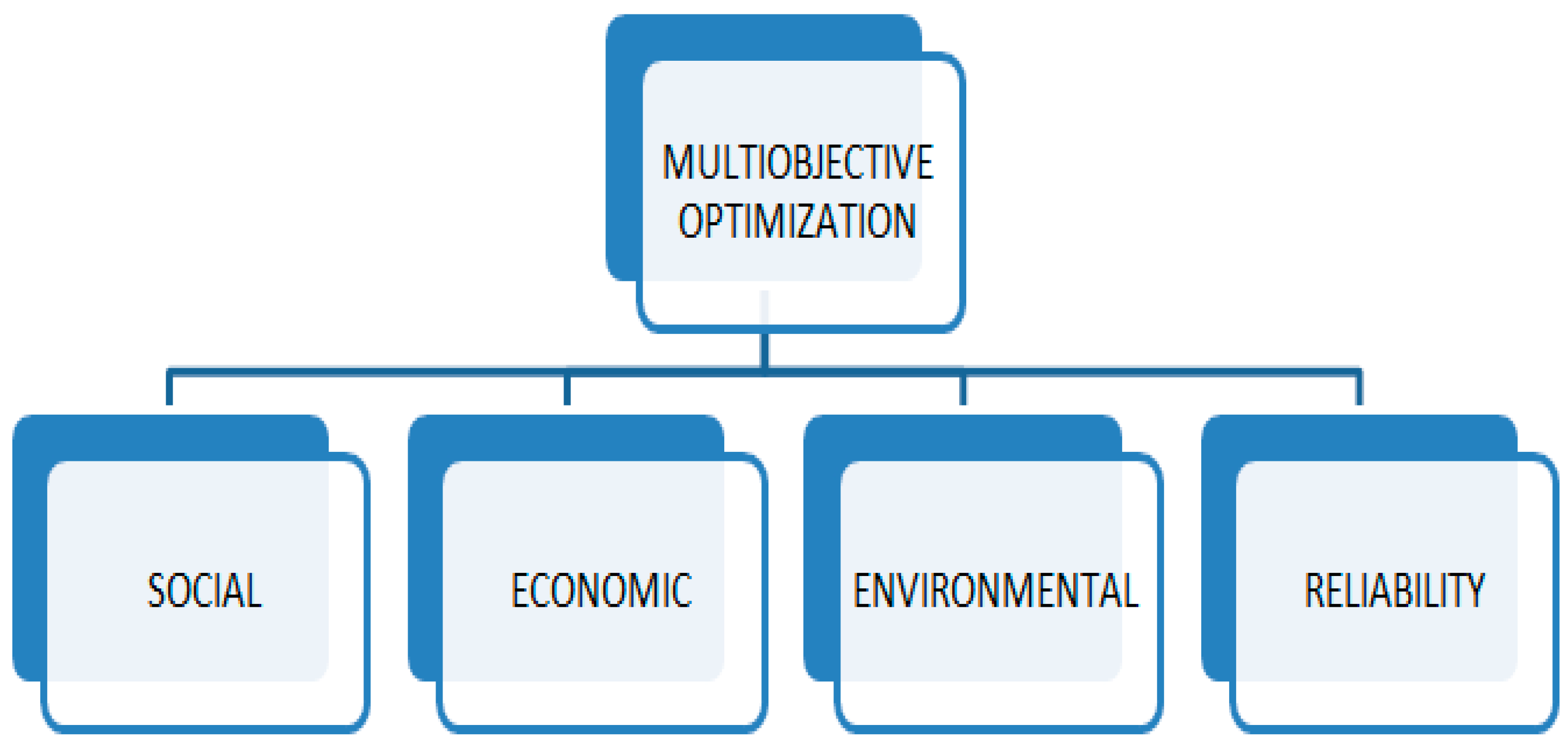
In this work, a multi-objective problem model of sustainable and reliable SCND is developed. The model pursues supply chain sustainability by taking social responsibility and green investment into account. As the third objective function, achieving customer satisfaction through reliable product delivery is the third goal, as shown by Figure 1. Based on the aforementioned notations and assumptions, the following mathematical model for multi-objective optimization can be developed.

3.2.1. Objectives

As a result, the mathematical model’s three objective functions are all of the maximization type, which is explained below:

• Goal of profitability: The primary goal function aims to increase revenue. Aggregate of the fixed, operating, transportation, and CO₂ emissions costs yields the overall costs.

$$Maximize Z_1=Profit \left(P\right)=Total Revenue\left(TR\right)-Total Cost\left(TC\right)$$

(1)

$$TR=\sum _{p\in P}[\sum _{(x,y)\in {\delta }_5}\sum _{r\in R}{C}_{er}^p{Q}_{xyr}^p+\sum _{(x,y)\in {\delta }_8}\sum _{r\in R}{C}_{br}^p{Q}_{xyr}^p+\sum _{(x,y)\in {\delta }_3}\sum _{a\in A}{C}_{ha}^p{Q}_{xya}^p]$$

(2)

$$\begin{gathered} TC=Fixed Cost\left(FC\right)+Operation Cost\left(OC\right)+Shipping Cost\left(SC\right) \\ +Disposal Cost\left(DC\right)+Emission Cost\left(EC\right) \end{gathered}$$

(3)

We can see the first objective function in Equation (1). To compute the total income, use Equation (2). Total revenue is calculated as the sum of the recycled raw materials sold to the secondary market, returned goods supplied to energy recovery facilities, and finished goods sold to the primary market.

The entire cost is computed using Equation (3).

$$\begin{array}{l}FC={\displaystyle \sum _{u\in U}}[{\displaystyle \sum _{n\in J}}{\displaystyle \sum _{g\in G}}{F}_n^{gu}{\theta }_n^{gu}+{\displaystyle \sum _{n\in K}}{F}_n^u{\theta }_n^u+{\displaystyle \sum _{n\in C}}{F}_n^u{\theta }_n^u\\ +{\displaystyle \sum _{n\in M}}{\displaystyle \sum _{l\in L}}{F}_n^{lu}{\theta }_n^{lu}]+{\displaystyle \sum _{n\in I}}{\displaystyle \sum _{a\in A}}{\displaystyle \sum _{p\in P}}{f}_{na}^p{\theta }_{na}^p+{\displaystyle \sum _{(x,y)\in \delta }}{\displaystyle \sum _{v\in V}}{\displaystyle \sum _{p\in P}}{f}_v^p{\pi }_{xy}^{vp}\end{array}$$

(4)

Equation (4) calculates fixed costs from the sum of the establishment cost of potential facilities, the supplier’s contracting cost, and the route’s reopening cost. Potential fixed costs for facility establishment are influenced by factors such as facility capacity, production technology, and raw material recycling materials [34]. Depending on the state of the market, contracts for the supply of raw materials may have different costs at different times. Using cargo trucks may have a fixed cost that varies over time.

$$\begin{array}{l}OC={\displaystyle \sum _{p\in P}}[{\displaystyle \sum _{(x,y)\in {\delta }_1}}{\displaystyle \sum _{a\in A}}{BC}_{ia}^p{Q}_{xya}^p-{\displaystyle \sum _{(x,y)\in {\delta }_2}}{\displaystyle \sum _{a\in A}}{RC}_a^p{Q}_{xya}^p+{\displaystyle \sum _{j\in J}}{\displaystyle \sum _{r\in R}}{\displaystyle \sum _{g\in G}}{PC}_{jr}^{gp}{Q}_{jr}^{gp}\\ +{\displaystyle \sum _{(x,y)\in {\delta }_5}}{\displaystyle \sum _{r\in R}}{DC}_{dr}^p{Q}_{xyr}^p\\ +{\displaystyle \sum _{d\in D}}{\displaystyle \sum _{r\in R}}{HC}_{dr}^p{I}_{dr}^p\\ +{\displaystyle \sum _{e\in E}}{\displaystyle \sum _{r\in R}}\left({EC}_{er}^p{S}_{er}^p+{OEC}_{er}^p{QN}_{er}^p\right)\\ +{\displaystyle \sum _{(x,y)\in {\delta }_5}}{\displaystyle \sum _{r\in R}}\left({CC}_{cr}^p+{OCC}_{cr}^p\right)Q_{xyr}^p+{\displaystyle \sum _{(x,y)\in {\delta }_7}}{\displaystyle \sum _{r\in R}}{\displaystyle \sum _{l\in L}}{MC}_{mr}^{lp}{Q}_{xyr}^p\\ +{\displaystyle \sum _{(x,y)\in {\delta }_9}}{\displaystyle \sum _{r\in R}}{FC}_{fr}^p{Q}_{xyr}^p]\end{array}$$

(5)

The supply chain operating costs are represented by Equation (5) and include variable costs associated with carrying out tasks in each of the facilities.

$$\begin{array}{l}SC={\displaystyle \sum _{v\in V}}{\displaystyle \sum _{p\in P}}[{\displaystyle \sum _{(x,y)\in \delta ’}}{\displaystyle \sum _{a\in A}}{D}_{xy}{\pi }_{xy}^{vp}\left((V_v^p\left({FU1}_v+{(FU2}_v{W}_a{Q}_{xya}^p\right)\right)+({\displaystyle \frac{F^p}{V_v^p}})))]\\ +[{\displaystyle \sum _{\left(x,y\right)\in {\delta }^{″}}}{\displaystyle \sum _{r\in R}}{D}_{xy}{\pi }_{xy}^{vp}((V_v^p({FU1}_V+({FU2}_V{W}_r{Q}_{xyr}^p))\\ +\left(\right(F^p)/(V_v^p\left)\right)\left)\right)]\end{array}$$

(6)

Shipment cost given by Equation (6) by adding fuel cost and vehicle use. Travel time is used to determine the cost of transportation. The distance traveled and the speed of the vehicle determine the travel time.

$$DC=\sum _{f\in F}\sum _{ p\in P}\sum _{r\in R}{w}_r^d{FC}_{fr}^p$$

(7)

Disposal cost is obtained by Equation (7), which considered the multiplication of rate of return of product r after d years of use and cost of destroying.

$$EC=\theta \left({CO}_2^{CUR}-{CO}_2^{GOV}\right)$$

(8)

$${CO}_2^{CUR}=FixedEmmission{\mathrm{C}\mathrm{O}}_2\left(\mathrm{F}\mathrm{E}\mathrm{C}\right)+\mathrm{V}\mathrm{a}\mathrm{r}\mathrm{i}\mathrm{a}\mathrm{b}\mathrm{l}\mathrm{e}\mathrm{E}\mathrm{m}\mathrm{m}\mathrm{i}\mathrm{s}\mathrm{s}\mathrm{i}\mathrm{o}\mathrm{n}{\mathrm{C}\mathrm{O}}_2\left(VEC\right)$$

(9)

$$FEC=\sum _{u\in U}[\sum _{g\in G}\sum _{j\in J}{E}_j^{gu}{\theta }_j^{gu}+\sum _{d\in D}{E}_d^u{\theta }_d^u+\sum _{c\in C}{E}_c^u{\theta }_c^u+\sum _{l\in L}\sum _{m\in M}{E}_m^{lu}{\theta }_m^{lu}]$$

(10)

$$VEC={\mu }^j\left[Energy during Operation\left(EO\right)\right]+{\mu }^l\left[Energy during Shipping\left(ES\right)\right]$$

(11)

$$\begin{array}{ll}EO={\displaystyle \sum _{r\in R}}{\displaystyle \sum _{p\in P}}[{\displaystyle \sum _{j\in J}}& {\displaystyle \sum _{g\in G}}{EP}_r^g{Q}_{jr}^{gp}+{\displaystyle \sum _{(x,y)\in {\delta }_5}}{EK}_r{Q}_{xyr}^p+{\displaystyle \sum _{(x,y)\in {\delta }_6}}{EC}_{r }{Q}_{xyr}^p\\ & +{\displaystyle \sum _{(x,y)\in {\delta }_7}}{\displaystyle \sum _{a\in A}}{\displaystyle \sum _{l\in L}}{EM}_a^l{\rho }_{ar}{Q}_{xyr}^p+{\displaystyle \sum _{(x,y)\in {\delta }_8}}{EB}_r{Q}_{xyr}^p+{\displaystyle \sum _{(x,y)\in {\delta }_9}}{EF}_r{Q}_{xyr}^p]\end{array}$$

(12)

$$\begin{gathered} ES={\sum }_{v\in V}{\sum }_{p\in P}[{\sum }_{(x,y)\in {\delta }^{\prime }}{\sum }_{a\in A}{D}_{xy}{\pi }_{xy}^{vp}({FU1}_v+({FU2}_v{W}_a{Q}_{xya}^p))]+ \\ [{\sum }_{(x,y)\in {\delta }^{″}}{\sum }_{r\in R}{D}_{xy}{\pi }_{xy}^{vp}({FU1}_v+({FU2}_v{W}_r{Q}_{xyr}^p\left)\right)] \end{gathered}$$

(13)

The supply chain’s cost of CO₂ emissions, which may surpass the government’s limit if it surpasses the permitted emission cap established by mechanisms like carbon offsets, carbon taxes or caps, and carbon cap and trade is computed by Equation (8), where θ represents penalty cost. Equation (9) demonstrates the methodology used to calculate the fixed and variable costs related to CO₂ emissions. The fixed component (CO₂ emissions from the facility establishment) is represented by Equation (10), while Equation (11) relates to the variable component (CO₂ emissions from the energy consumed). The energy used in operational procedures is computed by Equation (12), and Equation (13) computes the energy used in network shipment.

• Social responsibility objective: Social responsibility is a moral obligation for a company to take decisions that is in favor to society. We maximized the social responsibility objective using following illustrations:

$$\begin{array}{l}Corporate Social Responsibility\left(CSR\right)=Maximise Z_2\\ ={\theta }_{job}\times \left[Jobs Created\left(JC\right)\right]-{\theta }_{lpc}\times \left[Lost Days\left(LD\right)\right]\end{array}$$

(14)

$$\begin{array}{l}LD={\displaystyle \sum _{u\in U}}({\displaystyle \sum _{j\in J}}{\displaystyle \sum _{g\in G}}{lpc}_j^{gu}{\theta }_j^{gu}+{\displaystyle \sum _{d\in D}}{lpc}_d^u{\theta }_d^u+{\displaystyle \sum _{c\in C}}{lpc}_c^u{\theta }_c^u{\displaystyle \sum _{m\in M}}{\displaystyle \sum _{l\in L}}{lpc}_m^{lu}{\theta }_m^{lu})\\ +l_p\times {\displaystyle \sum _{r\in R}}{\displaystyle \sum _{u\in U}}{\displaystyle \sum _{p\in P}}({\displaystyle \sum _{j\in J}}{\displaystyle \sum _{g\in G}}{\displaystyle \frac{P_r^g{Q}_{jr}^{gp}}{{cap}_j^{gu}}}+{\displaystyle \sum _{j\in J}}{\displaystyle \sum _{d\in D}}{\displaystyle \frac{{PD}_r{Q}_{jdr}^p}{{Cap}_d^u}}\\ +{\displaystyle \sum _{e\in E}}{\displaystyle \sum _{c\in C}}{\displaystyle \frac{{PC}_r·Q_{ecr}^p}{{Cap}_c^u}}+{\displaystyle \sum _{c\in C}}{\displaystyle \sum _{m\in M}}{\displaystyle \sum _{a\in A}}{\displaystyle \sum _{l\in L}}{\displaystyle \frac{{PM}_a^l·{\rho }_{ar}·Q_{cmr}^p}{{cap}_m^{lu}}}\\ +{\displaystyle \sum _{m\in M}}{\displaystyle \sum _{k\in K}}{\displaystyle \frac{{PK}_r{Q}_{mkr}^p}{{Cap}_k^u}})\end{array}$$

(15)

$$\begin{array}{l}JC={\displaystyle \sum _{u\in U}}({\displaystyle \sum _{j\in J}}{\displaystyle \sum _{g\in G}}{\eta }_j{job}_j^{gu}{\theta }_j^{gu}+{\displaystyle \sum _{d\in D}}{\eta }_d{job}_d^u{\theta }_d^u+{\displaystyle \sum _{c\in C}}{\eta }_c{job}_c^u{\theta }_c^u\\ +{\displaystyle \sum _{m\in M}}{\displaystyle \sum _{l\in L}}{\eta }_m{job}_m^{lu}{\theta }_m^{lu}+{\displaystyle \sum _{k\in K}}{\eta }_k)\\ +jp\times {\displaystyle \sum _{r\in R}}{\displaystyle \sum _{u\in U}}{\displaystyle \sum _{p\in P}}({\displaystyle \sum _{j\in J}}{\displaystyle \sum _{g\in G}}{\displaystyle \frac{P_r^g{Q}_{jr}^{gp}}{{cap}_j^{gu}}}+{\displaystyle \sum _{j\in J}}{\displaystyle \sum _{d\in D}}{\displaystyle \frac{{PD}_r{Q}_{jdr}^p}{{cap}_d^u}}\\ +{\displaystyle \sum _{e\in E}}{\displaystyle \sum _{c\in C}}{\displaystyle \frac{{PC}_r{Q}_{ecr}^p}{{cap}_c^u}}\\ +{\displaystyle \sum _{c\in C}}{\displaystyle \sum _{m\in M}}{\displaystyle \sum _{a\in A}}{\displaystyle \sum _{l\in L}}{\displaystyle \frac{{PM}_a^l{\rho }_{ar}{Q}_{cmr}^p}{{cap}_m^{lu}}}+{\displaystyle \sum _{m\in M}}{\displaystyle \sum _{k\in K}}{\displaystyle \frac{{PK}_r{Q}_{mkr}^p}{{Cap}_k^u}})\end{array}$$

(16)

Equation (14) maximizes social responsibility in the supply chain (social responsibility is computed by deducting the number of jobs created from the number of sick leave days taken for each period). Employees’ sick leaves are computed by Equation (15), and Equation (16) computes the number of jobs created. The ultimate objective is to locate facilities in areas with higher unemployment rates and to increase job opportunities in communities of poverty.

• Environmental objective: Reducing the adverse environmental effects of supply chain operations is the main goal of environmental objectives illustrated by (*) for supply chain sustainability:

$$\begin{array}{c}Minimize{Z}_3={CO}_2^{CUR}+{\displaystyle {\sum }_{u\in U}}({\displaystyle {\sum }_{j\in J}}{\displaystyle {\sum }_{g\in G}}{\mu }^j{E}_j^{gu}+{\displaystyle {\sum }_{d\in D}}{E}_d^u+{\displaystyle {\sum }_{c\in C}}{E}_c^u+\\ {\displaystyle {\sum }_{l\in L}}{\displaystyle {\sum }_{m\in M}}{\mu }^l{E}_m^{lu}+{\displaystyle {\sum }_{k\in K}}{E}_k^u) (*)\end{array}$$

• Reliability objective: Potential suppliers and facilities have their own reliability, which, if chosen and built, adds to the supply chain’s overall fixed part reliability. The transportation and operational processes make up the supply chain’s variable part reliability.

$$R_n=P\left(T_n>p\right)=e^{-{\lambda }_{n}p}; \forall n=1,2,\dots \dots ,N$$

(17)

$$\begin{array}{ll}Maximize Z_4=& Reliability\\ & ={\lambda }_1\times \left[Contract Reliability \left(CR\right)\right]\\ & +{\lambda }_2\times \left[Facility Reliability \left(FR\right)\right]\\ & +{\lambda }_3\times \left[Operational Reliability \left(OR\right)\right]\\ & +{\lambda }_4\times \left[Shipping Reliability\left(SR\right)\right]\end{array}$$

(18)

$$CR=\sum _{i\in I}\sum _{a\in A}\sum _{p\in P}{SR}_{ia}{\theta }_{ia}^P$$

(19)

$$FR=\sum _{u\in U}[\sum _{g\in G}\sum _{n\in J}{RJ}_n^{gu}{\theta }_n^{gu}+\sum _{n\in D}{RD}_n^u{\theta }_n^u+\sum _{n\in C}{RC}_n^u{\theta }_n^u+\sum _{l\in L}\sum _{n\in M}{RM}_n^{lu}{\theta }_n^{lu}]$$

(20)

$$\begin{array}{l}OR={\displaystyle \sum _{x\in J}}{\displaystyle \sum _{r\in R}}{\displaystyle \sum _{j\in J}}{\displaystyle \sum _{p\in P}}{e}^{{-\lambda }_j^{gup }p}{TP}_r^g{Q}_{jr}^{gp}+{\displaystyle \sum _{x\in J}}{\displaystyle \sum _{y\in K}}{\displaystyle \sum _{r\in R}}{\displaystyle \sum _{p\in P}}{e}^{{-\lambda }_k^{up}p}{TK}_r{Q}_{jkr}^p\\ +{\displaystyle \sum _{x\in E}}{\displaystyle \sum _{y\in C}}{\displaystyle \sum _{r\in R}}{\displaystyle \sum _{p\in P}}{e}^{{-\lambda }_c^{up}p}{TC}_r{Q}_{ecr}^p\\ +{\displaystyle \sum _{x\in C}}{\displaystyle \sum _{y\in M}}{\displaystyle \sum _{a\in A}}{\displaystyle \sum _{r\in R}}{\displaystyle \sum _{l\in L}}{\displaystyle \sum _{p\in P}}{e}^{{-\lambda }_m^{lup}p}{TM}_a^l{\rho }_{ar}{Q}_{cmr}^p\end{array}$$

(21)

$$SR=\sum _{(x,y)\in {\delta }^{\prime }\cup {\delta }^{″}}\sum _{v\in V}\sum _{p\in P}{e}^{-({\lambda }_v+{\lambda }_{xy}·D_{xy})}{\pi }_{xy}^{vp}$$

(22)

As a result, the probability stated in Equation (17) equals the component’s reliability.

3.2.2. Constraints

By giving the classification and a brief explanation of the constraints to the given objectives, studying the model becomes easier.

• Budget constraints: One of the primary determinants of financial constraints is the amount of money a business generates. It is important to determine what would be needed to break even and recover these costs because businesses usually spend money before making it. A break-even point is attained when available revenues and expenses are equal.

$$\begin{array}{l}{\displaystyle \sum _{u\in U}}[{\displaystyle \sum _{j\in J}}{\displaystyle \sum _{g\in G}}{F}_j^{gu}{\theta }_j^{gu}+{\displaystyle \sum _{d\in D}}{F}_d^u{\theta }_d^u+{\displaystyle \sum _{c\in C}}{F}_c^u{\theta }_c^u+{\displaystyle \sum _{m\in M}}{\displaystyle \sum _{l\in L}}{F}_m^{lu}{\theta }_m^{lu}+{\displaystyle \sum _{k\in K}}{F}_k^u{\theta }_k^u]\\ \le Budget\end{array}$$

(23)

The maximum budget for a possible facility establishment is found in Equation (23).

• Carbon dioxide emission constraint: The maximum amount of carbon dioxide emissions from production operations is determined by carbon dioxide emission constraints.

$$\begin{array}{l}{CO}_2^{CUR}={\displaystyle \sum _{u\in U}}[{\displaystyle \sum _{j\in J}}{\displaystyle \sum _{g\in G}}{E}_j^{gu}{\theta }_j^{gu}+{\displaystyle \sum _{d\in D}}{E}_d^u{\theta }_d^u+{\displaystyle \sum _{c\in C}}{E}_c^u{\theta }_c^u\\ +{\displaystyle \sum _{m\in M}}{\displaystyle \sum _{l\in L}}{E}_m^{lu}{\theta }_m^{lu}+{\displaystyle \sum _{k\in K}}{E}_k^u{\theta }_k^u]+{ϵ}^j[{\displaystyle \sum _{r\in R}}{\displaystyle \sum _{p\in P}}({\displaystyle \sum _{j\in J}}{\displaystyle \sum _{g\in G}}{EP}_r^g{Q}_{jr}^{gp}\\ +{\displaystyle \sum _{\left(x,y\right)\in {\delta }_5}}{EK}_r{Q}_{xyr}^p+{\displaystyle \sum _{\left(x,y\right)\in {\delta }_6}}{EC}_r{Q}_{xyr}^p\\ +{\displaystyle \sum _{\left(x,y\right)\in {\delta }_7}}{\displaystyle \sum _{a\in A}}{\displaystyle \sum _{l\in L}}{EM}_a^l{\rho }_{ar}{Q}_{xyr}^p+{\displaystyle \sum _{\left(x,y\right)\in {\delta }_8}}{EB}_r{Q}_{xyr}^p\\ + {\displaystyle \sum _{\left(x,y\right)\in {\delta }_9}}{EF}_r{Q}_{xyr}^p)]+{ϵ}^l[{\displaystyle \sum _{v\in V}}{\displaystyle \sum _{p\in P}}({\displaystyle \sum _{\left(x,y\right)\in {\delta }^{\prime }}}{\displaystyle \sum _{a\in A}}{D}_{xy}{\pi }_{xy}^{vp}({FU1}_v\\ +\left({FU2}_v{W}_a{Q}_{xya}^p\right)))+({\displaystyle \sum _{\left(x,y\right)\in {\delta }^{″}}}{\displaystyle \sum _{r\in R}}{D}_{xy}{\pi }_{xy}^{vp}({FU1}_v\\ +\left({FU2}_v{W}_r{Q}_{xyr}^p\right)))]\end{array}$$

(24)

The amount of CO₂ in the supply chain is determined by Equation (24).

• Demand constraint: The predicted level of demand that is constrained by a number of variables, including cash flow, regulations, production capacity, and material supply, is known as constrained demand.

$$S_{er}^p={Dem}_{er}^p-\sum _{d\in D}{Q}_{der}^p, \forall e,r,p.$$

(25)

According to Equation (25), the difference between the quantity of product delivered to the market and the actual demand is what determines the lack of product in any given period.

• Facility capacity constraints: In the capacity-constrained setting, the facility can serve only a subset of the population.

$$\sum _{j\in J}{Q}_{ija}^p\ge b_{ia}{\theta }_{ia}^p \forall i,a,p$$

(26)

$$\sum _{j\in J}{Q}_{ija}^p\le {Cap}_{ia}{\theta }_{ia}^p \forall i,a,p$$

(27)

$$\sum _{r\in R}{P}_r^g{Q}_{jr}^{gp}\le \sum _{u\in U}{Cap}_j^{gu}{\theta }_j^{gu} \forall g,p$$

(28)

$$\sum _{r\in R}\sum _{e\in E}{PD}_r{Q}_{der}^p\le \sum _{u\in U}{Cap}_d^u{\theta }_d^u \forall d,p$$

(29)

$$\sum _{r\in R}{v}_r{I}_{dr}^p\le \sum _{u\in U}{VCap}_d^u{\theta }_d^u \forall d,p$$

(30)

$$\sum _{c\in C}{Q}_{cbr}^p\le {Cap}_{br} \forall b,r,p$$

(31)

$$\sum _{c\in C}{Q}_{cfr}^p\le {Cap}_{fr} \forall f,r,p$$

(32)

$$\sum _{l\in L}{PM}_a^l{\rho }_{ar}{Q}_{cmr}^p\le \sum _{l\in L}\sum _{u\in U}{Cap}_m^{lu}{\theta }_m^{lu} \forall m,p$$

(33)

$$\sum _{e\in E}\sum _{r\in R}{PC}_r{Q}_{ecr}^p\le \sum _{u\in U}{Cap}_c^u{\theta }_c^u \forall c,p$$

(34)

The minimum and maximum supplier capacities are displayed by Equations (26) and (27), respectively. Equation (28) shows the manufacturing center’s maximum capacity. The maximum distribution capacity and warehouse capacity of the distribution center are shown in Equations (29) and (30), respectively. The maximum capacity of the energy recovery center is given by Equation (31), and Equation (32) displays the maximum capacity of the landfill center. The maximum collection capacity of collection centers is represented by Equation (33). Equation (34) describes the recycling center’s maximum raw material recycling capacity.

• Allocation constraint: Allocation constraints can be defined to control behavior such as the following:

$$\sum _{g\in G}\sum _{u\in U}{\theta }_j^{gu}\le 1 \forall p$$

(35)

$$\sum _{u\in U}{\theta }_d^u\le 1 \forall d$$

(36)

$$\sum _{u\in U}{\theta }_c^u\le 1 \forall c$$

(37)

$$\sum _{l\in L}\sum _{u\in U}{\theta }_m^{lu}\le 1 \forall m$$

(38)

Each manufacturing center, distribution center, collection center, and recycling center, if established, may only have one capacity level, according to Equations (35)–(38).

• Constraint on flow balance: The conditional minimum flow establishes that in order to use this source site–destination site combination for any shipments, a minimum flow is necessary.

$$\sum _{g\in G}{Q}_{jr}^{gp}=\sum _{k\in K}{Q}_{jkr}^p \forall j, r, p$$

(39)

$$\sum _{i\in I}{Q}_{ija}^p+\sum _{m\in M}{Q}_{mja}^p=\sum _{r\in R}\sum _{g\in G}{q}_{ar}{Q}_{jr}^{gp} \forall j,a,p$$

(40)

$$I_{dr}^p=I_{dr}^{p-1}+\sum _{j\in J}{Q}_{jdr}^p-\sum _{e\in E}{Q}_{der}^p \forall d, r$$

(41)

$$\sum _{e\in E}\sum _{p=t}^{min(p+D_r-1,p)}{Q}_{der}^p-\sum _{j\in J}\sum _{p\in P}{Q}_{jdr}^p\ge 0 \forall d,r,p\&p\ne P$$

(42)

$$\sum _{j\in J}{Q}_{mja}^p=\sum _{r\in R}\sum _{c\in C}{\rho }_{ar}{\sigma }_a{Q}_{cmr}^p \forall m, a, p$$

(43)

$$\sum _{h\in H}{Q}_{mha}^p=\sum _{r\in R}\sum _{c\in C}{\rho }_{ar}\left(1-{\sigma }_a\right)Q_{cmr}^p \forall m, a, p$$

(44)

$${QR}_{er}^p=\sum _{d=0}^{D_r}{\omega }_r^d\left({Dem}_{er}^{p-d}-S_{er}^{p-d}\right) \forall e, r, p, \ge D_r$$

(45)

$${QR}_{er}^p=0 \forall e, r, p, p<D_r$$

(46)

$$I_{kr}^p=0 \forall r, k,p=1$$

(47)

$$\sum _{c\in C}{Q}_{ecr}^p\le {QR}_{er}^p \forall e, r, p$$

(48)

$${QN}_{er}^p={QR}_{er}^p-\sum _{c\in C}{Q}_{ecr}^p \forall e,r,p$$

(49)

$$\sum _{b\in B}{Q}_{cbr}^p=\sum _{e\in E}{\beta }_r{Q}_{ecr}^p \forall c,r,p$$

(50)

$$\sum _{e\in E}{\gamma }_r{Q}_{ecr}^p=\sum _{m\in M}{Q}_{cmr}^p \forall c,r,p$$

(51)

$$\sum _{e\in E}{Q}_{ecr}^p=\sum _{f\in F}{Q}_{cfr}^p+\sum _{m\in M}{Q}_{cmr}^p+\sum _{b\in B}{Q}_{cbr}^p \forall c,r,p$$

(52)

Equation (39) does not allow for storage for the final products. Manufacturing centers can obtain the raw materials they need by purchasing from suppliers or recycling centers as shown by Equation (40). The maintenance quantity of final products in the distribution center is displayed by Equation (41). Equation (42) shows that the inventory of final products at the beginning of the first planning period is zero. The percentage of recycled raw materials shared by the secondary market and the manufacturer is represented by Equations (43) and (44), respectively. The amount of time used determines the end-of-life product (uptrend) return rate, according to Equation (45). Equation (46) demonstrates that finished goods do not reappear before their useful lives are up. According to Equation (47), the maximum amount of time that finished goods can be stored in a warehouse is one period less than when their life ends. Not every product that is returned from the primary market may be collected by the reverse chain, as demonstrated by Equation (48). The uncollected returned products are shown in Equation (49). Three centers are identified by Equations (50)–(52) for the collected end-of-life products: energy recovery, recycling, and landfill.

• Shipping capacity constraints: Shipping capacity constraints are the limitations that arise across the shipping arms of the supply chain.

$$\sum _{a\in A}{v}_a{Q}_{xya}^p\le {vcap}^v{\pi }_{xy}^{vp} \forall \left(x,y\right)\in {\delta }^{\prime }, v, p$$

(53)

$$\sum _{r\in R}{v}_r{Q}_{xyr}^p\le {vcap}^v{\pi }_{xy}^{vp} \forall \left(x,y\right)\in {\delta }^{″}, v, p$$

(54)

$$\sum _{a\in A}{w}_a{Q}_{xya}^p\le {wcap}^v{\pi }_{xy}^{vp} \forall \left(x,y\right)\in {\delta }^{\prime }, v, p$$

(55)

$$\sum _{r\in R}{w}_r{Q}_{xyr}^p\le {wcap}^v{\pi }_{xy}^{vp} \forall \left(x,y\right)\in {\delta }^{″}, v, p$$

(56)

Vehicle volume is represented by Equations (53) and (54), and vehicle weight capacity is represented by Equations (55) and (56).

• Rational constraints: A logical constraint combines linear constraints by means of logical operators, such as

$${\theta }_{ia}^p,{\theta }_j^{gu},{\theta }_d^u,{\theta }_c^u,{\theta }_m^{lu},{\pi }_{xy}^{vp}\in \left\{\mathrm{0,1}\right\},$$

(57)

$$Q_{xya}^{vp},Q_{xyr}^{vp},Q_{jr}^{gp},I_{dr}^p,{QR}_{xr}^p,{QN}_{er}^p,S_{er}^p,{CO}_2^{CUR}\ge 0$$

(58)

Logical constraints for discrete and continuous decision variables are given by Equations (57) and (58).

3.3. Model’s Linearization

We introduce two decision variables in order to convert a non-linear model into a linear model. Two new choice variables were thus constructed in order to linearize the model and remove the non-linear elements. Equations (6) and (13) pertain to the first objective function, and Equation (23) pertains to the CO₂ emissions constraint, which causes multiplication relations between binary and positive variables, which cause the model to become non-linear. After linearization of the model, the WSM and TOPSIS methods were used to find the optimal solution.

For the decision variables,

Table 2. Decision variables after linearization of model.

Symbol	Description
${\mathit{S}\mathit{S}}_{\mathit{x}\mathit{y}\mathit{a}}^{\mathit{v}\mathit{p}}$	$\mathrm{The} \mathrm{quantity} \mathrm{of} \mathrm{raw} \mathrm{materials} \mathrm{that} \mathrm{a} \mathrm{vehicle} \mathrm{v} \mathrm{transports} \mathrm{between} \mathrm{locations} \left(\mathit{x},\mathit{y}\right)\in {\mathit{\delta }}^{\prime }$ during time p
${\mathit{S}\mathit{S}}_{\mathit{x}\mathit{y}\mathit{r}}^{\mathit{v}\mathit{p}}$	$\mathrm{Throughout} \mathrm{time} \mathrm{p}, \mathrm{the} \mathrm{quantity} \mathrm{of} \mathrm{product} \mathrm{r} \mathrm{moved} \mathrm{by} \mathrm{vehicle} \mathrm{v} \mathrm{between} \mathrm{facilities} \left(\mathit{x},\mathit{y}\right)\in {\mathit{\delta }}^{″}$

provides a definition of the symbols. Equation (6) becomes Equation (59) after linearization, and Equations (13) and (23) become Equation (60). Equation (67) imposes constraints on the newly introduced decision variables.

$$\begin{array}{l}SC={\displaystyle \sum _{p\in P}}{\displaystyle \sum _{v\in V}}[{\displaystyle \sum _{\left(x,y\right)\in {\delta }^{\prime }}}{\displaystyle \sum _{a\in A}}{FU1}_v{V}_v^p{D}_{xy}{\pi }_{xy}^{vp}+{FU2}_v{V}_v^p{W}_a{D}_{xy}{SS}_{xya}^{vp}+{\displaystyle \frac{F_d^p{D}_{xy}{\pi }_{xy}^{vp}}{V^v}}]\\ +[{\displaystyle \sum _{\left(x,y\right)\in {\delta }^{″}}}{\displaystyle \sum _{r\in R}}{FU1}_v{V}_v^p{D}_{xy}{\pi }_{xy}^{vp}+{FU2}_v{V}_v^p{W}_r{D}_{xy}{SS}_{xyr}^{vp}\\ +{\displaystyle \frac{F_d^p{D}_{xy}{\pi }_{xy}^{vp}}{V^v}}]\end{array}$$

(59)

$$\begin{array}{c}CES={\displaystyle \sum _{p\in P}}{\displaystyle \sum _{v\in V}}[{\displaystyle \sum _{(x,y)\in {\delta }^{\prime }}}{\displaystyle \sum _{a\in A}}{FU1}_v{D}_{xy}{\pi }_{xy}^{vp}+{FU2}_v{W}_a{D}_{xy}{SS}_{xya}^{vp}]\\ +\left[{\displaystyle \sum _{\left(x,y\right)\in {\delta }^{″}}}{\displaystyle \sum _{r\in R}}{FU1}_v{D}_{xy}{\pi }_{xy}^{vp}+{FU2}_v{W}_r{D}_{xy}{SS}_{xyr}^{vp}\right]\end{array}$$

(60)

$${SS}_{xya}^{vp}\le Q_{xya}^p \forall \left(x,y\right)\in {\delta }^{\prime },a,v,$$

(61)

$${SS}_{xya}^{vp}\le BM{\pi }_{xy}^{vp} \forall \left(x,y\right)\in {\delta }^{’},v,a,p$$

(62)

$${SS}_{xya}^{vp}\ge Q_{xya}^p-BM\left(1-{\pi }_{xy}^{vp}\right) \forall \left(x,y\right)\in {\delta }^{\prime },v,a,p$$

(63)

$${SS}_{xyr}^{vp}\le Q_{xyr}^p \forall \left(x,y\right)\in {\delta }^{″}, v, r, p$$

(64)

$${SS}_{xyr}^{vp}\le BM{\pi }_{xy}^{vp} \forall \left(x,y\right)\in {\delta }^{″}, v, r, p$$

(65)

$${SS}_{xyr}^{vp}\ge Q_{xyr}^p-BM\left(1-{\pi }_{xy}^{vp}\right) \forall \left(x,y\right)\in {\delta }^{″}, v, r, p$$

(66)

$${SS}_{xya}^{vp}\ge {SS}_{xyr}^{vp}$$

(67)

$${SS}_{xya}^{vp},{SS}_{xyr}^{vp}\ge 0$$

(68)

Equation (6) becomes Equation (59) after linearization, and Equations (13) and (23) become Equation (60). Equation (68) imposes constraints on the newly introduced decision variables.

3.4. Model Decisions

Two different methods, WSM and TOPSIS, are used to solve the supplier selection problem and are discussed below.

3.4.1. Weighted Sum Approach

A straightforward and popular method for multi-criteria decision-making (MCDM) is the weighted sum method (WSM). It assists in prioritizing options based on a number of factors by giving each criterion a weight based on its significance.

In multi-objective optimization (MOO), the weighted sum approach is still commonly utilized in spite of its limitations in terms of parsing the Pareto optimal set. It accomplishes this by regularly changing the weights and by producing a single solution point that represents preferences that were likely taken into account when choosing a single set of weights [35]. The linear scale transformation method is used for normalization of the decision matrix. For benefit attributes ${\displaystyle \frac{{\mathit{x}}_{\mathit{i}\mathit{j}}}{\sum {\mathit{x}}_{\mathit{i}\mathit{j}}}}$ and for cost attribute ${\displaystyle \frac{\frac{1}{{\mathit{x}}_{\mathit{i}\mathit{j}}}}{\sum \frac{1}{{\mathit{x}}_{\mathit{i}\mathit{j}}}}}$, the weighted sum approach combines all of the multi-objective functions into a single scalar composite objective function.

$$F\left(x\right)=w_1{f}_1\left(x\right)+w_2{f}_2\left(x\right)+\dots +w_m{f}_m\left(x\right)$$

(69)

The weighting coefficients, $w=\left(w_1,w_2,\dots ,w_m\right)$ must be assigned with care because the solution heavily relies on the selection of these coefficients. It is evident that these weights must be positive and satisfying.

$$\sum _{i=1}^m{w}_i=1, w_i\in \left(\mathrm{0,1}\right)$$

(70)

3.4.2. Technique for Order of Preference by Similarity to Ideal Solution Method

According to their geometric distance from an ideal solution and a negative ideal solution, alternatives are assessed using the technique for order preference by similarity to ideal solution (TOPSIS). Suitable for a variety of applications, TOPSIS is a useful tool for multi-criteria decision-making that strikes a compromise between ease of use and efficacy.

TOPSIS is regarded as an efficient MCDM method because of its unique properties, which combine high consistency and low computational effort. This method essentially yields a single performance response value by combining the multi-response values.

Conversely, a theoretical strategy called the “negative ideal solution” would result in higher costs for the requirements or features and lower benefits. The optimal choice, which also serves as the problem’s solution, is the one that is most similar to the ideal, positive solution and most dissimilar from the ideal, negative solution. It is defined by the Euclidean/geometric distance, the ideal solution, and the negative ideal.

This analysis is guided by the database’s maximum and minimum values. Trade-offs between the criteria are possible with this method’s more realistic modeling form, which permits one to overlook a subpar result when evaluating one criterion in favor of a subpar result when evaluating another. The following m × n decision matrix, consisting of p alternatives and q criteria, is considered in all MCDM problems:

$$X={\left[\begin{array}{ccc}{x}_{11}& \cdots & x_{1q}\\ ⋮& \ddots & ⋮\\ x_{p1}& \cdots & x_{pq}\end{array}\right]}_{p\times q}$$

$\mathrm{i}=1,2,\dots ,\mathrm{p}$ and $\mathrm{j}=1,2,\dots ,\mathrm{a}\mathrm{n}\mathrm{d}\mathrm{q}$ are the values of all the equations in this section. There are six primary steps in the TOPSIS’s selection of the best alternative:

• Step 1: The decision matrix’s normalization

In every MCDM problem, there are various types of criteria with various units. These criteria must be dimensionless (without units) in order to be compared and the normalization process makes this feasible. For this, a variety of techniques can be applied. For instance, using the vector normalization technique, normalized values for each ${\mathrm{x}}_{\mathrm{i}\mathrm{j}}$ in the decision matrix are displayed as

$$r_{ij}={\displaystyle \frac{x_{ij}}{\sqrt{{\sum }_{i=1}^p{x}_{ij}^2}}}$$

(71)

• Step 2: The weighted normalized matrix calculation

One can compute the weighted normalized decision matrix $\left(\mathit{U}\right)$ as

$$U={\left(u_{ij}\right)}_{q\times p}$$

(72)

where$, u_{ij}=w_j{r}_{ij}.$

• Step 3: Finding the ideal solutions, both positive and negative

To find both positive and negative ideal solutions, it is advised to use the following equations:

$$B^{*}=\left\{v_1^{*},v_2^{*},\dots ,v_q^{*}\right\}=\left\{\left(\underset{j}{\max }{v}_{ij}|i\in I^{\prime }\right),\left(\underset{j}{\min }{v}_{ij}|i\in I^{″}\right)\right\}$$

(73)

$$B^{-}=\left\{v_1^{-},v_2^{-},\dots ,v_q^{-}\right\}=\left\{\left(\underset{j}{\min }{v}_{ij}|i\in I^{\prime }\right),\left(\underset{j}{\max }{v}_{ij}|i\in I^{″}\right)\right\}$$

(74)

According to these equations, $B^{*}$ is obtained by aggregating the best performance of$U$, and $B^{-}$ is derived from the normalized matrix’s worst performances.

• Step 4: Separation measures calculation

This step involves calculating the distance between alternatives with $B^{*}$ and $B^{-}$ after positive and negative solutions has been determined. There are several ways to calculate distances, of which the classical Euclidean distance is one of the more popular:

$$D_i^{\mathrm{*}}=\sqrt{\sum _{j=1}^q{\left(v_{ij}-v_j^{*}\right)}^2}$$

(75)

$$D_i^{-}=\sqrt{\sum _{j=1}^q{\left(v_{ij}-v_j^{-}\right)}^2}$$

(76)

• Step 5: Determining the relative closeness

The following equation is used to calculate the relative closeness factor, which has a range of 0 to 1.

$$C_i^{*}={\displaystyle \frac{D_i^{-}}{D_i^{+}+D_i^{-}}}$$

(77)

• Step 6: Ranking of suppliers

In the TOPSIS final step, the options are ranked from best, with the biggest $C_i^{*}$ (i.e., the $C_i^{*}$ value closest to 1), to the worst, with the lowest $C_i^{*}$ value. The solution is the alternative which is ranked highest on the list and has the largest $C_i^{*}$ value.

In the ultimate phase of TOPSIS, the choices are arranged in order of best to worst, with the highest $C_i^{*}$ value. The first option on the list with the largest $C_i^{*}$ (i.e., the $C_i^{*}$ value closest to 1) value is the solution.

4. Results and Discussions

The mathematical model covered in the previous section is solved numerically in this section. Four suppliers with three criteria make up the numerical example. To ascertain whether criteria conflict with one another, an outcome matrix is made, as shown in

Table 3. Decision matrix for supplier selection.

Alternatives	Criteria
	Reliability (0.4)	Fuel-Efficiency (km/lt.) (0.3)	Cost (in lakhs) (0.3)
A1	9	9	8
A2	7	8	7
A3	6	8	9
A4	7	8	6

. The alternative’s value for A1, A2, A3, and A4 has been assumed as 9, 7, 6, and 7 for reliability; 9, 8, 8, and 8 for fuel efficiency; and 8, 7, 9, and 6 for costs. Consequently, this SCND problem requires multi-objective optimization since single-objective optimization is unable to produce a satisfactory compromise between competing objective functions.

This paper considers a mathematical model with three objectives: profit, social responsibility, and reliability. These objectives may be incompatible with one another. As a result, the decision-maker has to trade off between each goal and consider its advantages.

Multi-objective problem-solving techniques were used to solve the suggested sustainable and reliable SCND problem (relationships one to sixty-six), and the results were compared with WSM and TOPSIS methods. The normalized form of these findings is shown for the sample in

Table 4. Normalization of decision matrix.

Supplier	Technique	Normalized Decision Matrix			${\mathit{F}}_{\mathit{x}}$
		${\mathit{C}}_1$	${\mathit{C}}_2$	${\mathit{C}}_3$	${\mathit{C}}_{\mathit{i}}^{\mathit{*}}$
First	WSM	0.31	0.27	0.23	0.74
	TOPSIS	0.61	0.54	0.53	0.38
Second	WSM	0.24	0.24	0.26	0.246
	TOPSIS	0.48	0.48	0.46	0.804
Third	WSM	0.21	0.24	0.02	0.216
	TOPSIS	0.41	0.48	0.59	0.67
Fourth	WSM	0.24	0.24	0.31	0.261
	TOPSIS	0.48	0.48	0.4	0.889

. One significant benefit that makes the WSM easier to use in solving the multi-objective problem in SCND is its faster computing time.

First, the WSM technique is utilized in order to compute the rank. Second, the alternatives are ranked using the generalized TOPSIS.

Table 5. Ranking of Suppliers.

Alternative	TOPSIS	WSM
A1	4	1
A2	2	3
A3	3	4
A4	1	2

displays the results of these computations, which rank each alternative according to each criterion.

We consider an individual decision-maker for the selection of an ideal supplier. For example, we have four alternatives (supplier), and we need to choose the ideal one. The normalized decision matrix is obtained by using the linear scale transformation method. The global score (preference score) is calculated by using Equation (67). Using the AHP method, we calculate the weights of criteria. Weights are determined for each criterion by combining the outcomes of the pair-wise comparisons.

To ensure that the derived results were accurate, a sensitivity analysis was performed. Sensitivity analysis is used to track changes in ranking where, one primary attribute is given the maximum weight while the others are given the lowest weight [36]. To this aim, three criteria were taken into account. For instance, sub-criterion C1’s weight is assumed to be 0.4, which is the maximum value, and the weights of the other two sub-criteria are 0.3, which is the minimum value. This procedure was then carried out for all two sub-criteria. The TOPSIS was then used for ranking. The outcome demonstrates that, in every circumstance, supplier 4 is the best option. We developed a sustainable and reliable supply chain network design model. Further, we tried to verify the above model using two multi-criteria decision-making methods, i.e., the WSM and TOPSIS methods. We considered reliability as a criterion in our case study, along with cost and fuel efficiency. The outcomes from the WSM and TOPSIS methods are compared and ranked. The proposed developed model is an improvement on the existing sustainable supply chain network design as it deals with reliability criterion as well as the reliability of the supply of manufactured products as an objective. The proposed model is a multi-objective linear programming (MOLP) model. In order to optimize the MOLP problem, multi-objective decision-making methods are required, such as the epsilon-constraint method and the weighted sum method. A multi-criteria decision-making (MCDM) technique called TOPSIS (technique for order of preference by similarity to ideal solution) has been used in the past for research and decision-making. It ranks alternatives by optimizing input parameters to obtain the maximum overall output from the system. Recently, search techniques and mathematical principles of nature-inspired algorithms have been created for optimization issues [37]. In order to achieve the objectives of competitive supply chains (SCs), this study intends to investigate the background, justifications, and specific benefits of applying TOPSIS in the field of materials science and engineering. In comparison to other MCDM methods that are comparatively more complex and time-consuming, the outcomes of TOPSIS have performed exceptionally well. Engineers, practitioners, academicians, researchers, and SC managers will benefit from this study’s application of TOPSIS for output optimization in a variety of fields.

The weighted sum method (WSM) is widely used in decision-making because it is easy to evaluate several choices that produce consistent outcomes. Comparative weights are assigned to each criterion in the WSM’s criteria development process by assessing the relevance of the workstation requirements in the given situation.

This study looked into supply chain reliability in a two-stage stochastic programming model to create dependable forward/backward, closed-loop, green, four-echelon supply chain networks. Remanufacturing is the novel concept in this suggested supply chain model. Remanufacturing significantly decreases the amount of waste sent to landfills by reprocessing materials and extending product lifecycles, promoting a circular economy. Recycling and remanufacturing reduces the need for new materials by reusing and recycling existing products, conserving natural resources and minimizing the environmental impact. Lower production costs can be achieved through the use of recycled materials and reduced raw material procurement, leading to improved profit margins. A closed-loop supply chain (CLSC) incorporates processes that enable products to be returned, recycled, and remanufactured, creating a sustainable cycle. It streamlines processes by integrating recycling and remanufacturing into the supply chain, which can lead to faster turnaround times and reduced inventory costs. By implementing a closed-loop supply chain with recycling and remanufacturing, organizations can achieve both economic and environmental benefits, contributing to a more sustainable future while maintaining a competitive advantage.

The goal of this model was to optimize the supply chain’s overall reliability by using the theory of structural reliability. Additionally, our suggested model reduced supply chain expenses by the definition of recycling facilities, the price of enforcing illegal carbon emissions, and harms. The locations of factories, warehouses, and recycling centers were optimized by the model taking into account the flow between the stochastic modes for carbon price and demand in various industries and the best arrangements.

Adjusting the objective weights at different points in proportion to the total objective weights in each set that equals 1 is how sensitivity analysis for the aforementioned model is performed. To ascertain the effect of objective weights on the order allocation problem, sensitivity analysis is utilized.

5. Conclusions

The goal of the supply chain optimization problem presented in this paper is to build multimodal, dependable, and sustainable supply chains. This proposed supply chain model’s innovative idea is remanufacturing. By reprocessing materials and prolonging product lifecycles, remanufacturing promotes a circular economy and drastically reduces the quantity of waste that is dumped in landfills, thereby reducing the influence on the environment, conserving natural resources, and eliminating the need for new materials by recycling and reusing current products. Reduced raw material procurement and the utilization of recycled resources can lower production costs and increase profit margins. The mechanisms that allow products to be returned, recycled, and remanufactured are part of a closed-loop supply chain (CLSC), which creates a sustainable cycle and reduces inventory costs and turnaround times by streamlining procedures through the supply chain’s integration of recycling and remanufacturing.

This study suggests a novel method that uses multi-criteria decision analysis and symmetry/asymmetry supply chain data in order to optimize sustainable supplier selection as part of the supply chain network design. A mixed-integer linear programming model is developed to resolve conflicts between criteria, with reliability serving as the main goal and sustainability dimensions serving as constraints. The model that is being presented makes multiple contributions to the literature. Initially, the proposed model ensures a specific degree of overall reliability. Second, the literature incorporates multimodality, sustainability with facility and shipping capacity constraints, and reliability for the first time. The model also accounts for carbon emissions from transportation and production processes. Decision-makers can select the most profitable and reliable suppliers for their supply operations by using the study’s findings. The proposed strategy is applied to numerical data and verified as well. It is observed that the developed approach is more efficient than the existing supply chain design. Two methods, WSM and TOPSIS, are utilized in this multi-objective problem, and a numerical example with four different suppliers is illustrated. The criteria weights are obtained using the analytical hierarchy process. The outcomes of the TOPSIS and WSM techniques were contrasted.

However, there are some issues that need to be addressed in further studies. Evaluating network reliability is a worthwhile study, and selecting the appropriate closeness coefficient in real-world scenarios is a challenging and practical issue. Multiple suppliers and products (materials) are frequently found in supply chains. Network reliability assessment may also consider other factors, such as manufacturer production technologies, the use of renewable energy sources, and carbon emissions during transportation, in order to improve sustainability in the supply chain. There is a lack of literature on the optimization of supply chain networks with multistate delivery capacity and supplier sustainability from the perspective of network reliability. One avenue for future research could be the development of an appropriate network model that addresses this optimization problem with network reliability. Future research could use other multi-criteria decision-making methods to solve the same problem.

References

1. Xia, Y.; Tang, T.L.-P. Sustainability in supply chain management: Suggestions for the auto industry. Manag. Decis. 2011, 49, 495–512. [Google Scholar] [CrossRef]
2. Zailani, S.; Jeyaraman, K.; Vengadasan, G.; Premkumar, R. Sustainable supply chain management (SSCM) in Malaysia: A survey. Int. J. Prod. Econ. 2012, 140, 330–340. [Google Scholar] [CrossRef]
3. Eltayeb, T.; Zailani, S. Going green through green supply chain initiatives toward environmental sustainability. Oper. Supply Chain Manag. Int. J. 2014, 2, 93–110. [Google Scholar] [CrossRef]
4. Gualandris, J.; Klassen, R.D.; Vachon, S.; Kalchschmidt, M. Sustainable evaluation and verification in supply chains: Aligning and leveraging accountability to stakeholders. J. Oper. Manag. 2015, 38, 1–13. [Google Scholar] [CrossRef]
5. Lin, Y.H.; Tseng, M.L. Assessing the competitive priorities within sustainable supply chain management under uncertainty. J. Clean. Prod. 2016, 112, 2133–2144. [Google Scholar] [CrossRef]
6. Zhang, S.; Lee, C.K.M.; Wu, K.; Choy, K.L. Multi-objective optimization for sustainable supply chain network design considering multiple distribution channels. Expert Syst. Appl. 2016, 65, 87–99. [Google Scholar] [CrossRef]
7. Fallahpour, A.; Olugu, E.U.; Musa, S.N.; Wong, K.Y.; Noori, S. A decision support model for sustainable supplier selection in sustainable supply chain management. Comput. Ind. Eng. 2017, 105, 391–410. [Google Scholar] [CrossRef]
8. Valinejad, F.; Rahmani, D. Sustainability risk management in the supply chain of telecommunication companies: A case study. J. Clean. Prod. 2018, 203, 53–67. [Google Scholar] [CrossRef]
9. Gholami, F.; Paydar, M.M.; Hajiaghaei-Keshteli, M.; Cheraghalipour, A. A multi-objective robust supply chain design considering reliability. J. Ind. Prod. Eng. 2019, 36, 385–400. [Google Scholar] [CrossRef]
10. Asim, Z.; Jalil, S.A.; Javaid, S. An uncertain model for integrated production-transportation closed-loop supply chain network with cost reliability. Sustain. Prod. Consum. 2019, 17, 298–310. [Google Scholar] [CrossRef]
11. Daehy, Y.; Krishnan, K.; Alsaadi, A.; Alghamdi, S. Effective cost minimization strategy and an optimization model of a reliable global supply chain system. Uncertain Supply Chain Manag. 2019, 7, 381–398. [Google Scholar] [CrossRef]
12. Tseng, M.L.; Wu, K.J.; Lim, M.K.; Wong, W.P. Data-driven sustainable supply chain management performance: A hierarchical structure assessment under uncertainties. J. Clean. Prod. 2019, 227, 760–771. [Google Scholar] [CrossRef]
13. Fazli-Khalaf, M.; Naderi, B.; Mohammadi, M.; Pishvaee, M.S. Design of a sustainable and reliable hydrogen supply chain network under mixed uncertainties: A case study. Int. J. Hydrogen Energy 2020, 45, 34503–34531. [Google Scholar] [CrossRef]
14. Kabadurmus, O.; Erdogan, M.S. Sustainable, multimodal and reliable supply chain design. Ann. Oper. Res. 2020, 292, 47–70. [Google Scholar] [CrossRef]
15. Farooq, M.U.; Saqlain, M. The selection of LASER as surgical instrument in medical using neutrosophic soft set with generalized fuzzy TOPSIS, WSM and WPM along with MATLAB coding. Neutrosophic Sets Syst. 2021, 40, 3. [Google Scholar]
16. Hazrati, R.; Samaei, M.; Hejri, F.M.; Haddad, S.; Amiriyan, S. Designing a Medical Supply Chain Network Considering the Risk of Supply and Flexible Production in Two-Stage Uncertain Conditions. Math. Probl. Eng. 2022, 2022, 5762185. [Google Scholar] [CrossRef]
17. Madanchian, M.; Taherdoost, H. A comprehensive guide to the TOPSIS method for multi-criteria decision making. Sustain. Soc. Dev. 2023, 1, 2220. [Google Scholar] [CrossRef]
18. Ismail, M.M.; Ahmed, Z.; Abdel-Gawad, A.F.; Mohamed, M. Toward Supply Chain 5.0: An Integrated Multi-Criteria Decision-Making Models for Sustainable and Resilience Enterprise. Decis. Mak. Appl. Manag. Eng. 2024, 7, 160–186. [Google Scholar] [CrossRef]
19. Singh, S.; Agrawal, V.; SAXENA, K.K.; Mohammed, K.A. Optimization on Manufacturing Processes at Indian Industries Using TOPSIS. Indian J. Eng. Mater. Sci. (IJEMS) 2023, 30, 32–44. [Google Scholar]
20. Abhilasha, A.; Danish, F. Optimization for a sustainable supply chain using Fuzzy VIKOR method: An application on a real dataset. IEEE Access 2024, 12, 131882–131891. [Google Scholar] [CrossRef]
21. Nosrati, M.; Khamseh, A. Reliability optimization in a four-echelon green closed-loop supply chain network considering stochastic demand and carbon price. Uncertain Supply Chain Manag. 2020, 8, 457–472. [Google Scholar] [CrossRef]
22. Tirkolaee, E.B.; Mardani, A.; Dashtian, Z.; Soltani, M.; Weber, G.W. A novel hybrid method using fuzzy decision making and multi-objective programming for sustainable-reliable supplier selection in two-echelon supply chain design. J. Clean. Prod. 2020, 250, 119517. [Google Scholar] [CrossRef]
23. Ahmadini, A.A.H.; Modibbo, U.M.; Shaikh, A.A.; Ali, I. Multi-objective optimization modelling of sustainable green supply chain in inventory and production management. Alex. Eng. J. 2021, 60, 5129–5146. [Google Scholar] [CrossRef]
24. Acquah, I.S.K.; Naude, M.J.; Sendra-García, J. Supply chain collaboration in the petroleum sector of an emerging economy: Comparing results from symmetrical and asymmetrical approaches. Technol. Forecast. Soc. Change 2021, 166, 120568. [Google Scholar] [CrossRef]
25. Salehi, S.; Mehrjerdi, Y.Z.; Sadegheih, A.; Hosseini-Nasab, H. Designing a resilient and sustainable biomass supply chain network through the optimization approach under uncertainty and the disruption. J. Clean. Prod. 2022, 359, 131741. [Google Scholar] [CrossRef]
26. Eslamipoor, R.; Nobari, A. A reliable and sustainable design of supply chain in healthcare under uncertainty regarding environmental impacts. J. Appl. Res. Ind. Eng. 2023, 10, 256–272. [Google Scholar]
27. Mirzagoltabar, H.; Shirazi, B.; Mahdavi, I.; Arshadi Khamseh, A. Integration of sustainable closed-loop supply chain with reliability and possibility of new product development: A robust fuzzy optimisation model. Int. J. Syst. Sci. Oper. Logist. 2023, 10, 2119112. [Google Scholar] [CrossRef]
28. Lin, K.Y.; Lin, Y.K. Sustainable supply chain evaluation with supplier sustainability in terms of reliability. Ann. Oper. Res. 2024, 1–17. [Google Scholar] [CrossRef]
29. Sepehri, A.; Tirkolaee, E.B.; Simic, V.; Ali, S.S. Designing a reliable-sustainable supply chain network: Adaptive m-objective ε-constraint method. Ann. Oper. Res. 2024, 1–32. [Google Scholar] [CrossRef]
30. Amirian, S.; Amiri, M.; Taghavifard, M.T. Optimizing Supply Chain Design for Sustainability and Reliability: A Comparative Study of Augmented Epsilon and Normalized Normal Constraint Methods. Control Optim. Appl. Math. 2024, 9, 97–130. [Google Scholar]
31. Sodhi, M.S.; Tang, C.S. Social responsibility in supply chains. In Sustainable Supply Chains: A Research-Based Textbook on Operations and Strategy; Springer International Publishing: Cham, Switzerland, 2024; pp. 505–527. [Google Scholar]
32. Ma, G.; Pan, X.; Zhang, Y.; Liu, T.; Wang, D. Empirical and simulated investigation of the solid waste reverse supply chain: A complex adaptive system perspective. J. Environ. Manag. 2024, 358, 120924. [Google Scholar] [CrossRef] [PubMed]
33. John, K.K.; Jeyapaul, R. RPA software package selection for a reverse supply chain organization—A fuzzy MCDM approach. Int. J. Procure. Manag. 2024, 20, 537–556. [Google Scholar]
34. Hosseini-Motlagh, S.M.; Samani, M.R.G.; Shahbazbegian, V. Innovative strategy to design a mixed resilient-sustainable electricity supply chain network under uncertainty. Appl. Energy 2020, 280, 115921. [Google Scholar] [CrossRef]
35. Marler, R.T.; Arora, J.S. The weighted sum method for multi-objective optimization: New insights. Struct. Multidiscip. Optim. 2010, 41, 853–862. [Google Scholar] [CrossRef]
36. Roshandel, J.; Miri-Nargesi, S.S.; Hatami-Shirkouhi, L. Evaluating and selecting the supplier in detergent production industry using hierarchical fuzzy TOPSIS. Appl. Math. Model. 2013, 37, 10170–10181. [Google Scholar] [CrossRef]
37. Yang, X.S. Nature-inspired optimization algorithms: Challenges and open problems. J. Comput. Sci. 2020, 46, 101104. [Google Scholar] [CrossRef]
Figure 1. Objectives of supply chain model.
Symmetry 16 01500 g001