Hesitant Fuzzy Monotonic Dependent OWA Operator and Its Application in Symmetric Group Decision-Making

Abstract

Some new techniques of aggregating hesitant fuzzy numbers (HFNs) by using monotonic dependent OWA (MDOWA) operators are investigated. By utilizing the score value of HFN, the concepts of hesitant fuzzy configuration vector and hesitant fuzzy hybrid configuration vector are proposed. Then, some methods of calculating variable weights related to the MDOWA operators under hesitant fuzzy environments are presented. Further, some operators, including hesitant fuzzy monotonic dependent OWA (HFMDOWA) operators and hesitant fuzzy hybrid monotonic dependent OWA (HFHMDOWA) operators, are developed, such as balanced HFMDOWA operators, rewarded HFMDOWA operators, balanced HFHMDOWA operators, rewarded HFHMDOWA operators, and so on. These developed operators are applied to multiple criteria group decision making (MCGDM), and a novel MCGDM algorithm is presented. By using the presented operators and algorithm, we can obtain symmetric decision-making results. Finally, an application example is provided to demonstrate the effectiveness of the developed MCGDM techniques.

1. Introduction

In real-world scenarios, we are constantly confronted with situations that necessitate a multifaceted analysis of issues. For instance, the challenge of multiple criteria decision-making (MCDM), where it becomes imperative to consolidate multi-dimensional information into a single dimension to effectively rank or select the most optimal alternative. Consequently, the primary hurdle we need to overcome is the integration of information. Information aggregation operators emerge as powerful tools in addressing such complexities [1]. The common aggregation operators include weighted averaging (WA) operator, weighted geometric averaging (WGA) operator, and ordered weighted averaging (OWA) operator [2,3,4,5]. The OWA operator presented by Yager [6] is a widely used aggregation operator in MCDM fields. A great deal of meaningful work concerning OWA operators has been presented in the past thirty years [7,8,9,10]. For example, some researchers focus on investigating the orness measure [11,12,13,14], some scholars pay attention to solving the OWA weights [15,16,17,18,19], and some researchers extend the OWA operator into other types of attribute values [20,21,22,23].

In the realm of MCDM, OWA operators are typically categorized into two distinct groups. The first group comprises those with fixed weights, whereas the second group features adjustable weights. The latter is unique in that the weights are dynamically determined based on the aggregated values. Consequently, Xu [24] coined the term “dependent OWA (DOWA) operator” to describe this phenomenon. Additionally, Zeng et al. [25] introduced a novel type of dependent OWA operator known as monotonic dependent OWA (MDOWA) operators. These operators generate weights through a set of functions that exhibit monotonicity with respect to their corresponding arguments. The distinctive aspect of MDOWA operators lies in their ability to capture weight variation trends through the function vector. As a result, MDOWA operators offer remarkable flexibility in expressing experts’ preferences when dealing with intricate information.

In the realm of real-life scenarios, fuzzy set theory has proven to be invaluable in managing complex information [26]. Nevertheless, as human society evolves and progresses, the complexity of information that needs to be processed has escalated significantly. Consequently, researchers have been compelled to further develop and refine various theories to cope with this increasing complexity. For instance, Torra [27] presented the theory of hesitant fuzzy set (HFS). The outstanding characteristic of HFS is that it allows the membership to have more than one possible value. HFS theory is very useful for us to deal with complex information and big data analysis. Many scholars have paid attention to HFS theory ever since its appearance. Xia and Xu [10] were the first to research the methods of fusing hesitant fuzzy information. Wei [28] used the prioritized operators to aggregate HFNs. Chen et al. [29] discussed the measure of correlation coefficients to investigate the relations of HFNs. Zhang [30] researched the methods to aggregate HFNs by applying power aggregation operators. Zhu et al. [31] extended the geometric Bonferroni means to the case of a hesitant fuzzy environment. Chen et al. [32] discussed the theory of interval-valued HFS, in which the membership degrees are denoted by some interval numbers. Rodríguez et al. [33] used linguistic terms to represent the membership degrees of HFSs to deal with fuzzy information. Li et al. [34,35] and Zeng et al. [36] developed several methods to calculate the distance measures of HFSs. Qahtan et al. [37] introduced the concept of Pythagorean probabilistic HFSs. Fang [38] studied the probabilistic HFSs and presented several new uncertainty measures. Saha et al. [39] provided a new method to solve the problem of sustainable city logistics by utilizing dual HFSs.

In this paper, we focus on discussing hesitant fuzzy MDOWA (HFMDOWA) operators. Several HFMDOWA operators are developed, such as balanced HFMDOWA operators, rewarded HFMDOWA operators, banlanced HFHMDOWA operators, rewarded HFHMDOWA operators, and so on. The salient feature of the proposed operators is that the associated weights are related to the aggregated HFNs. Further, HFNs can be transformed to intuitionistic fuzzy numbers (IFNs) easily. Hence, the proposed method can be applied in IFNs. These operators can take different criteria into consideration in a symmetric way; it will not make the results tend to one criterion to produce accurate and objective results. In real application, we can generalize our proposed method to different decision-making fields, such as financial decision-making and supply chain management. Moreover, we further employ the proposed HFMDOWA operators to solve the MCGDM problem. For this reason, the paper is organized as below. In Section 2, we introduce several results of HFSs and OWA operators. In Section 3, we present several HFMDOWA operators. In Section 4, we propose two hesitant fuzzy hybrid MDOWA (HFHMDOWA) operators. In Section 5, by using the presented HFMDOWA operators and HFHMDOWA operators, we develop a novel algorithm of multiple criteria group decision making. In Section 6, we utilize an illustrative example to demonstrate the flexibility of the presented method. Finally, the conclusion is given in Section 7.

2. Preliminaries

2.1. Hesitant Fuzzy Sets

Definition 1

([27]). Assume that Y is a given set, a hesitant fuzzy set on Y is characterized by a function that provides several values in [0, 1] while applied to Y.

In real application, hesitant fuzzy set is usually expressed as HFS and denoted simply by the following symbol [10]:

$$\Lambda =(<y,{\tau }_{\Lambda }\left(y\right)>|y\in Y)$$

where ${\tau }_{\Lambda }\left(y\right)$ contains several values in [0, 1], describing the different membership degree of $y\in Y$ to the set $\Lambda$. For the convenience of application, ${\tau }_{\Lambda }\left(y\right)$ is usually called a hesitant fuzzy number (HFN) and denoted by $\tau ={\tau }_{\Lambda }\left(y\right)$ simply.

To facilitate the application of HFNs in fuzzy decision making, Xia and Xu [10] presented the concept of score value of HFN.

Definition 2

([10]). Given an HFN τ, ${\displaystyle m\left(\tau \right)=\frac{1}{\rho \left(\tau \right)}{\sum }_{\xi \in \tau }\xi }$ is called the score value of τ, where $\rho \left(\tau \right)$ is the number of the values in τ.

By utilizing $m\left(\tau \right)$, we can compare any two HFNs ${\tau }_1,{\tau }_2$ according to the following ideas:

(1) 

If $m\left({\tau }_1\right)>m\left({\tau }_2\right)$, then ${\tau }_1>{\tau }_2$;

(2) 

If $m\left({\tau }_1\right)=m\left({\tau }_2\right)$, then ${\tau }_1={\tau }_2$.

Definition 3

([10]). Let τ, ${\tau }_1$ and ${\tau }_2$ be HFNs, then

(1) 

${\tau }^{\omega }={\bigcup }_{\xi \in \tau }\left\{{\xi }^{\omega }\right\}$.

(2) 

$\omega \tau ={\bigcup }_{\xi \in \tau }\{1-{(1-\xi )}^{\omega }\}$.

(3) 

${\tau }_1\oplus {\tau }_2={\bigcup }_{{\xi }_1\in {\tau }_1,{\xi }_2\in {\tau }_2}\{{\xi }_1+{\xi }_2-{\xi }_1{\xi }_2\}.$

(4) 

${\tau }_1\otimes {\tau }_2={\bigcup }_{{\xi }_1\in {\tau }_1,{\xi }_2\in {\tau }_2}\left\{{\xi }_1{\xi }_2\right\}.$

Given k HFNs $\{{\tau }_1,{\tau }_2,\cdots ,{\tau }_k\}$, then we have [40]:

(5) 

${\oplus }_{j=1}^k{\tau }_j={\bigcup }_{{\xi }_j\in {\tau }_j}\{1-{\prod }_{j=1}^k(1-{\xi }_j)\}.$

(6) 

${\otimes }_{j=1}^k{\tau }_j={\bigcup }_{{\xi }_j\in {\tau }_j}\left\{{\prod }_{j=1}^k{\xi }_j\right\}.$

The above operations provide the fundamental tools for aggregating HFNs. Assume that ${\tau }_j(j=1,2,\cdots ,k)$ are a group of HFNs. Xia and Xu [10] introduced the hesitant fuzzy weighted averaging (HFWA) operator as follows:

$$\begin{array}{ccc}& & HFWA({\tau }_1,{\tau }_2,\cdots ,{\tau }_k)\hfill \\ & =& \underset{p=1}{\overset{k}{⨁}}\left(w_p{\tau }_p\right)\hfill \\ & =& \bigcup _{{\xi }_1\in {\tau }_1,{\xi }_2\in {\tau }_2,\cdots ,{\xi }_k\in {\tau }_k}\left\{1-\prod _{p=1}^k{(1-{\xi }_p)}^{w_p}\right\}\hfill \end{array}$$

(1)

where $w=(w_1,w_2,\cdots ,w_k)$ satisfies the conditions that $0\le w_p\le 1$ and ${\sum }_{p=1}^k{w}_p=1$.

2.2. Dependent OWA Operators

Definition 4

([7]). Let $v=(v_1,v_2,\cdots ,v_k)\in {[0,1]}^k$, the OWA operator is represented by the following formula:

$$OWA(v_1,v_2,\cdots ,v_k)=\sum _{s=1}^k{w}_s{v}_{\varrho \left(s\right)}$$

(2)

where $W=(w_1,w_2,\cdots ,w_k)$ meets the following conditions that $w_s\ge 0(s=1,2,\cdots ,k)$ and ${\sum }_{s=1}^k{w}_s=1$, $v_{\varrho \left(s\right)}$ is the sth largest of the $v_s$.

Xu [24] discussed a kind of OWA operators which is called dependent OWA (DOWA) operators. The significant characteristic is that the corresponding weights of DOWA operators are determined by the aggregated argument elements. DOWA operators can be defined as follows:

$$DOWA(v_1,v_2,\cdots ,v_m)=\sum _{s=1}^m{w}_s(v_{\varrho \left(1\right)},v_{\varrho \left(2\right)},\cdots ,v_{\varrho \left(m\right)})v_{\varrho \left(s\right)}$$

where $v_{\varrho \left(s\right)}$ is the sth largest of the $v_s$.

It can be easily seen that the weights corresponding to DOWA operators are some functions of the aggregated values. Therefore, they are called variable weights. Furthermore, Zeng et al. [25] discussed some methods to obtain the weight functions of DOWA operators.

Definition 5

([25]). Let $c=(c_1,c_2,\cdots ,c_n),0\le c_i\le 1(i=1,2,\cdots ,n)$, and $R_s(c_1,c_2,\cdots ,c_n):{[0,1]}^n\to [0,+\infty )(s=1,2,\cdots ,n)$ meet the following conditions:

(1) 

$R_s(c_1,c_2,\cdots ,c_n)$ is continuous with respect to $c_t(s,t=1,2,\cdots ,n)$.

(2) 

$R_s(c_1,c_2,\cdots ,c_n)$ is monotonic decreasing on $c_s(s=1,2,\cdots ,n)$.

(3) 

$R_s(c_{\varrho \left(1\right)},c_{\varrho \left(2\right)},\cdots ,c_{\varrho \left(n\right)})\le R_i(c_{\varrho \left(1\right)},c_{\varrho \left(2\right)},\cdots ,c_{\varrho \left(n\right)})$ if $s<i$.

where $c_{\varrho \left(p\right)}$ is the pth largest of the $c_p$. Then $R\left(c\right)=(R_1\left(c\right),R_2\left(c\right),\cdots ,R_n\left(c\right))$ is called a balanced configuration vector.

Remark 1.

If $R\left(c\right)=R(c_1,c_2,\cdots ,c_n)$ meets the property (1) of Definition 5 and the below conditions:

(2’) 

$R_s(c_1,c_2,\cdots ,c_n)$ is monotonic increasing on $c_s(s=1,2,\cdots ,n)$.

(3’) 

$R_s(c_{\varrho \left(1\right)},c_{\varrho \left(2\right)},\cdots ,c_{\varrho \left(n\right)})\ge R_i(c_{\varrho \left(1\right)},c_{\varrho \left(2\right)},\cdots ,c_{\varrho \left(n\right)})$ if $s<i$.

Then we call it a rewarded configuration vector.

It can be easily seen that balanced configuration vector and rewarded configuration vector are determined by the aggregated values. In general, we usually refer to them as configuration vectors collectively.

Given a configuration vector $R\left(c\right)=(R_1\left(c\right),R_2\left(c\right),\cdots ,R_n\left(c\right))$, Zeng et al. [25] defined the following formula to calculate the variable weights corresponding to DOWA operator by employing $R\left(c\right)$:

$$w_s^R\left(c\right)={\displaystyle \frac{R_s\left(\varrho \left(c\right)\right)}{{\sum }_{i=1}^n{R}_i\left(\varrho \left(c\right)\right)}},s=1,2,\cdots ,n$$

(3)

where $\varrho \left(c\right)=(c_{\varrho \left(1\right)},c_{\varrho \left(2\right)},\cdots ,c_{\varrho \left(n\right)})$, and $c_{\varrho \left(p\right)}$ is the pth largest of the $c_p$.

Furthermore, Zeng et al. [25] presented the following monotonic DOWA (MDOWA) operator:

$$\begin{array}{c}\hfill {MDOWA}^R(c_1,c_2,\cdots ,c_n)=\sum _{s=1}^n{w}_s^R\left(c\right)c_{\varrho \left(s\right)}={\displaystyle \frac{{\sum }_{s=1}^n{R}_s\left(\varrho \left(c\right)\right)c_{\varrho \left(s\right)}}{{\sum }_{i=1}^n{R}_i\left(\varrho \left(c\right)\right)}}\end{array}$$

(4)

where $\varrho \left(c\right)=(c_{\varrho \left(1\right)},c_{\varrho \left(2\right)},\cdots ,c_{\varrho \left(n\right)})$, and $c_{\varrho \left(p\right)}$ denotes the pth largest of the $c_p$.

Definition 6

([25]). Assume that $U\left(c\right)=U(c_1,c_2,\cdots ,c_n):{[0,1]}^n\to R$. Let

$$R_l^U\left(c\right)={\displaystyle \frac{\partial U\left(c\right)}{\partial c_l}},l=1,2,\cdots ,n$$

(5)

If $R^U\left(c\right)=(R_1^U\left(c\right),R_2^U\left(c\right),\cdots ,R_n^U\left(c\right))$ is a configuration vector, then $U\left(c\right)$ is called a primary function.

Given a primary function $U\left(c\right)$, then we can obtain $W^U\left(c\right)=(w_1^U\left(c\right),w_2^U\left(c\right),\cdots ,w_n^U\left(c\right))$ by Equation (4) which represents the weights vector obtained by $R^U\left(c\right)$.

3. Hesitant Fuzzy Monotonic Dependent OWA Operators

In this section, we construct the hesitant fuzzy monotonic dependent OWA operators from two perspectives.

3.1. Hesitant Fuzzy Monotonic Dependent OWA Operators with Identical Variable Weight Vectors

Given n criteria $F_1,F_2,\dots ,F_n$, assume that $\Phi =({\tau }_1,{\tau }_2,\dots ,{\tau }_n)$ is the criteria value vector, where ${\tau }_i$ is an HFN representing the argument of criterion $F_i(i=1,2,\dots ,n)$. $m(\Phi )=(m\left({\tau }_1\right),m\left({\tau }_2\right),\dots ,m\left({\tau }_n\right))$ denotes the score value vector of $\Phi$. Then, the concept of hesitant fuzzy configuration vector can be defined as follows:

Definition 7.

(1) Let $R\left(c\right)=(R_1\left(c\right),R_2\left(c\right),\dots ,R_n\left(c\right))$ be a balanced configuration vector, and $\Phi =({\tau }_1,{\tau }_2,\dots ,{\tau }_n)$ be an HFN vector. We call $R(\Phi )=(R_1\left(m(\Phi )\right),R_2\left(m(\Phi )\right),\dots ,R_n\left(m(\Phi )\right))$ a hesitant fuzzy balanced configuration vector.

(2) Let $R\left(c\right)=(R_1\left(c\right),R_2\left(c\right),\dots ,R_n\left(c\right))$ be a rewarded configuration vector, and $\Phi =({\tau }_1,{\tau }_2,\dots ,{\tau }_n)$ be an HFN vector. We call $R(\Phi )=(R_1\left(m(\Phi )\right),R_2\left(m(\Phi )\right),\dots ,R_n\left(m(\Phi )\right))$ a hesitant fuzzy rewarded configuration vector.

Assume that $R(\Phi )$ is a hesitant fuzzy configuration vector, then the variable weights corresponding to monotonic dependent OWA operators can be obtained by utilizing the following formula:

$$w_l^R(\Phi )={\displaystyle \frac{R_l\left(\varrho \left(m(\Phi )\right)\right)}{{\sum }_{j=1}^n{R}_j(\varrho \left(m(\Phi )\right)}},l=1,2,\cdots ,n$$

(6)

where $\varrho \left(m(\Phi )\right)=(m\left({\tau }_{\varrho \left(1\right)}\right),m\left({\tau }_{\varrho \left(2\right)}\right),\cdots ,m\left({\tau }_{\varrho \left(n\right)}\right))$ is a permutation of $(m\left({\tau }_1\right),m\left({\tau }_2\right),\dots ,m\left({\tau }_n\right))$ such that $m\left({\tau }_{\varrho (i-1)}\right)\ge m\left({\tau }_{\varrho \left(i\right)}\right)$ for all $i=2,3,\cdots ,n$.

Then, we construct the first kind of hesitant fuzzy MDOWA operator (HFMDOWA(I)) as below:

$$\mathrm{HFMDOWA}\left(\mathrm{I}\right)({\tau }_1,{\tau }_2,\cdots ,{\tau }_n)=\underset{s=1}{\overset{n}{⨁}}\left(w_s^R(\Phi ){\tau }_{\varrho \left(s\right)}\right)=\bigcup _{{\xi }_{\varrho \left(s\right)}\in {\tau }_{\varrho \left(s\right)}}\left\{1-\prod _{s=1}^n{(1-{\xi }_{\varrho \left(s\right)})}^{w_s^R(\Phi )}\right\}$$

(7)

where $\varrho \left(s\right)\in \{1,2,\cdots ,n\}(s=1,2,\cdots ,n)$ satisfy the condition that $m\left({\tau }_{\varrho (s-1)}\right)\ge m\left({\tau }_{\varrho \left(s\right)}\right)$ for all $s=2,3,\cdots ,n$.

In general, the aforementioned HFMDOWA(I) operator is called the first class of hesitant fuzzy MDOWA operator related to R. Specifically, when R is a hesitant fuzzy balanced configuration vector, the above HFMDOWA(I) operator is called the first class of balanced hesitant fuzzy MDOWA operator and denoted by BAL-HFMDOWA(I). When R is a hesitant fuzzy rewarded configuration vector, the above HFMDOWA(I) operator is called the first class of rewarded hesitant fuzzy MDOWA operator and denoted by REW-HFMDOWA(I).

Example 1.

Let $R\left(c\right)=(R_1\left(c\right),R_2\left(c\right),\dots ,R_n\left(c\right))$ be a configuration vector, where $R_i\left(c\right)=c_i^{\alpha }(i=1,2,\cdots ,n)$. If $\alpha >0$, then $R\left(c\right)$ is a rewarded configuration vector; if $\alpha <0$, then $R\left(c\right)$ is a balanced configuration vector. Hence, given an HFN vector $\Phi =({\tau }_1,{\tau }_2,\dots ,{\tau }_n)$, the corresponding variable weights associated to the first kind of hesitant fuzzy MDOWA operator can be calculated as follows:

$$w_i^R(\Phi )={\displaystyle \frac{{\left(m\left({\tau }_{\varrho \left(i\right)}\right)\right)}^{\alpha }}{{\sum }_{j=1}^n{\left(m\left({\tau }_{\varrho \left(j\right)}\right)\right)}^{\alpha }}},i=1,2,\cdots ,n$$

(8)

where $(m\left({\tau }_{\varrho \left(1\right)}\right),m\left({\tau }_{\varrho \left(2\right)}\right),\cdots ,m\left({\tau }_{\varrho \left(n\right)}\right))$ is a permutation of $(m\left({\tau }_1\right),m\left({\tau }_2\right),\dots ,m\left({\tau }_n\right))$ such that $m\left({\tau }_{\varrho (i-1)}\right)\ge m\left({\tau }_{\varrho \left(i\right)}\right)$ for all $i=2,3,\cdots ,n$.

Let ${\tau }_1=\{0.1,0.4\},{\tau }_2=\{0.3,0.5\},{\tau }_3=\{0.2,0.5,0.8\}$ be three HFNs, and $R\left(c\right)=(R_1\left(c\right),R_2\left(c\right),R_3\left(c\right))$ be a rewarded configuration vector, where $R_i\left(c\right)=c_i^{0.5}(i=1,2,3)$. By Equation (9), we have

$$w_1({\tau }_1,{\tau }_2,{\tau }_3)=0.2718,w_2({\tau }_1,{\tau }_2,{\tau }_3)=0.3438,w_3({\tau }_1,{\tau }_2,{\tau }_3)=0.3844$$

By Equation (8), we have $HFMDOWA\left(I\right)({\tau }_1,{\tau }_2,{\tau }_3)=\{0.2110,0.2934,0.2972,0.3414,$$0.3706,0.4102,0.4134,0.4746,0.5369,0.5853,0.5875,0.6306\}$.

3.2. Hesitant Fuzzy Monotonic Dependent OWA Operators with Different Variable Weight Vectors

Given n criteria $F_1,F_2,\dots ,F_n$, assume that $\Phi =({\tau }_1,{\tau }_2,\dots ,{\tau }_n)$ is the criteria value vector, where ${\tau }_i$ is an HFN representing the argument of criterion $F_i(i=1,2,\dots ,n)$. Suppose that $R\left(c\right)=(R_1\left(c\right),R_2\left(c\right),\dots ,R_n\left(c\right))$ is a configuration vector. Given a real number vector $\xi =({\xi }_1,{\xi }_2,\cdots ,{\xi }_n)$, where ${\xi }_i\in {\tau }_i(i=1,2,\cdots ,n)$, we obtain the variable weights when we aggregate ${\xi }_1,{\xi }_2,\cdots ,{\xi }_n$ as follows:

$$w_i({\xi }_1,{\xi }_2,\cdots ,{\xi }_n)={\displaystyle \frac{R_i\left(\varrho \left(\xi \right)\right)}{{\sum }_{j=1}^n{R}_j\left(\varrho \left(\xi \right)\right)}},i=1,2,\cdots ,n$$

(9)

where $\varrho \left(\xi \right)=({\xi }_{\varrho \left(1\right)},{\xi }_{\varrho \left(2\right)},\cdots ,{\xi }_{\varrho \left(n\right)})$ is a permutation of ${\xi }_1,{\xi }_2,\cdots ,{\xi }_n$ such that ${\xi }_{\varrho (p-1)}\ge {\xi }_{\varrho \left(p\right)}$ for all $p=2,3,\cdots ,n$.

Furthermore, we develop the second kind of hesitant fuzzy MDOWA (HFMDOWA(II)) operator with different variable weights as follows:

$$\begin{array}{c}\hfill \mathrm{HFMDOWA}\left(\mathrm{II}\right)({\tau }_1,{\tau }_2,\cdots ,{\tau }_n)=\underset{i=1}{\overset{n}{⨁}}\left(w_i(\Phi ){\tau }_i\right)=\bigcup _{{\xi }_1\in {\tau }_1,{\xi }_2\in {\tau }_2,\cdots ,{\xi }_n\in {\tau }_n}\left\{1-\prod _{i=1}^n{(1-{\xi }_{\varrho \left(i\right)})}^{w_i({\xi }_1,{\xi }_2,\cdots ,{\xi }_n)}\right\}\end{array}$$

(10)

where $\varrho \left(p\right)\in \{1,2,\cdots ,n\}(p=1,2,\cdots ,n)$ satisfies the condition that ${\xi }_{\varrho (p-1)}\ge {\xi }_{\varrho \left(p\right)}$ for all $p=2,3,\cdots ,n$.

In general, the aforementioned HFMDOWA(II) operator is called the second class of hesitant fuzzy MDOWA operator related to R. If R is a balanced configuration vector, we refer to the aforementioned HFMDOWA(II) operator as the second class of balanced hesitant fuzzy MDOWA operator, denoted by BAN-HFMDOWA(II). If R is a rewarded configuration vector, we refer to the aforementioned HFMDOWA(II) operator as the second class of rewarded hesitant fuzzy MDOWA operator, denoted by REW-HFMDOWA(II).

Example 2.

Let $R\left(c\right)=(R_1\left(c\right),R_2\left(c\right),R_3\left(c\right))$ be a rewarded configuration vector, where $R_i\left(c\right)=c_i^{0.5}(i=1,2,3)$, and ${\tau }_1=\{0.1,0.4\},{\tau }_2=\{0.3,0.5\},{\tau }_3=\{0.2,0.5,0.8\}$ be three HFNs. By Equation (11), we have

$HFMDOWA\left(II\right)({\tau }_1,{\tau }_2,{\tau }_3)=\{0.2216,0.3161,0.3455,0.3672,0.4001,0.4140,0.4433,0.4710,0.6108,0.6128,0.6352,0.6407\}$.

We can see that the result is different from that obtained by $HFMDOWA\left(I\right)$ in Example 1.

4. Hesitant Fuzzy Hybrid Monotonic Dependent OWA Operators

In this section, we establish two different hesitant fuzzy hybrid monotonic dependent OWA (HFHMDOWA) operators in which both the aggregated HFNs and their ordered positions are weighted.

4.1. The First Class of Hesitant Fuzzy Hybrid Monotonic Dependent OWA Operators

Given n criteria $F_1,F_2,\dots ,F_n$. Each criterion $F_i$ is assigned a weight $w_i(i=1,2,\dots ,n)$ which construct a weight vector w = $(w_1,w_2,\dots ,w_n)$ satisfying the following conditions: ${\sum }_{i=1}^n{w}_i=1$, $0\le w_i\le 1$. Let $\Phi =({\tau }_1,{\tau }_2,\dots ,{\tau }_n)$ be the vector of criteria values, where ${\tau }_i$ is an HFN representing the assessment of criterion $F_i(i=1,2,\dots ,n)$. $w\odot \Phi =(w_1{\tau }_1,w_2{\tau }_2,\dots ,w_n{\tau }_n)$ is the weighted criteria value vector. $m(w\odot \Phi )=(m\left(w_1{\tau }_1\right),m\left(w_2{\tau }_2\right),\dots ,m\left(w_n{\tau }_n\right))$ expresses the score value vector of $w\odot \Phi$. Then, the concept of hesitant fuzzy hybrid configuration vector can be defined as follows:

Definition 8.

(1) Let $R\left(c\right)=(R_1\left(c\right),R_2\left(c\right),\dots ,R_n\left(c\right))$ be a balanced configuration vector, and w = $(w_1,w_2,\dots ,w_n)$ be a weight vector satisfying the following conditions: ${\sum }_{i=1}^n{w}_i=1$, $0\le w_i\le 1$. Then $R(w\odot \Phi )=(R_1\left(m(w\odot \Phi )\right),R_2\left(m(w\odot \Phi )\right),\dots ,R_n\left(m(w\odot \Phi )\right))$ is called the first class of hesitant fuzzy hybrid balanced configuration vector.

(2) Let $R\left(c\right)=(R_1\left(c\right),R_2\left(c\right),\dots ,R_n\left(c\right))$ be a rewarded configuration vector, and w = $(w_1,w_2,\dots ,w_n)$ be a weight vector satisfying the following conditions: ${\sum }_{i=1}^n{w}_i=1$, $0\le w_i\le 1$. Then $R(w\odot \Phi )=(R_1\left(m(w\odot \Phi )\right),R_2\left(m(w\odot \Phi )\right),\dots ,R_n\left(m(w\odot \Phi )\right))$ is called the first class of hesitant fuzzy hybrid rewarded configuration vector.

Therefore, the first class of hesitant fuzzy hybrid MDOWA (HFHMDOWA(I)) operator by applying the first class of hesitant fuzzy hybrid configuration vector can be defined as below:

$$\mathrm{HFHMDOWA}\left(\mathrm{I}\right)({\tau }_1,{\tau }_2,\cdots ,{\tau }_n)=\underset{p=1}{\overset{n}{⨁}}\left(w_p^R(w\odot \Phi ){\tilde{\tau }}_{\varrho \left(p\right)}\right)=\bigcup _{{\tilde{\xi }}_{\varrho \left(p\right)}\in {\tilde{\tau }}_{\varrho \left(p\right)}}\left\{1-\prod _{p=1}^n{(1-{\tilde{\xi }}_{\varrho \left(p\right)})}^{w_p^R(w\odot \Phi )}\right\}$$

(11)

where ${\tilde{\tau }}_k=w_k{\tau }_k(k=1,2,\cdots ,n)$, $\varrho \left(p\right)\in \{1,2,\cdots ,n\}(p=1,2,\cdots ,n)$ and satisfy the condition that ${\tilde{\tau }}_{\varrho (p-1)}\ge {\tilde{\tau }}_{\varrho \left(p\right)}$ for all $p=2,3,\cdots ,n$.

In Equation (12), the variable weight $w_k^R(w\odot \Phi )$ generated by $R(w\odot \Phi )$ is computed by the following formula:

$$w_l^R(w\odot \Phi )={\displaystyle \frac{R_l\left(\varrho \left(m(w\odot \Phi )\right)\right)}{{\sum }_{p=1}^n{R}_p(\varrho \left(m(w\odot \Phi )\right)}},l=1,2,\cdots ,n$$

(12)

where $\varrho \left(m(w\odot \Phi )\right)=(m\left({\tilde{\tau }}_{\varrho \left(1\right)}\right),m\left({\tilde{\tau }}_{\varrho \left(2\right)}\right),\cdots ,m\left({\tilde{\tau }}_{\varrho \left(n\right)}\right))$ is a permutation of $(m\left({\tilde{\tau }}_1\right),m\left({\tilde{\tau }}_2\right),\dots ,m\left({\tilde{\tau }}_n\right))$ such that $m\left({\tilde{\tau }}_{\varrho (l-1)}\right)\ge m\left({\tilde{\tau }}_{\varrho \left(l\right)}\right)$ for all $l=2,3,\cdots ,n$.

In general, HFHMDOWA(I) operator is called the first class of hesitant fuzzy hybrid MDOWA operator and denoted by HFHMDOWA(I) simply. Specifically, if R is a balanced configuration vector, the proposed operator is called the first class of balanced hesitant fuzzy hybrid MDOWA operator and denoted by BAN-HFHMDOWA(I). If R is a rewarded configuration vector, then the proposed operator is called the first class of rewarded hesitant fuzzy hybrid MDOWA operator and denoted by REW-HFHMDOWA(I).

Example 3.

Let $R\left(c\right)=(R_1\left(c\right),R_2\left(c\right),\dots ,R_n\left(c\right))$ be a configuration vector, where $R_i\left(c\right)=c_i^{\alpha }(i=1,2,\cdots ,n)$. Given an HFN vector $\Phi =({\tau }_1,{\tau }_2,\dots ,{\tau }_n)$, $w=(w_1,w_2,\dots ,w_n)$ is the weight vector of them with ${\sum }_{i=1}^n{w}_i=1$ and $0\le w_i\le 1$, ${\tilde{\tau }}_i=w_i{\tau }_i(i=1,2,\cdots ,n)$. Then, the corresponding variable weights associated to the first kind of hesitant fuzzy hybrid MDOWA operator can be calculated as follows:

$$w_i^R(\Phi )={\displaystyle \frac{{\left(m\left({\tilde{\tau }}_{\varrho \left(i\right)}\right)\right)}^{\alpha }}{{\sum }_{j=1}^n{\left(m\left({\tilde{\tau }}_{\varrho \left(j\right)}\right)\right)}^{\alpha }}},i=1,2,\cdots ,n$$

(13)

where $(m\left({\tilde{\tau }}_{\varrho \left(1\right)}\right),m\left({\tilde{\tau }}_{\varrho \left(2\right)}\right),\cdots ,m\left({\tilde{\tau }}_{\varrho \left(n\right)}\right))$ is a permutation of $(m\left({\tilde{\tau }}_1\right),m\left({\tilde{\tau }}_2\right),\dots ,m\left({\tilde{\tau }}_n\right))$ such that $m\left({\tilde{\tau }}_{\varrho (i-1)}\right)\ge m\left({\tilde{\tau }}_{\varrho \left(i\right)}\right)$ for all $i=2,3,\cdots ,n$.

Let ${\tau }_1=\{0.2,0.4\},{\tau }_2=\{0.1,0.4,0.6\},{\tau }_3=\{0.1,0.5,0.7\}$ be three HFNs, whose weight vector is $w=(0.25,0.35,0.4)$, and $R\left(c\right)=(R_1\left(c\right),R_2\left(c\right),R_3\left(c\right))$ be a balanced configuration vector, where $R_i\left(c\right)=c_i^{-0.5}(i=1,2,3)$. By Equation (14), we have

$$w_1({\tau }_1,{\tau }_2,{\tau }_3)=0.4385,w_2({\tau }_1,{\tau }_2,{\tau }_3)=0.3785,w_3({\tau }_1,{\tau }_2,{\tau }_3)=0.1830$$

By Equation (12), we have

$\mathrm{HFHMDOWA}\left(\mathrm{I}\right)({\tau }_1,{\tau }_2,{\tau }_3)=\{0.0385,0.0640,0.0683,0.0747,0.0856,0.0931,0.0992,0.1034,0.1095,0.1140,0.1200,0.1272,0.1331,0.1372,0.1474,0.1532,0.1601,0.1795\}$.

4.2. The Second Class of Hesitant Fuzzy Hybrid Monotonic Dependent OWA Operators

Given n criteria $F_1,F_2,\dots ,F_n$. Each criterion $F_i$ is assigned a weight $w_i(i=1,2,\dots ,n)$ which construct a weight vector w = $(w_1,w_2,\dots ,w_n)$ satisfying the following conditions: ${\sum }_{i=1}^n{w}_i=1$, $0\le w_i\le 1$. Let $\Phi =({\tau }_1,{\tau }_2,\dots ,{\tau }_n)$ be the vector of criteria values, where ${\tau }_i$ is an HFN representing the assessment of criterion $F_i(i=1,2,\dots ,n)$, and $w\odot \Phi =(w_1{\tau }_1,w_2{\tau }_2,\dots ,w_n{\tau }_n)$. Assume that $R\left(c\right)=(R_1\left(c\right),R_2\left(c\right),\dots ,R_n\left(c\right))$ is a configuration vector, then we develop the second calss of hesitant fuzzy hybrid MDOWA operator with different variable weights as follows:

$$\begin{array}{c}\hfill \mathrm{HFHMDOWA}\left(\mathrm{II}\right)({\tau }_1,{\tau }_2,\cdots ,{\tau }_n)=\bigcup _{{\tilde{\xi }}_1\in {\tilde{\tau }}_1,{\tilde{\xi }}_2\in {\tilde{\tau }}_2,\cdots ,{\tilde{\xi }}_n\in {\tilde{\tau }}_n}\left\{1-\prod _{i=1}^n{(1-{\tilde{\xi }}_{\varrho \left(i\right)})}^{w_i({\tilde{\xi }}_1,{\tilde{\xi }}_2,\cdots ,{\tilde{\xi }}_n)}\right\}\end{array}$$

(14)

where ${\tilde{\tau }}_i=w_i{\tau }_i(i=1,2,\cdots ,n)$, $\varrho \left(p\right)\in \{1,2,\cdots ,n\}(p=1,2,\cdots ,n)$ and satisfy the condition that ${\tilde{\xi }}_{\varrho (p-1)}\ge {\tilde{\xi }}_{\varrho \left(p\right)}$ for all $p=2,3,\cdots ,n$.

In Equation (15), the variable weights of HFHMDOWA(II) operators are calculated by using $R\left(c\right)$ as follows:

$$w_i({\tilde{\xi }}_1,{\tilde{\xi }}_2,\cdots ,{\tilde{\xi }}_n)={\displaystyle \frac{R_i\left(\varrho \left(\tilde{\xi }\right)\right)}{{\sum }_{j=1}^n{R}_j\left(\varrho \left(\tilde{\xi }\right)\right)}},i=1,2,\cdots ,n$$

(15)

where $\tilde{\xi }=({\tilde{\xi }}_1,{\tilde{\xi }}_2,\cdots ,{\tilde{\xi }}_n)$, and ${\tilde{\xi }}_p\in {\tilde{\tau }}_p=w_p{\tau }_p(p=1,2,\cdots ,n)$, $\varrho \left(\tilde{\xi }\right)=({\tilde{\xi }}_{\varrho \left(1\right)},{\tilde{\xi }}_{\varrho \left(2\right)},\cdots ,{\tilde{\xi }}_{\varrho \left(n\right)})$ is a permutation of ${\tilde{\xi }}_1,{\tilde{\xi }}_2,\cdots ,{\tilde{\xi }}_n$ such that ${\tilde{\xi }}_{\varrho (p-1)}\ge {\tilde{\xi }}_{\varrho \left(p\right)}$ for all $p=2,3,\cdots ,n$.

In general, HFHMDOWA(II) operator is called the second class of hesitant fuzzy hybrid MDOWA operator and denoted by HFHMDOWA(II) simply. Specifically, if R is a balanced configuration vector, the proposed operator is called the second class of balanced hesitant fuzzy hybrid MDOWA operator and denoted by BAN-HFHMDOWA(II). If R is a rewarded configuration vector, then the proposed operator is called the second class of rewarded hesitant fuzzy hybrid MDOWA operator and denoted by REW-HFHMDOWA(II).

Example 4.

Let $R\left(c\right)=(R_1\left(c\right),R_2\left(c\right),R_3\left(c\right))$ be a balanced configuration vector, where $R_i\left(c\right)=c_i^{-0.5}(i=1,2,3)$, and ${\tau }_1=\{0.2,0.4\},{\tau }_2=\{0.1,0.4,0.6\},{\tau }_3=\{0.1,0.5,0.7\}$ be three HFNs, whose weight vector is $w=(0.25,0.35,0.4)$. By Equation (15), we have

$HFHMDOWA\left(II\right)({\tau }_1,{\tau }_2,{\tau }_3)=\{0.0333,0.0445,0.0560,0.0624,0.0691,0.0725,0.0766,0.0800,0.0878,0.0966,0.1020,0.1228,0.1229,0.1319,0.1460,0.1577,0.1582,0.1875\}$.

We can see that the result is different from that obtained by $\mathrm{HFHMDOWA}\left(\mathrm{I}\right)$ in Example 3.

For the operators from this paper, it can show priority in many hesitant fuzzy scenarios. The design of operators combining variable weights idea and different strategy, which makes the weight can apply special tasks.

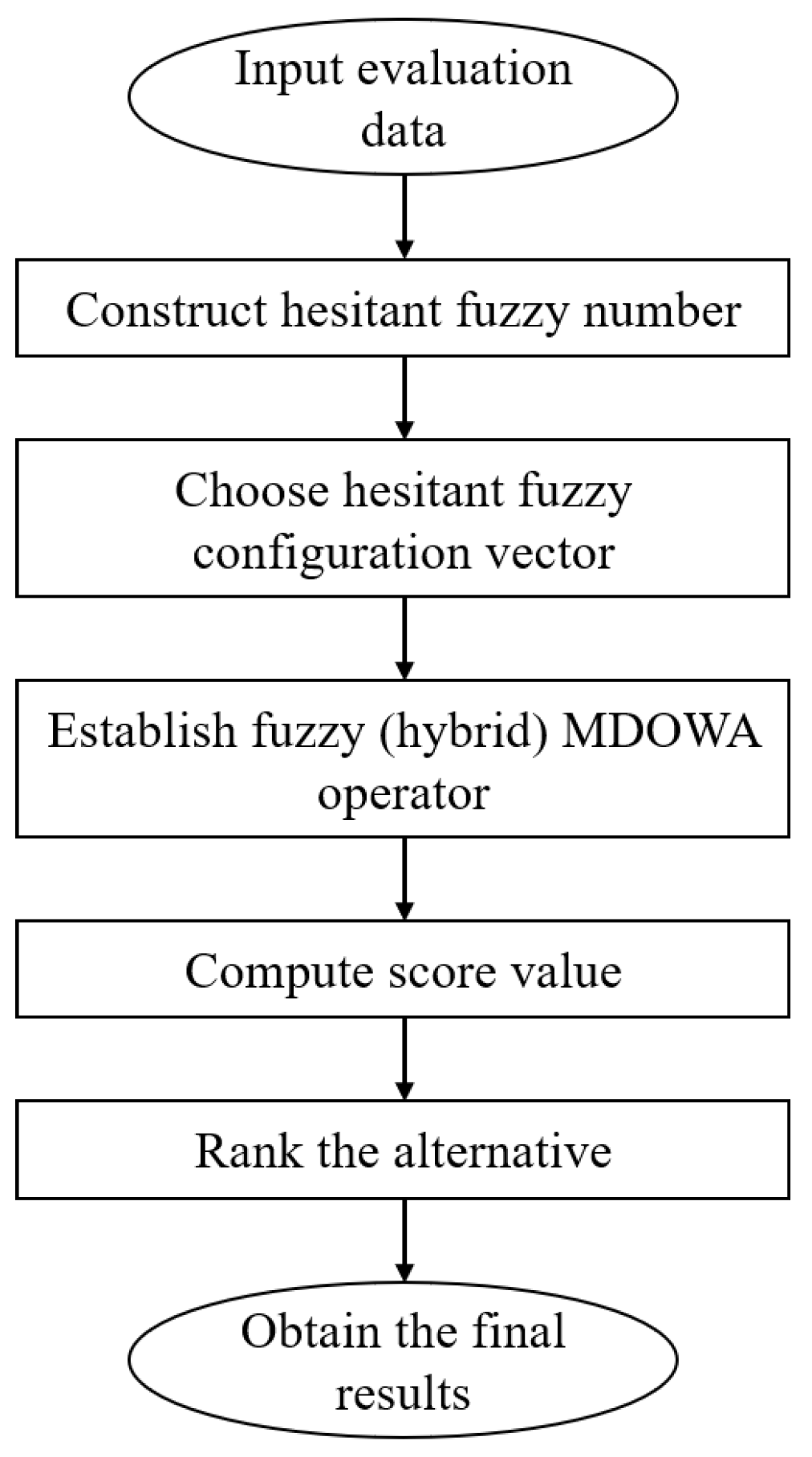
5. Algorithm of Group Decision Making Based on HFMDOWA Operators

Multi-criteria group decision making (MCGDM) can be simply expressed as follows: given m alternatives $B=\{B_1,B_2,\cdots ,B_m\}$, and t experts $E=\{e_1,e_2,\cdots ,e_t\}$ give the evaluations of the alternatives according to the criteria $F=\{f_1,f_2,\cdots ,f_n\}$. Suppose that ${\xi }_{ij}^k\in [0,1](i=1,2,\cdots ,m;j=1,2,\cdots ,n;k=1,2,\cdots ,t)$ is the evaluation of $B_i$ given by $e_k$ considering the criterion $f_j$. The best alternative will be selected by taking into account the evaluations. In what follows, we propose a novel MCGDM method by applying the proposed HFMDOWA operators. To understand steps of this algorithms easily, the flowchart is display in the Figure 1. The algorithm of the presented MCGDM method can be depicted as follows:

Step 1: Considering criterion $f_j$, the evaluations of $B_i$ proposed by all experts construct an HFN ${\tau }_{ij}=\{{\xi }_{ij}^1,{\xi }_{ij}^2,\dots ,{\xi }_{ij}^{p_{ij}}\}(i=1,2,\cdots ,m;j=1,2,\cdots ,n;1\le p_{ij}\le t)$. If two experts give the same evaluation, then the evaluation value can only appear once according to the anonymity of evaluation.

Step 2: Select an appropriate hesitant fuzzy configuration vector, and establish the hesitant fuzzy MDOWA operator or hesitant fuzzy hybrid MDOWA operator.

Step 3: Compute the comprehensive assessment value $M\left(B_i\right)$ of $B_i(i=1,2,\cdots ,m)$ by applying the hesitant fuzzy MDOWA operator or hesitant fuzzy hybrid MDOWA operator.

Step 4: Compute the score value $m\left(M\left(B_i\right)\right)$ of $M\left(B_i\right)(i=1,2,\cdots ,m)$.

Step 5: Rank the alternatives $B_1,B_2,\cdots ,B_m$ by applying $m\left(M\left(B_i\right)\right)(i=1,2,\cdots ,m)$ or select the optimal alternative.

6. Numerical Example

6.1. Description of the Decision Problem

Overall scheme decision-making of warship is a crucial link in the process of warship overall design. It is essential to discuss the schemes in the process of warship overall design. Moreover, since the complexity of warship relates to various knowledge and many qualitative as well as uncertain factors, overall scheme selection needs a group of experts who possess all kinds of knowledge and experience to make group decisions [41]. In what follows, we take part in the warship overall performance index from three aspects, namely, combat capability, logistics support capability, and combat applicability. We consider eleven criteria: ${\wp }_1$: C³I system capability, ${\wp }_2$: antiaircraft combat capability, ${\wp }_3$: antiship combat capability, ${\wp }_4$: antisubmarine combat capability, ${\wp }_5$: habitability, ${\wp }_6$: supply capability, ${\wp }_7$: defense ability against attack from the sea, land, and air, ${\wp }_8$: compatibility, ${\wp }_9$: maneuverability, ${\wp }_{10}$: stealthiness, ${\wp }_{11}$: vitality. The criteria weight vector is $w=(0.1,0.15,0.1,0.1,0.1,0.1,0.05,0.1,0.05,0.1,0.05)$. Suppose five warship overall alternatives ${\Omega }_1,{\Omega }_2,{\Omega }_3,{\Omega }_4,{\Omega }_5$ will be evaluated, and four experts $e_1,e_2,e_3,e_4$ give their evaluations. The evaluation values are shown in

Table 1. The evaluation values provided by expert $e_1$.

	${\mathit{\wp }}_1$	${\mathit{\wp }}_2$	${\mathit{\wp }}_3$	${\mathit{\wp }}_4$	${\mathit{\wp }}_5$	${\mathit{\wp }}_6$	${\mathit{\wp }}_7$	${\mathit{\wp }}_8$	${\mathit{\wp }}_9$	${\mathit{\wp }}_{10}$	${\mathit{\wp }}_{11}$
${\Omega }_1$	0.8	0.6	0.9	0.7	0.6	0.8	0.7	0.9	0.8	0.7	0.6
${\Omega }_2$	0.7	0.9	0.6	0.8	0.7	0.5	0.6	0.9	0.4	0.7	0.6
${\Omega }_3$	0.9	0.6	0.5	0.8	0.7	0.4	0.6	0.5	0.7	0.8	0.9
${\Omega }_4$	0.8	0.5	0.6	0.9	0.7	0.9	0.8	0.4	0.6	0.7	0.5
${\Omega }_5$	0.6	0.8	0.5	0.9	0.9	0.8	0.6	0.5	0.7	0.5	0.8

,

Table 2. The evaluation values provided by expert $e_2$.

	${\mathit{\wp }}_1$	${\mathit{\wp }}_2$	${\mathit{\wp }}_3$	${\mathit{\wp }}_4$	${\mathit{\wp }}_5$	${\mathit{\wp }}_6$	${\mathit{\wp }}_7$	${\mathit{\wp }}_8$	${\mathit{\wp }}_9$	${\mathit{\wp }}_{10}$	${\mathit{\wp }}_{11}$
${\Omega }_1$	0.8	0.5	0.7	0.8	0.9	0.4	0.8	0.6	0.7	0.9	0.5
${\Omega }_2$	0.9	0.8	0.9	0.5	0.4	0.6	0.7	0.5	0.9	0.8	0.7
${\Omega }_3$	0.8	0.6	0.5	0.7	0.9	0.6	0.8	0.7	0.8	0.6	0.7
${\Omega }_4$	0.9	0.6	0.5	0.7	0.8	0.6	0.5	0.5	0.8	0.6	0.8
${\Omega }_5$	0.7	0.8	0.6	0.5	0.9	0.7	0.6	0.8	0.7	0.8	0.6

,

Table 3. The evaluation values provided by expert $e_3$.

	${\mathit{\wp }}_1$	${\mathit{\wp }}_2$	${\mathit{\wp }}_3$	${\mathit{\wp }}_4$	${\mathit{\wp }}_5$	${\mathit{\wp }}_6$	${\mathit{\wp }}_7$	${\mathit{\wp }}_8$	${\mathit{\wp }}_9$	${\mathit{\wp }}_{10}$	${\mathit{\wp }}_{11}$
${\Omega }_1$	0.8	0.6	0.9	0.7	0.8	0.6	0.5	0.9	0.6	0.8	0.7
${\Omega }_2$	0.8	0.7	0.6	0.6	0.8	0.9	0.7	0.6	0.8	0.6	0.8
${\Omega }_3$	0.9	0.5	0.6	0.8	0.7	0.6	0.8	0.9	0.5	0.7	0.6
${\Omega }_4$	0.8	0.6	0.9	0.7	0.7	0.8	0.6	0.5	0.8	0.6	0.7
${\Omega }_5$	0.8	0.6	0.9	0.7	0.8	0.6	0.8	0.9	0.6	0.7	0.6

and

Table 4. The evaluation values provided by expert $e_4$.

	${\mathit{\wp }}_1$	${\mathit{\wp }}_2$	${\mathit{\wp }}_3$	${\mathit{\wp }}_4$	${\mathit{\wp }}_5$	${\mathit{\wp }}_6$	${\mathit{\wp }}_7$	${\mathit{\wp }}_8$	${\mathit{\wp }}_9$	${\mathit{\wp }}_{10}$	${\mathit{\wp }}_{11}$
${\Omega }_1$	0.9	0.8	0.6	0.7	0.9	0.6	0.5	0.8	0.7	0.9	0.7
${\Omega }_2$	0.8	0.5	0.7	0.6	0.9	0.8	0.5	0.7	0.9	0.5	0.8
${\Omega }_3$	0.8	0.6	0.7	0.5	0.9	0.5	0.7	0.6	0.9	0.8	0.7
${\Omega }_4$	0.9	0.5	0.7	0.6	0.8	0.7	0.9	0.5	0.7	0.8	0.6
${\Omega }_5$	0.9	0.6	0.8	0.7	0.5	0.6	0.8	0.9	0.7	0.6	0.8

.

6.2. Evaluation Process

In the following, we deal with above information by applying the proposed algorithm of group decision making.

Step 1: Considering criterion ${\wp }_j(j=1,2,\cdots ,11)$, we merge the evaluation values of ${\Omega }_i(i=1,2,3,4,5)$ provided by experts into a hesitant fuzzy number ${\tau }_{ji}(i=1,2,3,4,5;j=1,2,\cdots ,11)$, which are listed in

Table 5. The HFN values ${\tau }_{ji}$ of the alternatives.

	${\mathbf{\Omega }}_1$	${\mathbf{\Omega }}_2$	${\mathbf{\Omega }}_3$	${\mathbf{\Omega }}_4$	${\mathbf{\Omega }}_5$
${\wp }_1$	$\{0.8,0.9\}$	$\{0.7,0.8,0.9\}$	$\{0.8,0.9\}$	$\{0.8,0.9\}$	$\{0.6,0.7,0.8,0.9\}$
${\wp }_2$	$\{0.5,0.6,0.8\}$	$\{0.5,0.7,0.8,0.9\}$	$\{0.5,0.6\}$	$\{0.5,0.6\}$	$\{0.6,0.8\}$
${\wp }_3$	$\{0.6,0.7,0.9\}$	$\{0.6,0.7,0.9\}$	$\{0.5,0.6,0.7\}$	$\{0.5,0.6,0.7,0.9\}$	$\{0.5,0.6,0.8,0.9\}$
${\wp }_4$	$\{0.7,0.8\}$	$\{0.5,0.6,0.8\}$	$\{0.5,0.7,0.8\}$	$\{0.6,0.7,0.9\}$	$\{0.5,0.7,0.9\}$
${\wp }_5$	$\{0.6,0.8,0.9\}$	$\{0.4,0.7,0.8,0.9\}$	$\{0.7,0.9\}$	$\{0.7,0.8\}$	$\{0.5,0.8,0.9\}$
${\wp }_6$	$\{0.4,0.6,0.8\}$	$\{0.5,0.6,0.8,0.9\}$	$\{0.4,0.5,0.6\}$	$\{0.6,0.7,0.8,0.9\}$	$\{0.6,0.7,0.8\}$
${\wp }_7$	$\{0.5,0.7,0.8\}$	$\{0.5,0.6,0.7\}$	$\{0.6,0.7,0.8\}$	$\{0.5,0.6,0.8,0.9\}$	$\{0.6,0.8\}$
${\wp }_8$	$\{0.6,0.8,0.9\}$	$\{0.5,0.6,0.7,0.9\}$	$\{0.5,0.6,0.7,0.9\}$	$\{0.4,0.5\}$	$\{0.5,0.8,0.9\}$
${\wp }_9$	$\{0.6,0.7,0.8\}$	$\{0.4,0.8,0.9\}$	$\{0.5,0.7,0.8,0.9\}$	$\{0.6,0.7,0.8\}$	$\{0.6,0.7\}$
${\wp }_{10}$	$\{0.7,0.8,0.9\}$	$\{0.5,0.6,0.7,0.8\}$	$\{0.6,0.7,0.8\}$	$\{0.6,0.7,0.8\}$	$\{0.5,0.6,0.7,0.8\}$
${\wp }_{11}$	$\{0.5,0.6,0.7\}$	$\{0.6,0.7,0.8\}$	$\{0.6,0.7,0.9\}$	$\{0.5,0.6,0.7,0.8\}$	$\{0.6,0.8\}$

.

In what follows, we calculate the weighted HFNs and their score values which are given in

Table 6. The weighted HFN values ${\tilde{\tau }}_{ji}$ of the alternatives.

	${\mathbf{\Omega }}_1$	${\mathbf{\Omega }}_2$	${\mathbf{\Omega }}_3$	${\mathbf{\Omega }}_4$	${\mathbf{\Omega }}_5$
${\wp }_1$	$\{0.1487,0.2057\}$	$\{0.1134,0.1487,0.2057\}$	$\{0.1487,0.2057\}$	$\{0.1487,0.2057\}$	$\{0.0876,0.1134,0.1487,0.2057\}$
${\wp }_2$	$\{0.0987,0.1284,0.2145\}$	$\{0.0987,0.1652,0.2145,0.2921\}$	$\{0.0987,0.1284\}$	$\{0.0987,0.1284\}$	$\{0.1284,0.2145\}$
${\wp }_3$	$\{0.0876,0.1134,0.2057\}$	$\{0.0876,0.1134,0.2057\}$	$\{0.0670,0.0876,0.1134\}$	$\{0.0670,0.0876,0.1134,0.2057\}$	$\{0.0670,0.0876,0.1487,0.2057\}$
${\wp }_4$	$\{0.1134,0.1487\}$	$\{0.0670,0.0876,0.1487\}$	$\{0.0670,0.1134,0.1487\}$	$\{0.0876,0.1134,0.2057\}$	$\{0.0670,0.1134,0.2057\}$
${\wp }_5$	$\{0.0876,0.1487,0.2057\}$	$\{0.0498,0.1134,0.1487,0.2057\}$	$\{0.1134,0.2057\}$	$\{0.1134,0.1487\}$	$\{0.0670,0.1487,0.2057\}$
${\wp }_6$	$\{0.0498,0.0876,0.1487\}$	$\{0.0670,0.0876,0.1487,0.2057\}$	$\{0.0498,0.0670,0.0876\}$	$\{0.0876,0.1134,0.1487,0.2057\}$	$\{0.0876,0.1134,0.1487\}$
${\wp }_7$	$\{0.0341,0.0584,0.0773\}$	$\{0.0341,0.0448,0.0584\}$	$\{0.0448,0.0584,0.0773\}$	$\{0.0341,0.0448,0.0773,0.1087\}$	$\{0.0448,0.0773\}$
${\wp }_8$	$\{0.0876,0.1487,0.2057\}$	$\{0.0670,0.0876,0.1134,0.2057\}$	$\{0.0670,0.0876,0.1134,0.2057\}$	$\{0.0498,0.0670\}$	$\{0.0670,0.1487,0.2057\}$
${\wp }_9$	$\{0.0448,0.0584,0.0773\}$	$\{0.0252,0.0773,0.1087\}$	$\{0.0341,0.0584,0.0773,0.1087\}$	$\{0.0448,0.0584,0.0773\}$	$\{0.0448,0.0584\}$
${\wp }_{10}$	$\{0.1134,0.1487,0.2057\}$	$\{0.0670,0.0876,0.1134,0.1487\}$	$\{0.0876,0.1134,0.1487\}$	$\{0.0876,0.1134,0.1487\}$	$\{0.0670,0.0876,0.1134,0.1487\}$
${\wp }_{11}$	$\{0.0341,0.0448,0.0584\}$	$\{0.0448,0.0584,0.0773\}$	$\{0.0448,0.0584,0.1087\}$	$\{0.0341,0.0448,0.0584,0.0773\}$	$\{0.0448,0.0773\}$

and

Table 7. The score values of the weighted HFNs.

	${\mathit{\wp }}_1$	${\mathit{\wp }}_2$	${\mathit{\wp }}_3$	${\mathit{\wp }}_4$	${\mathit{\wp }}_5$	${\mathit{\wp }}_6$	${\mathit{\wp }}_7$	${\mathit{\wp }}_8$	${\mathit{\wp }}_9$	${\mathit{\wp }}_{10}$	${\mathit{\wp }}_{11}$
${\Omega }_1$	0.1772	0.1472	0.1356	0.1310	0.1473	0.0954	0.0566	0.1473	0.0602	0.1559	0.0458
${\Omega }_2$	0.1559	0.1926	0.1356	0.1011	0.1294	0.1273	0.0458	0.1184	0.0704	0.1042	0.0602
${\Omega }_3$	0.1772	0.1135	0.0893	0.1097	0.1595	0.0681	0.0602	0.1184	0.0696	0.1166	0.0706
${\Omega }_4$	0.1772	0.1135	0.1184	0.1356	0.1310	0.1389	0.0662	0.0584	0.0602	0.1166	0.0537
${\Omega }_5$	0.1389	0.1714	0.1273	0.1287	0.1405	0.1166	0.0610	0.1405	0.0516	0.1042	0.0610

, respectively.

Step 2: Select the appropriate hesitant fuzzy configuration vector. Considering the specificity of warship’s task, each criterion should be satisfied as much as possible. Hence, we select the hesitant fuzzy balanced configuration vector to obtain the variable weights. To this end, we utilize the balanced primary function ${\displaystyle M\left(c\right)={\sum }_{k=1}^5(9+\frac{e^{\delta c_k}}{\delta })(\delta <0)}$ to obtain the balanced configuration vector. Since each criterion should be satisfied as much as possible, we apply the balanced HFHMDOWA operators to synthesize the HFNs.

Step 3: Calculate the synthesis values of ${\Omega }_k(k=1,2,3,4,5)$ by using the hesitant fuzzy hybrid MDOWA operator. To demonstrate the virtues of the presented method, we select different values of $\delta$ to construct different balanced HFHMDOWA operators. By applying Equations (12) and (15), the assessment values are obtained. For each alternative ${\Omega }_k(k=1,2,3,4,5)$, we do not give the overall synthesized results $\mathrm{HFHMDOWA}\left({\Omega }_k\right)$ because of vast amounts of data and limited space. Then we compute the score values of $\mathrm{HFHMDOWA}\left({\Omega }_k\right)(k=1,2,3,4,5)$. For convenience, the score value $m\left(\mathrm{HFHMDOWA}\left({\Omega }_k\right)\right)$ is simply represented as $m\left({\Omega }_k\right)$. The results provided by HFHMDOWA(I) operators and HFHMDOWA(II) operators are shown in

Table 8. Results provided by different HFHMDOWA(I) operators.

	$\mathit{m}\left({\mathbf{\Omega }}_1\right)$	$\mathit{m}\left({\mathbf{\Omega }}_2\right)$	$\mathit{m}\left({\mathbf{\Omega }}_3\right)$	$\mathit{m}\left({\mathbf{\Omega }}_4\right)$	$\mathit{m}\left({\mathbf{\Omega }}_5\right)$	Ranking Results
$\delta =-5.5$	0.10904	0.10554	0.09906	0.09939	0.10648	${\Omega }_1\succ {\Omega }_5\succ {\Omega }_2\succ {\Omega }_4\succ {\Omega }_3$
$\delta =-4.5$	0.11100	0.10721	0.10025	0.10088	0.10806	${\Omega }_1\succ {\Omega }_5\succ {\Omega }_2\succ {\Omega }_4\succ {\Omega }_3$
$\delta =-3.5$	0.11299	0.10888	0.10149	0.10239	0.10949	${\Omega }_1\succ {\Omega }_5\succ {\Omega }_2\succ {\Omega }_4\succ {\Omega }_3$
$\delta =-2.5$	0.11499	0.11057	0.10275	0.10390	0.11098	${\Omega }_1\succ {\Omega }_5\succ {\Omega }_2\succ {\Omega }_4\succ {\Omega }_3$
$\delta =-1.5$	0.11709	0.11227	0.10405	0.10542	0.11243	${\Omega }_1\succ {\Omega }_5\succ {\Omega }_2\succ {\Omega }_4\succ {\Omega }_3$
$\delta =-0.5$	0.11896	0.11398	0.10537	0.10694	0.11396	${\Omega }_1\succ {\Omega }_2\succ {\Omega }_5\succ {\Omega }_4\succ {\Omega }_3$
$\delta =-0.2$	0.11956	0.11449	0.10578	0.10740	0.11424	${\Omega }_1\succ {\Omega }_2\succ {\Omega }_5\succ {\Omega }_4\succ {\Omega }_3$
$\delta =-0.1$	0.11968	0.11467	0.10591	0.10755	0.11442	${\Omega }_1\succ {\Omega }_2\succ {\Omega }_5\succ {\Omega }_4\succ {\Omega }_3$

and

Table 9. Results provided by different HFHMDOWA(II) operators.

	$\mathit{m}\left({\mathbf{\Omega }}_1\right)$	$\mathit{m}\left({\mathbf{\Omega }}_2\right)$	$\mathit{m}\left({\mathbf{\Omega }}_3\right)$	$\mathit{m}\left({\mathbf{\Omega }}_4\right)$	$\mathit{m}\left({\mathbf{\Omega }}_5\right)$	Ranking Results
$\delta =-5.5$	0.10350	0.09756	0.09508	0.09531	0.09945	${\Omega }_1\succ {\Omega }_5\succ {\Omega }_2\succ {\Omega }_4\succ {\Omega }_3$
$\delta =-4.5$	0.10634	0.10036	0.09690	0.09740	0.10198	${\Omega }_1\succ {\Omega }_5\succ {\Omega }_2\succ {\Omega }_4\succ {\Omega }_3$
$\delta =-3.5$	0.10926	0.10331	0.09880	0.09957	0.10462	${\Omega }_1\succ {\Omega }_5\succ {\Omega }_2\succ {\Omega }_4\succ {\Omega }_3$
$\delta =-2.5$	0.11225	0.10641	0.10078	0.10181	0.10736	${\Omega }_1\succ {\Omega }_5\succ {\Omega }_2\succ {\Omega }_4\succ {\Omega }_3$
$\delta =-1.5$	0.11528	0.10967	0.10283	0.10412	0.11018	${\Omega }_1\succ {\Omega }_5\succ {\Omega }_2\succ {\Omega }_4\succ {\Omega }_3$
$\delta =-0.5$	0.11836	0.11308	0.10496	0.10650	0.11309	${\Omega }_1\succ {\Omega }_5\succ {\Omega }_2\succ {\Omega }_4\succ {\Omega }_3$
$\delta =-0.2$	0.11929	0.11413	0.10561	0.10722	0.11398	${\Omega }_1\succ {\Omega }_2\succ {\Omega }_5\succ {\Omega }_4\succ {\Omega }_3$
$\delta =-0.1$	0.11960	0.11448	0.10583	0.10746	0.11427	${\Omega }_1\succ {\Omega }_2\succ {\Omega }_5\succ {\Omega }_4\succ {\Omega }_3$

, respectively.

By analyzing the above results, it can be easily seen that the parameter values in the primary function affect the final ranking results. According to the results provided by Zeng et al. in literature [25], it is known that the greater the value of $\delta$ in primary function, the nearer the corresponding MDOWA operator is to the maximum operator, and as its value is smaller, the corresponding MDOWA operator is nearer to the minimization operator. Therefore, if organizers can pick out the appropriate value of $\delta$ on the basis of their attitude characters, the presented HFHMDOWA operators will provide much precise decision results. Hence, the proposed HFHMDOWA operators are much more effective and adaptive to deal with hesitant fuzzy information since the decision makers have much more opportunities to reflect their true thoughts.

Remark 2.

It is not difficult to understand that the selection of the appropriate parameters used for HFMDOWA and HFHMDOWA operators is very crucial in practical application. Aforementioned ranking results show that the parameters in primary function have great influence on the final results, which is mainly reflected in getting different variable weights. Hence, we can obtain the parameters in primary function by using the methods of determining the weight in the OWA operator [15,42], which is the content of our future research.

6.3. Comparison with HFWA Operator Developed by Xia and Xu [10]

To demonstrate the rationality of the presented HFHMDOWA operators, in the following, we utilize the HFWA operator provided by Xia and Xu [10] to synthesize the aforementioned HFNs.

A: Results calculated by HFWA operator

The hesitant fuzzy weighted averaging (HFWA) operator proposed by Xia and Xu [10] is a common operator for integrating hesitant fuzzy information. In the following, we calculate the synthesized values of the above HFNs by utilizing Equation (1). Similarly, we also do not list the synthesized values and only give the score values of the corresponding HFNs. For convenience, we denote the score value of the aggregated value of alternative ${\Omega }_k$ as $m\left(\mathrm{HFWA}\left({\Omega }_k\right)\right)(k=1,2,3,4,5)$. After calculations, we have

$$m\left(\mathrm{HFWA}\left({\Omega }_1\right)\right)=0.7409,m\left(\mathrm{HFWA}\left({\Omega }_2\right)\right)=0.7049,m\left(\mathrm{HFWA}\left({\Omega }_3\right)\right)=0.7006,$$

$$m\left(\mathrm{HFWA}\left({\Omega }_4\right)\right)=0.7091,m\left(\mathrm{HFWA}\left({\Omega }_5\right)\right)=0.7119$$

Then we have ${\Omega }_1\succ {\Omega }_5\succ {\Omega }_4\succ {\Omega }_2\succ {\Omega }_3$, which is different from the results provided by the presented HFHMDOWA operators.

B: Discussion

In the previous example, the ranking result obtained by the HFWA operator is different from those obtained by the proposed HFHMDOWA operators. When $\delta \le -1.5$, the ranking results of the alternatives provided by these three methods are slightly different, with the main difference lying in ${\Omega }_2$ and ${\Omega }_4$. The former result is ${\Omega }_2\succ {\Omega }_4$, while the latter is ${\Omega }_4\succ {\Omega }_2$. When $\delta =-0.5$, the ranking results of the alternatives provided by the HFWA operator and the HFHMDOWA(I) operator are quite different. When $\delta \ge -0.2$, the ranking results obtained by HFHMDOWA(I) operator and HFHMDOWA(II) operator are the same, but the difference between the results obtained by HFHMDOWA operators and HFWA operators is even greater. In this case, the ranking results of ${\Omega }_2,{\Omega }_4$, and ${\Omega }_5$ have all changed, with the former being ${\Omega }_2\succ {\Omega }_5\succ {\Omega }_4$, and the latter being ${\Omega }_5\succ {\Omega }_4\succ {\Omega }_2$. These differences just show the flexibility and rationality of the presented operators.

7. Conclusions

DOWA operators take into account the overall influences of the aggregated elements. Therefore, they can fully express the impact of the internal relations of the synthesized values. HFSs that permit the membership, including different values, are able to describe human’s hesitation effectively. HFS theory has become a very powerful tool to handle complex information. To aggregate hesitant fuzzy information more effectively, we develop several HFMDOWA operators to aggregate HFNs in this paper, such as BAL-HFMDOWA operators, REW-HFMDOWA operators, BAL-HFHMDOWA operators, and REW-HFHMDOWA operators. The variable weights of the presented operators are obtained and revised automatically. Hence, the proposed aggregation operators can express the decision maker’s preferences fully.

Owing to the proposed method providing a novel operator in group decision-making tasks, this operator still exists following drawbacks. The parameters of the proposed method need to be determined suitably. On the other hand, this operator needs to generalize more real application fields. In the future, we will further study the method of picking out more suitable parameter values in primary functions when hesitant fuzzy information is aggregated in order to utilize the proposed HFMDOWA operators more efficiently. And we will give more application fields examples, especially for financial decision-making and supply chain management.

References

1. Herrera, F.; Herrera-Viedma, E. Aggregation operators for linguistic weighted information. IEEE Trans. Syst. Man Cybern. Part A 1997, 22, 646–656. [Google Scholar] [CrossRef]
2. Xu, Z.S.; Da, Q.L. An overview of operators for aggregating information. Int. J. Intell. Syst. 2003, 18, 953–969. [Google Scholar] [CrossRef]
3. Chen, S.J.; Chen, S.M. A new method for handling multicriteria fuzzy decision making problems using FN-IOWA operators. Cybern. Syst. 2003, 34, 109–137. [Google Scholar] [CrossRef]
4. Herrera, F.; Herrera-Viedma, E.; Chiclana, F. A study of the origin and uses of the ordered weighted geometric operator in multicriteria decision making. Int. J. Intell. Syst. 2003, 18, 689–707. [Google Scholar] [CrossRef]
5. Marques Pereira, R.A.; Ribeiro, R.A. Aggregation with generalized mixture operators using weighting functions. Fuzzy Sets Syst. 2003, 137, 43–58. [Google Scholar] [CrossRef]
6. Yager, R.R. On ordered weighted averaging aggregation operators in multiciteria decision making. IEEE Trans. Syst. Man Cybern. 1988, 18, 183–190. [Google Scholar] [CrossRef]
7. Yager, R.R. Families of OWA operators. Fuzzy Sets Syst. 1993, 59, 125–148. [Google Scholar] [CrossRef]
8. Yager, R.R. Generalized OWA Aggregation operators. Fuzzy Optim. Decis. Mak. 2004, 3, 93–107. [Google Scholar] [CrossRef]
9. Torra, V. OWA operators in data modeling and reidentification. IEEE Trans. Fuzzy Syst. 2004, 12, 652–660. [Google Scholar] [CrossRef]
10. Xia, M.M.; Xu, Z.S. Hesitant fuzzy information aggregation in decision making. Int. J. Approx. Reason. 2011, 52, 395–407. [Google Scholar] [CrossRef]
11. Liu, X.W.; Lou, H.W. Parameterized additive neat OWA operators with different orness levels. Int. J. Intell. Syst. 2006, 21, 1045–1072. [Google Scholar] [CrossRef]
12. Fernández Salido, J.M.; Murakami, S. Extending Yager’s orness concept for the OWA aggregators to other mean operators. Fuzzy Sets Syst. 2003, 139, 515–542. [Google Scholar] [CrossRef]
13. Liu, X.W. The orness measures for two compound quasi-arithmetic mean aggregation operators. Int. J. Approx. 2010, 51, 305–334. [Google Scholar] [CrossRef]
14. Paternain, D.; Ochoa, G.; Lizasoain, I.; Bustince, H.; Mesiar, R. Quantitative orness for lattice OWA operators. Inf. Fusion 2016, 30, 27–35. [Google Scholar] [CrossRef]
15. Filev, D.P.; Yager, R.R. On the issue of obtaining OWA operator weights. Fuzzy Sets Syst. 1998, 94, 157–169. [Google Scholar] [CrossRef]
16. Ahn, B.S. On the properties of OWA operator weights functions with constant level of orness. IEEE Trans. Fuzzy Syst. 2006, 14, 511–515. [Google Scholar] [CrossRef]
17. Sang, X.Z.; Liu, X.W. An analytic approach to obtain the least square deviation OWA operator weights. Fuzzy Sets Syst. 2014, 240, 103–116. [Google Scholar] [CrossRef]
18. Fullér, R.; Majlender, P. An analytic approach for obtaining maximal entropy OWA operator weights. Fuzzy Sets Syst. 2001, 124, 53–57. [Google Scholar] [CrossRef]
19. Torra, V. The weighted OWA operator. Int. J. Intell. Syst. 1997, 12, 153–166. [Google Scholar] [CrossRef]
20. Yager, R.R. OWA aggregation over a continuous interval argument with applications to decision making. IEEE Trans. Syst. Man Cybern. Part B 2004, 34, 1952–1963. [Google Scholar] [CrossRef]
21. Yager, R.R. Centered OWA operators, Soft Computing: A Fusion of Foundations. Methodol. Appl. 2007, 11, 631–639. [Google Scholar] [CrossRef]
22. Llamazares, B. Constructing Choquet integral-based operators that generalize weighted means and OWA operators. Inf. Fusion 2015, 23, 131–138. [Google Scholar] [CrossRef]
23. Llamazares, B. SUOWA operators: Constructing semi-uninorms and analyzing specific cases. Fuzzy Sets Syst. 2016, 287, 119–136. [Google Scholar] [CrossRef]
24. Xu, Z.S. Dependent uncertain ordered weighted aggregation operators. Inf. Fusion 2008, 9, 310–316. [Google Scholar] [CrossRef]
25. Zeng, W.Y.; Li, D.Q.; Gu, Y.D. Monotonic argument dependent OWA operators. Int. J. Intell. Syst. 2018, 33, 1639–1659. [Google Scholar] [CrossRef]
26. Zadeh, L.A. Fuzzy sets. Inf. Control 1965, 8, 338–356. [Google Scholar] [CrossRef]
27. Torra, V. Hesitant fuzzy sets. Int. J. Intell. Syst. 2010, 25, 529–539. [Google Scholar] [CrossRef]
28. Wei, G.W. Hesitant fuzzy prioritized operators and their application to multiple attribute decision making. Knowl.-Based Syst. 2012, 31, 176–182. [Google Scholar] [CrossRef]
29. Chen, N.; Xu, Z.S.; Xia, M.M. Correlation coefficients of hesitant fuzzy sets and their applications to clustering analysis. Appl. Math. Model. 2013, 37, 2197–2211. [Google Scholar] [CrossRef]
30. Zhang, Z.M. Hesitant fuzzy power aggregation operators and their application to multiple attribute group decision making. Inf. Sci. 2013, 234, 150–181. [Google Scholar] [CrossRef]
31. Zhu, B.; Xu, Z.S.; Xia, M.M. Hesitant fuzzy geometric Bonferroni means. Inf. Sci. 2012, 182, 72–85. [Google Scholar] [CrossRef]
32. Chen, N.; Xu, Z.S.; Xia, M.M. Interval-valued hesitant preference relations and their applications to group decision making. Knowl.-Based Syst. 2013, 37, 528–540. [Google Scholar] [CrossRef]
33. Rodríguez, R.M.; Martínez, L.; Herrera, F. Hesitant fuzzy linguistic term sets for decision making. IEEE Trans. Fuzzy Syst. 2012, 20, 109–119. [Google Scholar] [CrossRef]
34. Li, D.Q.; Zeng, W.Y.; Li, J.H. New distance and similarity measures on hesitant fuzzy sets and their applications in multiple criteria decision making. Eng. Appl. Artif. Intell. 2015, 40, 11–16. [Google Scholar] [CrossRef]
35. Li, D.Q.; Zeng, W.Y.; Zhao, Y.B. Note on distance measure of hesitant fuzzy sets. Inf. Sci. 2015, 321, 103–115. [Google Scholar] [CrossRef]
36. Zeng, W.Y.; Li, D.Q.; Yin, Q. Distance and similarity measures of hesitant fuzzy sets and their application in pattern recognition. Pattern Recognit. Lett. 2016, 84, 267–271. [Google Scholar] [CrossRef]
37. Qahtan, S.; Alsattar, H.A.; Zaidan, A.A.; Deveci, M.; Pamucar, D.; Ding, W.P. A novel fuel supply system modelling approach for electric vehicles under Pythagorean probabilistic hesitant fuzzy sets. Inf. Sci. 2023, 622, 1014–1032. [Google Scholar] [CrossRef]
38. Fang, B. Some uncertainty measures for probabilistic hesitant fuzzy information. Inf. Sci. 2023, 625, 255–276. [Google Scholar] [CrossRef]
39. Saha, A.; Simic, V.; Senapati, T.; Miletic, S.D.; Ala, A. A dual hesitant fuzzy sets-based methodology for advantage prioritization of zero-emission last-mile delivery solutions for sustainable city logistics. IEEE Trans. Fuzzy Syst. 2023, 31, 407–420. [Google Scholar] [CrossRef]
40. Liao, H.C.; Xu, Z.S.; Xia, M.M. Multiplicative consistency of hesitant fuzzy preference relation and its application in group decision making. Int. J. Inf. Technol. Decis. Mak. 2014, 13, 47–76. [Google Scholar] [CrossRef]
41. Guo, H.P.; Huang, S.; Wang, C. Group decision making method of warship overall scheme based on improved Delphi. J. Shanghai Jiao Tong Univ. 2014, 48, 515–519. (In Chinese) [Google Scholar] [CrossRef]
42. Xu, Z.S. An Overview of Methods for Determining OWA Weights. Int. J. Intell. Syst. 2005, 20, 843–865. [Google Scholar] [CrossRef]
Figure 1. Flowchart of the proposed method.
Symmetry 16 01450 g001