1. Introduction
The outbreak of the novel coronavirus COVID-19 in China at the end of 2019 has attracted extensive attention from many scientists, in particular mathematicians working in mathematical modeling. At the present time, there are thousands of research papers and dozens of books devoted to mathematical modeling of the COVID-19 pandemic. However, there is a relatively small number of papers in which space distributed models are applied to understand the pandemic’s spread (see review [
1] and the papers cited therein). Moreover, the above number is essentially reduced if one looks for studies devoted to the application of space distributed models for COVID-19 pandemic modeling in specific countries. We were able to identify the works [
2,
3,
4,
5,
6,
7,
8,
9,
10,
11,
12,
13,
14,
15] in which some comparison between the results of numerical simulations (using the space distributed models) and the official data were presented.
The main aim of this study is to demonstrate the applicability of the space distributed model based on reaction–diffusion equations as developed in [
16] and further studied in [
17] in the case of the second pandemic wave in Ukraine. It should be noted that there are several studies devoted to the mathematical modeling of the COVID-19 pandemic in Ukraine (see [
18,
19,
20] and the references cited therein). However, the mathematical models used therein are based on ordinary differential equations (ODEs), which coincide with the classical Susceptible-Infected-Recovered (SIR) model [
21] or are its direct generalizations used by other authors (see, e.g., [
22,
23,
24,
25]). To the best of our knowledge, this study is the first in which the mathematical modeling of the COVID-19 pandemic in Ukraine is based on a model involving partial differential equations. Moreover, we show that the model suggested earlier should be generalized before its application to the pandemic spread modeling.
It should be stressed that the official data of the Ministry of Health of Ukraine concerning the number of COVID-19 cases in the first half of 2020 can be essentially incorrect because of very low numbers of COVID-19 tests at that time. Therefore, we decided to apply the model to the second wave, which can be identified on plots presented in the data source [
26]. One may conclude that the second wave took place in Ukraine in the first half of 2021. Notably, the vaccination process against the SARS-CoV-2 virus widely started only in the summer of 2021; therefore, this factor had no impact on the second wave of the COVID-19 process in Ukraine and was not taken into account in the model.
The paper is organized as follows. In
Section 2, a geometrical approximation of the shape of Ukraine is worked out. It is an important step because its geographical borders have very complicated forms. In
Section 3, the mathematical model is formulated, and interpretation of the parameters arising in the model is presented. In
Section 4, we show how the initial conditions can be identified using the known official data for the total number of COVID-19 cases and deaths. In
Section 5, some theoretical analysis and the results of preliminary numerical simulations are presented, which demonstrate that the model studied earlier in [
17] must be generalized. Analytical and approximate formulas for parameters arising in the model are derived as well. In
Section 6, the results of numerical simulations of the generalized model are presented and analyzed. In particular, comparison with the numerical results obtained from the official data shows that the model is adequate and produces very plausible total numbers of COVID-19 cases and deaths during the second wave in Ukraine. In
Section 7, a simplification of the model is analyzed. The results obtained demonstrate that the model is still applicable; however, comparison with the official data leads to less optimistic conclusions. Finally, we discuss the results obtained and present some conclusions in the last section. In particular, we discuss how the results obtained can be improved via further analysis of the parameters arising in the model.
2. The Second Pandemic Wave and a Geometrical Approximation of the Form of Ukraine
According to the official data from [
27] that are almost identical to those presented in [
26], the second wave of the COVID-19 pandemic in Ukraine lasted from the beginning of February 2021 until the middle of July 2021. To model the dynamics of this wave, it is necessary to identify the moments marking the wave start, the peak, and the end. We generate these moments using the relevant numbers of new COVID-19 cases per day from [
26]. Notably, the seven-day moving average (approximation) was used.
As a result, the start of the wave is taken as 7 February 2021. That is the initial point
days, when the following local minimum of new cases per day was recorded—3628 people [
26]. The peak of the wave is identified as 9 April 2021 (
days), when the number of new cases reached a local maximum of 16,006 people. The end of the wave could be fixed as the date 14 July 2021, when the number of new cases reached the next local minimum of 467 people (
days). The time point
days, corresponding to 18 May 2021, was also used because it marks the end of the rapid increase in COVID-19 cases, i.e., this is the beginning of the ’plateau’.
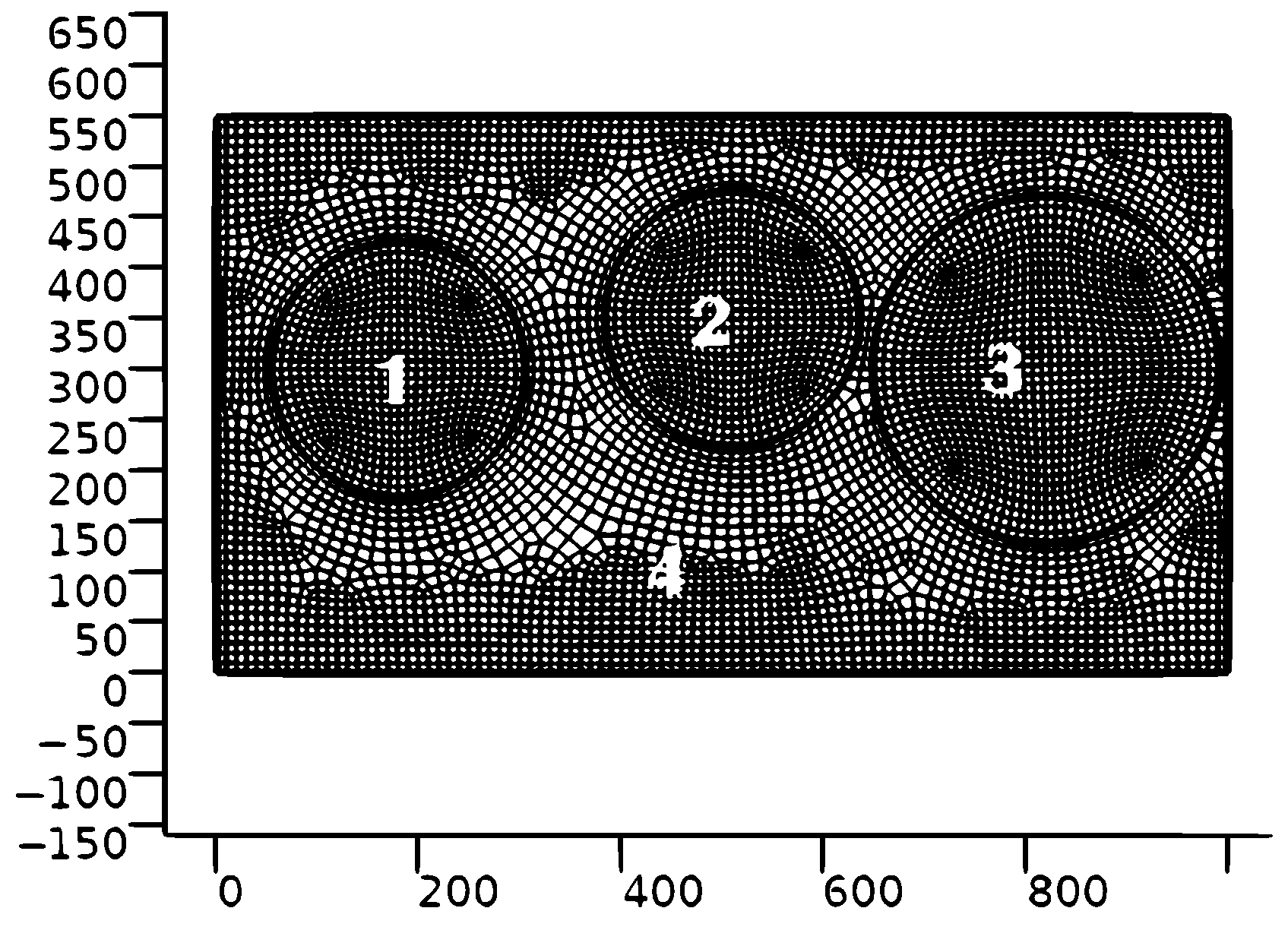
The geometrical shape of Ukraine is very complicated. First of all, the shape of Ukraine (excluding the temporarily occupied territories (TOTs) in 2021) is approximated by the rectangle
with the area
S = 1000 × 550 = 550,000
. The area of Ukraine is divided into four regions:
, consisting of the Ivano-Frankivsk, Lviv, and Ternopil Regions;
, consisting of the Kyiv City, Kyiv, and Cherkasy Regions;
, consisting of the Dnipropetrovsk, Poltava, and Kharkiv Regions; and
, which takes into account the rest of the territory of Ukraine. These four regions are named West, Kyiv, East, and Rest, respectively. The actual areas of the above-mentioned regions are:
,
, and
, respectively. Thus, one concludes that
Geometrical forms of the first three regions were selected as the rings with the centers (see
Figure 1)
Obviously, the geometrical approximation of the shape of Ukraine presented above has low exactness. However, we were motivated by the official data concerning the second wave. In fact, the number of COVID-19 cases were the largest in these three regions. It should be also noted that population sizes in these regions were taken into account as well.
4. Identification of Initial Profiles
We assume that the total number of new COVID-19 cases
and deaths
, from
the beginning of the second wave to time
t, are caused only by the number of active cases in Ukraine at the beginning of this wave. Now, we turn to approximation of the functions
and
using this assumption. The number of active cases up to the time
t is determined by the formula
where
,
, and
are the total number of COVID-19 cases, deaths, and recovered persons from
the beginning of the epidemic up to time
t, respectively. Thus, using the data from [
26], the initial condition for
in the beginning of the second wave can be taken as
Initial conditions for regions 1, 2, 3, and 4 can be also specified in the same way as for the entire country using the data from each region presented in [
27]. The initial number of deaths was determined as the difference between the relevant numbers declared on 7 February 2021 and 6 February 2021 [
27]. All the numbers obtained are summarized in
Table 2.
The average numbers
and
were used as initial data for the region Rest (see the last column of
Table 2) because the pandemic spread during the second wave in Ukraine affected mostly the large cities regions 1, 2, and 3. Thus, homogeneous densities
and
in this region are an obvious choice. The initial conditions for the regions West, Kyiv, and East, in contrast to the region Rest, cannot be taken as constants and are specified in the form of spherically-symmetric surfaces with the centers (see Formulae (
1)). A reasonable choice for creating such surfaces is the cos function in the form
As a result, we arrive at the formulae
where
, and
are specified below.
It should be stressed that data for Ukraine presented in [
26] should be adapted to the second wave. It means that the number of COVID-19 cases during the second wave should be calculated as follows:
where the total number from the beginning of the COVID-19 pandemic,
, is given in [
26]. Thus, taking into account that
and
we obtain
In the same way, the official number of COVID-19 cases during the second wave should be calculated for regions 1, 2, 3, and 4 using the official data presented in [
27].
As indicated above, the initial numbers of deaths in the beginning of the second wave can be determined via the formula
where the numbers
and
correspond to 7 February 2021 and 6 February 2021, respectively, and they are given in [
26]. Finally, the total number of deaths during the second wave up to the time
t is
The analogous numbers for regions 1, 2, 3, and 4 were taken from [
27]. Equations (
9)–(
11) are applicable for each region as well. All the numbers derived are summarized in
Table 3.
Similar to the obtained Equations (
9) and (
11) for determining the number of infected persons and deaths in all of Ukraine, we derive formulas for determining these numbers in each region:
and
Here, we used data related to each region of Ukraine from the report of the working group of the National Academy of Science of Ukraine. The group conducted the mathematical modeling of the SARS-CoV-2 coronavirus epidemic in Ukraine [
27].
As a result, taking into account the average densities
and
(see
Table 2) and the initial total number of COVID-19 infections and deaths in each region (see
Table 3), the constants arising in the initial conditions (
7) and (
8) can be calculated as follows:
5. Numerical Simulations: Preliminaries
First of all, we present the following observation. The nonlinear boundary value problem (BVP)—Equations (
2), (
3), (
5) and (
6)—involves the no-flux conditions (
5). Moreover, the governing Equation (
2) has the constant steady state
, which is stable. As a result, taking into account Equation (
3), one should expect the following asymptotic behavior of solutions to this nonlinear BVP:
where
is a constant.
The above observation was verified by numerical simulations using different forms of the initial profiles by Equation (
6) (see the next section). Obviously, the asymptotic behavior of Equation (
12) can occur in small countries during the COVID-19 pandemic spread; however, that is not plausible in the case of countries such as Ukraine because the large country area leads to essential space inhomogeneity. Thus, the governing Equations (
2) and (
3) should be generalized in order to obtain an adequate model describing the COVID-19 pandemic spread in Ukraine. Here we propose to use step-wise functions for the parameters
and
. This means that these parameters can take different values in different regions, that is
where the relevant parameters with a subscript
i should be defined for each region.
In the general case, the governing Equations (
2) and (
3) can be generalized as follows:
where
, and
are some nonnegative functions.
In order to start numerical simulations, one needs to specify the initial values of parameters arising in the model. First of all, we decided to fix
because this value was already used in [
16] for modeling the COVID-19 pandemic in China. Moreover, the first line in Equation (
2) with
is the famous Fisher equation [
28]
hence, our results may have broader applicability.
Taking into account interpretation of the parameters, we believe that the parameter
a does not vary as much as
b and can be specified (or at least estimated with a sufficient exactness) as follows. Assuming that the density
u of the COVID-19 cases in the initial period of the wave is approximately homogeneous in space, one may consider, instead of Equation (
15), the ODE
which is, of course, the logistic equation with a well-known exact solution. This solution for a short time can be approximated as
. Therefore, having the measured data in the initial period, we may specify an approximate value of the parameter
a.
The parameter
b can be estimated from Equation (
12) with
. In fact, the value
can be estimated by dividing the known data of the total COVID-19 cases in the end of the second wave by the total area
S. Thus, we obtain
. Of course, the values of the parameters
a and
b, obtained as described above, are only an approximation. Thus, using the official data (corrected as indicated in
Section 4), a set of numerical simulations was performed in order to specify these values.
The parameters
and
were estimated using the second line from Equation (
2). Still assuming the homogeneity in the initial period of the wave, one obtains the ODE
Thus, using the official data for the number of deaths corresponding to the initial period of the wave, an approximate value of
can be found. Having done this, the parameter
can be estimated using the ODE
Another set of numerical simulations was performed for a further correction of the values of
and
.
Finally, the diffusivities
and
were specified. Assuming that diffusion (random movement) of the infected population causes a much smaller impact on the death rate than on the infected population’s increase, i.e.,
, we put
. In order to estimate
, several numerical simulations were performed, resulting in the approximate value
= 0.5 km
2/day. Thus, similar to the parameter
, we used the fixed value of
in what follows. It should be noted that a similar approach was used in works [
12,
13]. In [
13], the diffusivity is the fixed value
by assumption, while that is assumed to be a linear function of
u with the fixed coefficient
= 10
−4 km
2/day/person in [
12]. To the best of our knowledge, there are no papers suggesting a method for estimation of diffusion coefficients in the models devoted to the COVID-19 pandemic spread.
In the next section, the above-described algorithms for identification of the parameters
, and
were applied for each region; that is, the parameters arising in Equation (
13) were specified.
For the numerical simulations, the program package COMSOL 6.0 was used. The program developed in the COMSOL 6.0 environment consists of the two main blocks. The first block is generated automatically and involves the Geometry part developed for constructing the 2D domain (
Figure 1), the Mesh part for partitioning the 2D domains
into finite elements, and the Results part for displaying the results of computation in the form of 2D and 3D plots.
The second block is taken from the Physics section of the program package COMSOL 6.0 in order to solve the nonlinear BVP (
2), (
3), (
5) and (
6). This block uses the options Coefficient Form PDE, Study, and Time Dependent for the solution to the nonlinear BVP in question. As soon as the data corresponding to the given BVP are utilized, the numerical solution is created automatically by the computer program using the finite element method for the spatial and time discretization. As a result, each time the nonlinear BVP in question was solved with a sufficient exactness by the iteration process. Notably, a detailed description of the application of the finite element method for the numerical solution to a similar nonlinear BVP, but in the 1D space case, can be found in [
25] (see
Section 5 therein).
6. Results of Numerical Simulations with Four Variable Parameters
in the Model
Here, we present the main results of numerical simulations and compare them with the official data taken from [
26,
27]. First of all, the above-described algorithms for identification of the parameters
, and
for each region were applied and relevant numerical simulations were conducted. As a result, the plausible values of the parameters were derived, and they are presented in
Table 4.
As we predicted in
Section 5, the parameter
does not vary much (see the second line in
Table 4). The same concerns the parameter
. However, values of the parameter
vary essentially from one region to another. Taking into account the parameter interpretation (see
Table 1), one may conclude that implementation of government restrictions was not so effective in regions with high population density (like the Kyiv region) compared to those with much lower density (like the Rest region). This conclusion is in line with social behavior, which predicts more intensive pandemic spread in overcrowded large cities than in towns and villages. We can also explain why the parameter
, related to the health care system, is the smallest for the Kyiv region. This reflects the fact that the effectiveness of the health care system in the region with the country’s capital is better than in other regions.
Given the correctly specified parameters arising in the model, numerical simulations were conducted in order to find the functions
and
. In other words, the nonlinear BVP (
2), (
3), (
5) and (
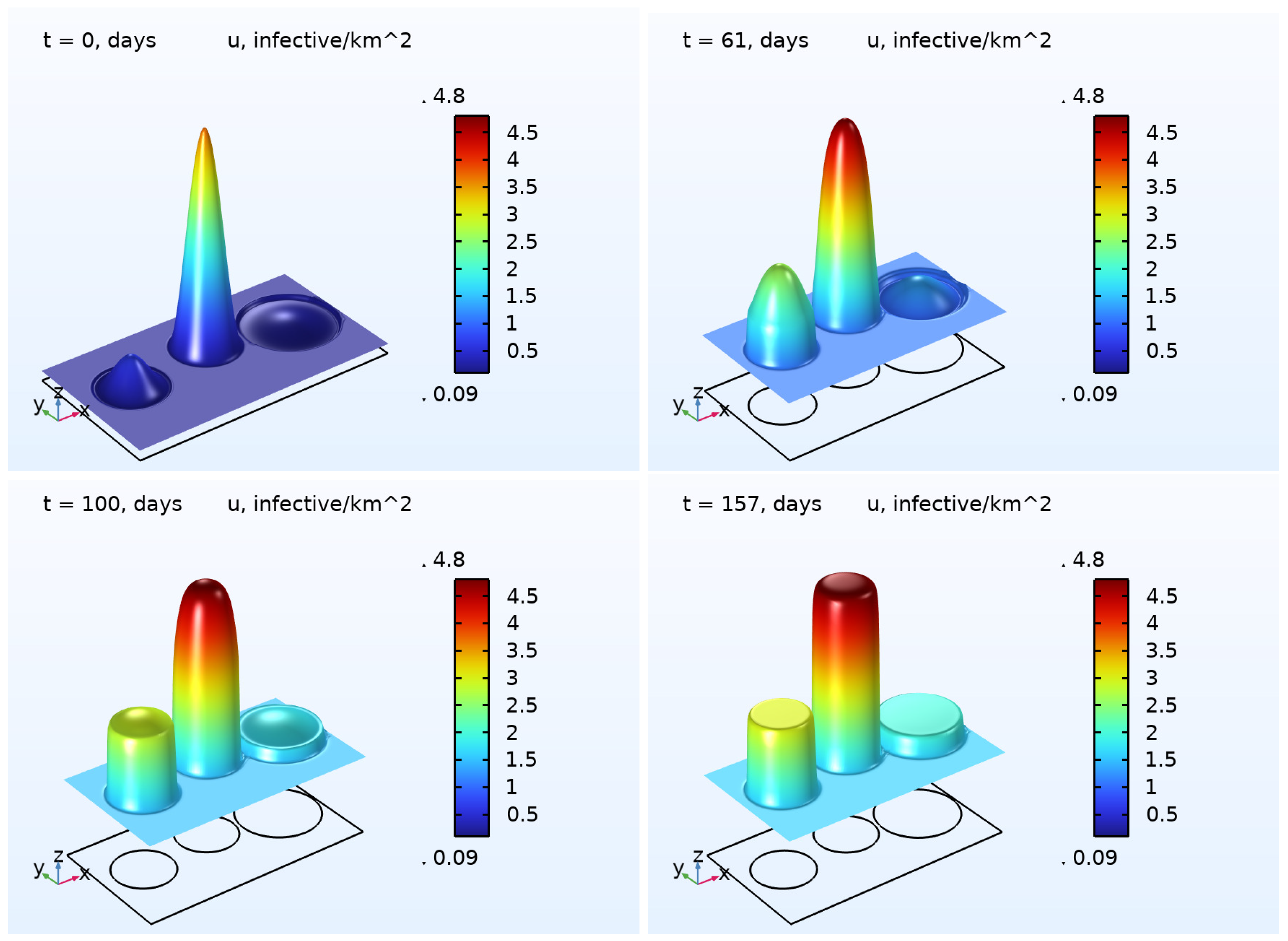
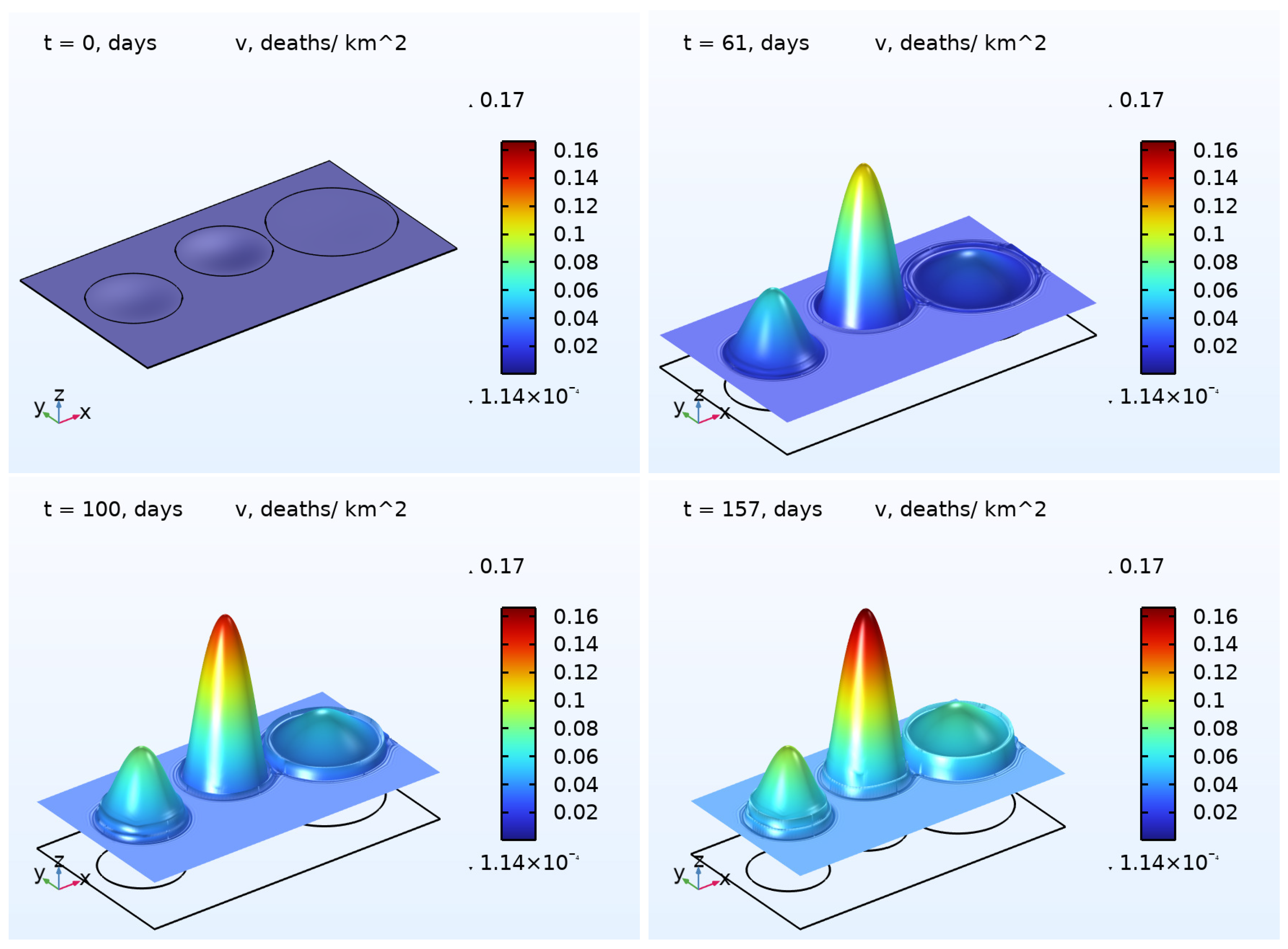
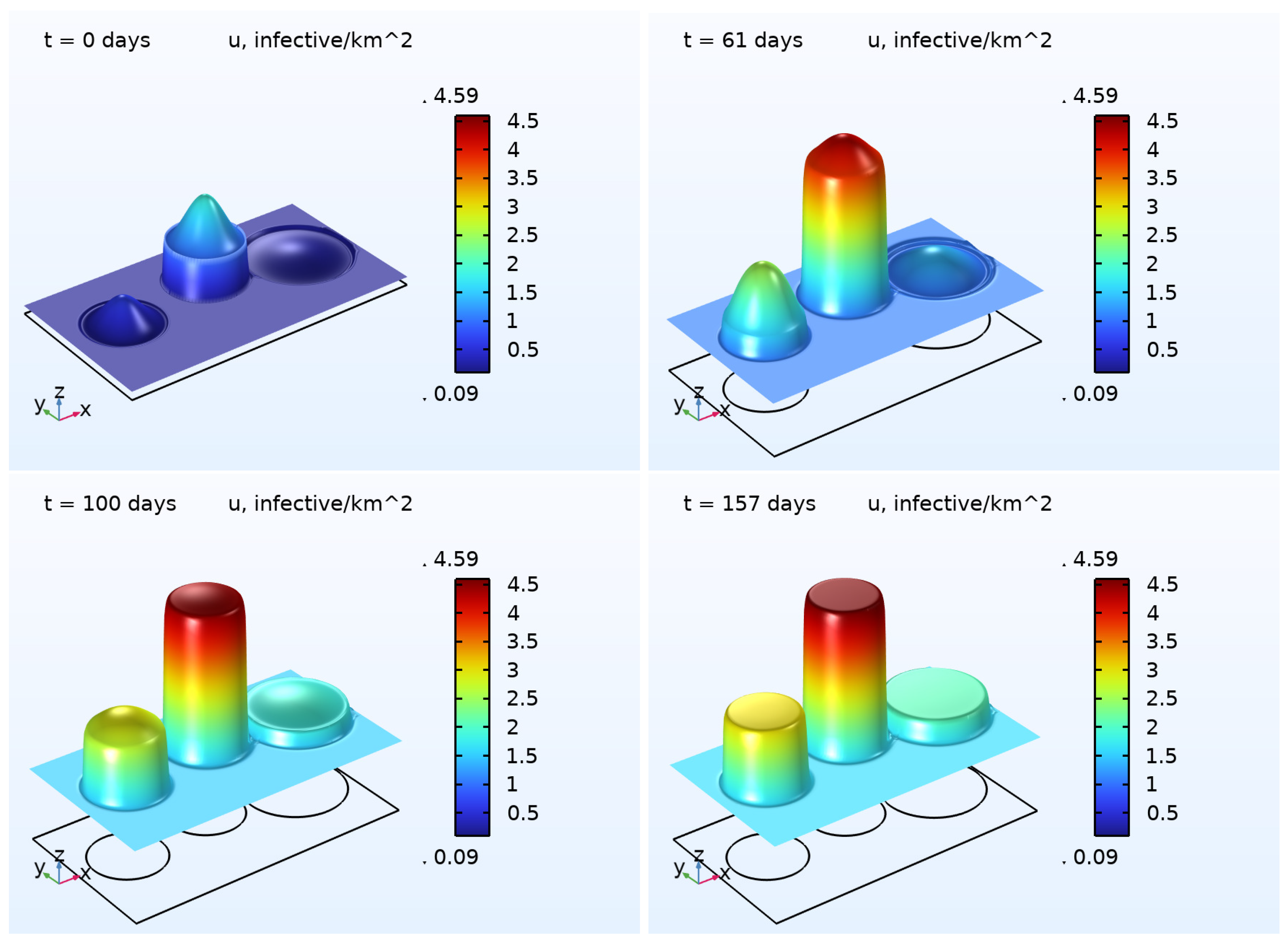
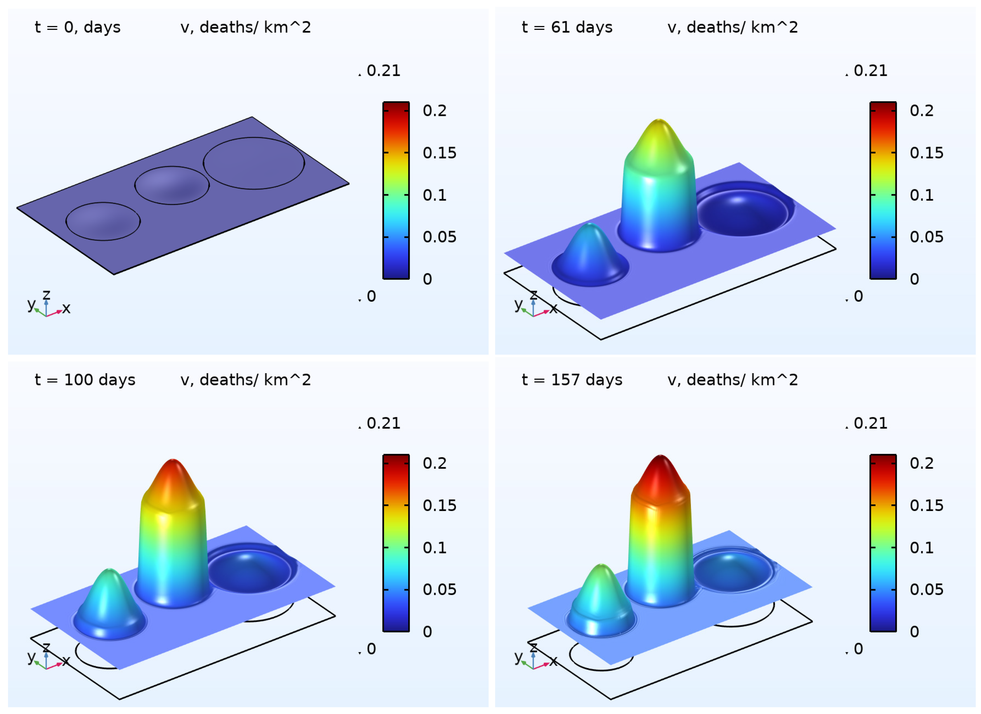
6) was numerically solved. The results are illustrated in
Figure 2 and
Figure 3, presenting the 3D plots for
and
. As one may easily note that, in the beginning of the pandemic wave, the densities of the COVID-19 cases were essentially inhomogeneous in all regions except the Rest region. At the end of the wave, the densities were close to some constants in each region. This effect is a result of the diffusion (random movement) of the infected persons. In contrast to the function
, the density of deaths
does not possess the property described above. We assume that such a difference occurs because of the zero diffusivity
.
Given the functions
and
, the total number of infection cases
and deaths
is calculated using Equation (
4). This was done for each region and for all of Ukraine as well. The numbers obtained were compared with the official data, which were adapted from the second wave, as described in
Section 4. In
Table 5 and
Table 6, the comparison is highlighted for the most important moments of the wave, the so-called tipping points. As one can conclude from
Table 5, in the case of the COVID-19 cases, the maximal inaccuracy is 7%, and that concerns the Rest region, while the minimal inaccuracy, only 2%, occurs in the West region. In
Table 6, the relevant comparison is presented for the number of deaths. The maximal inaccuracy is 22%, and that concerns the East region, while the minimal inaccuracy, 10%, is related to the West and Rest regions.
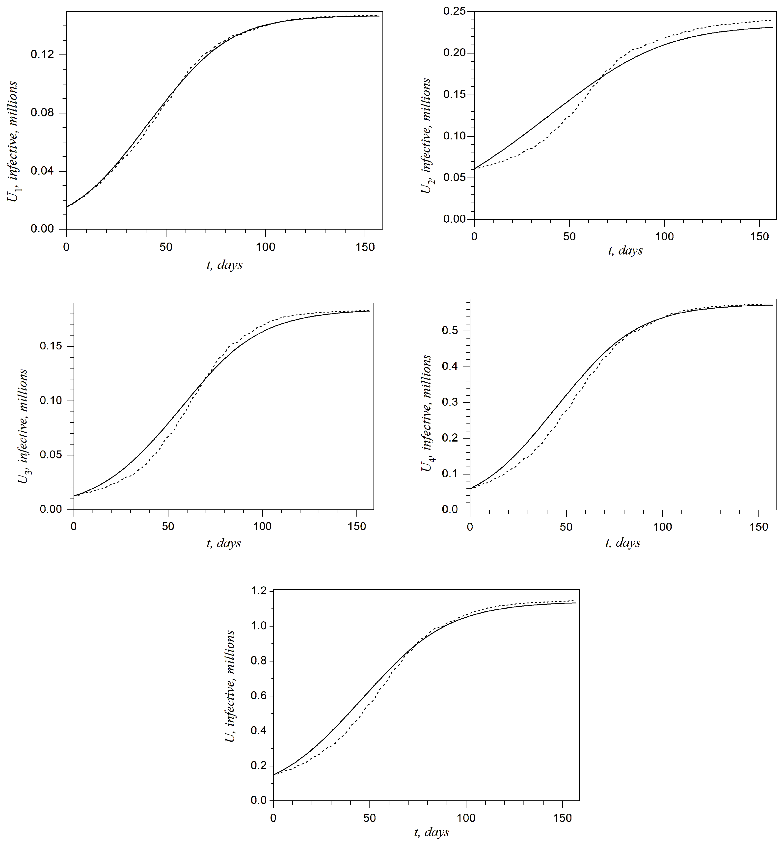
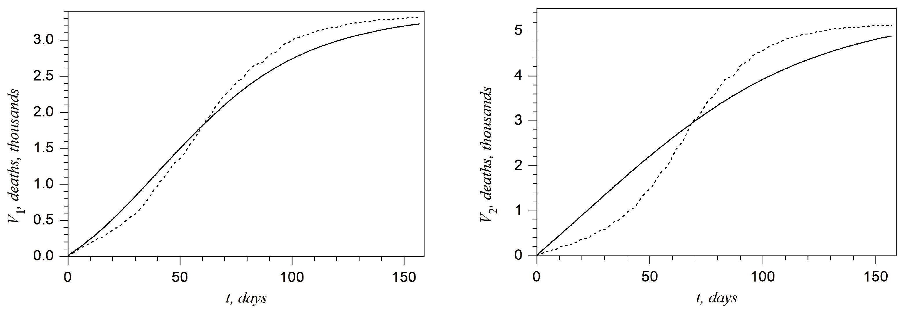
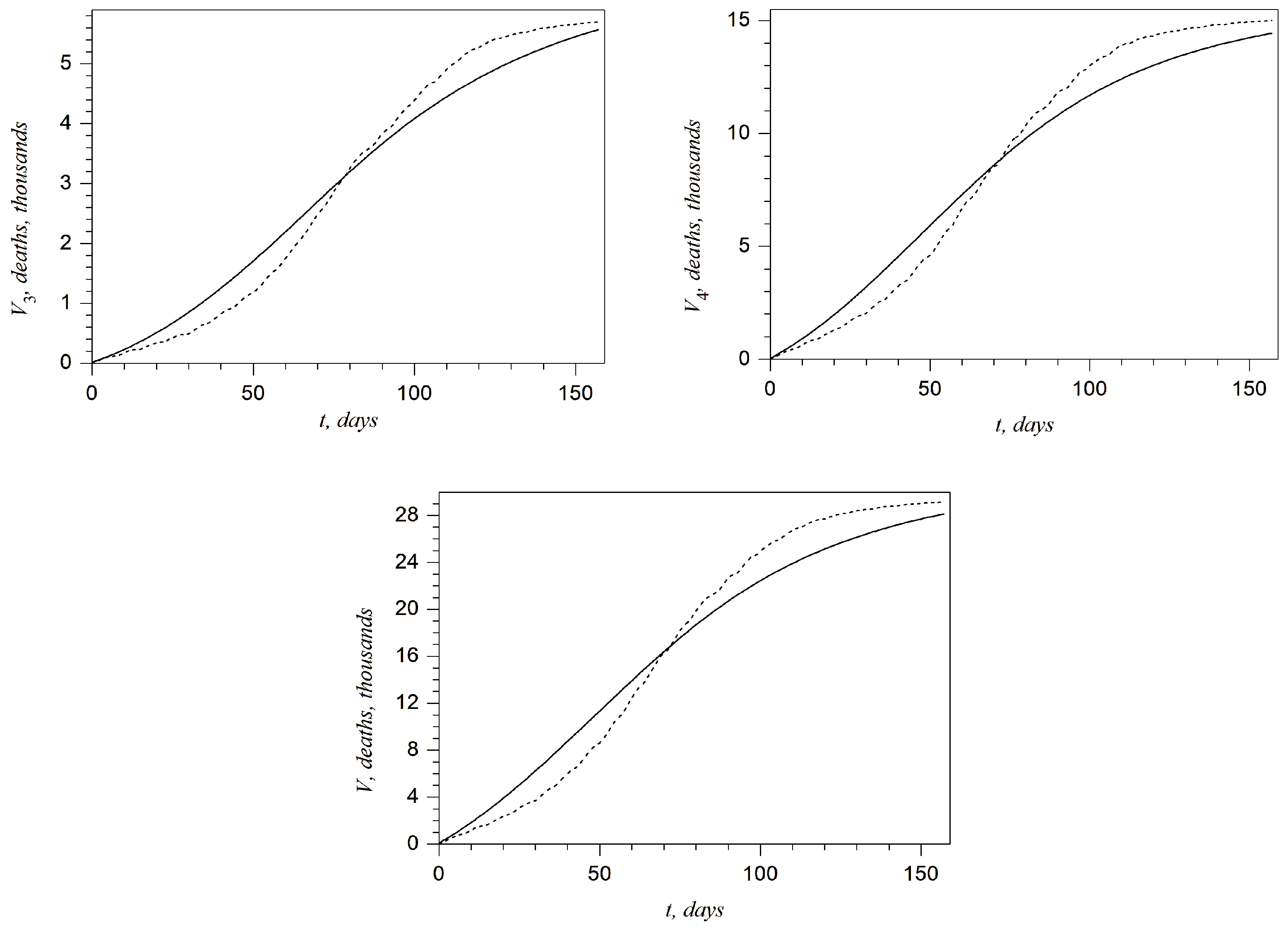
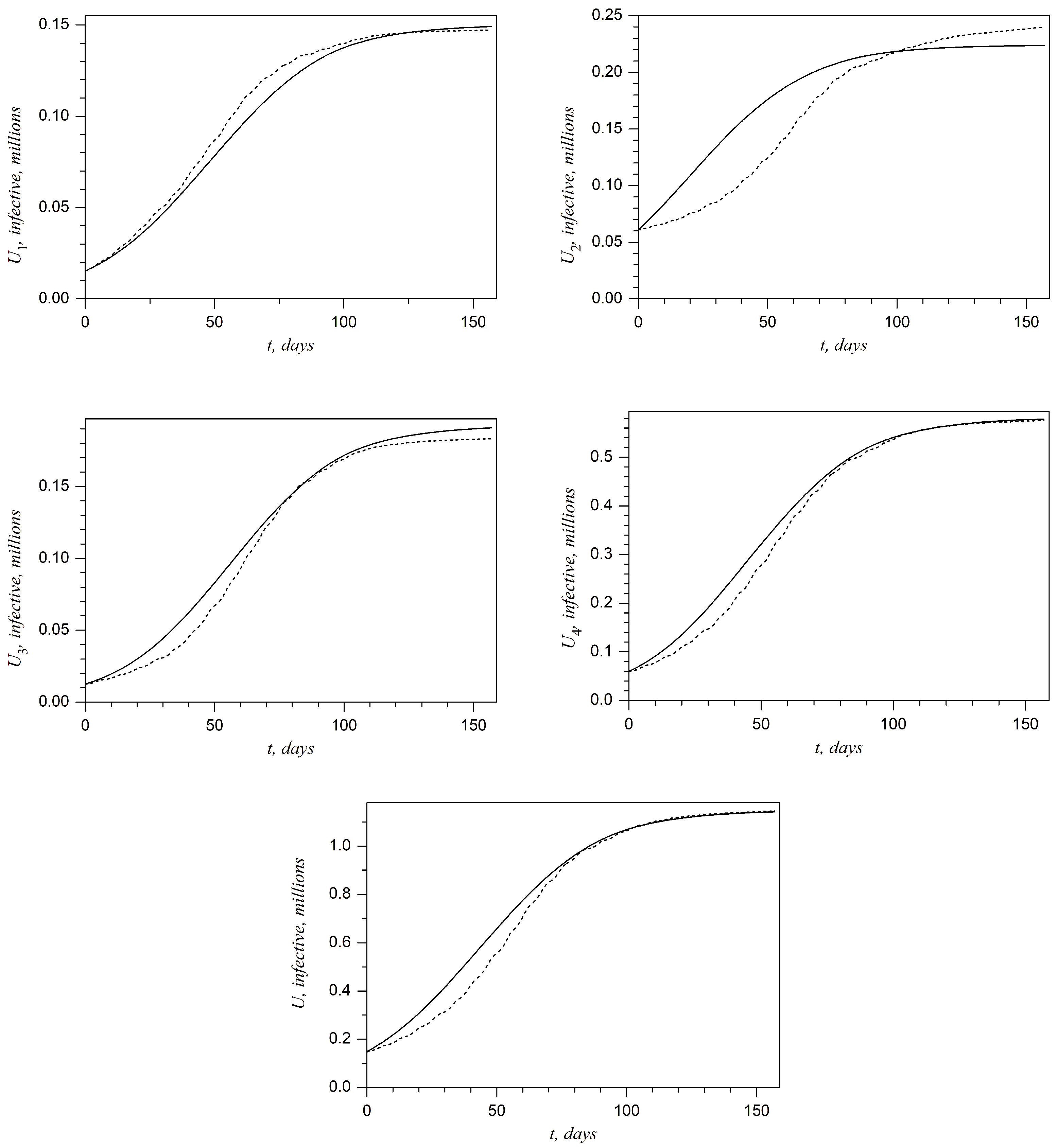
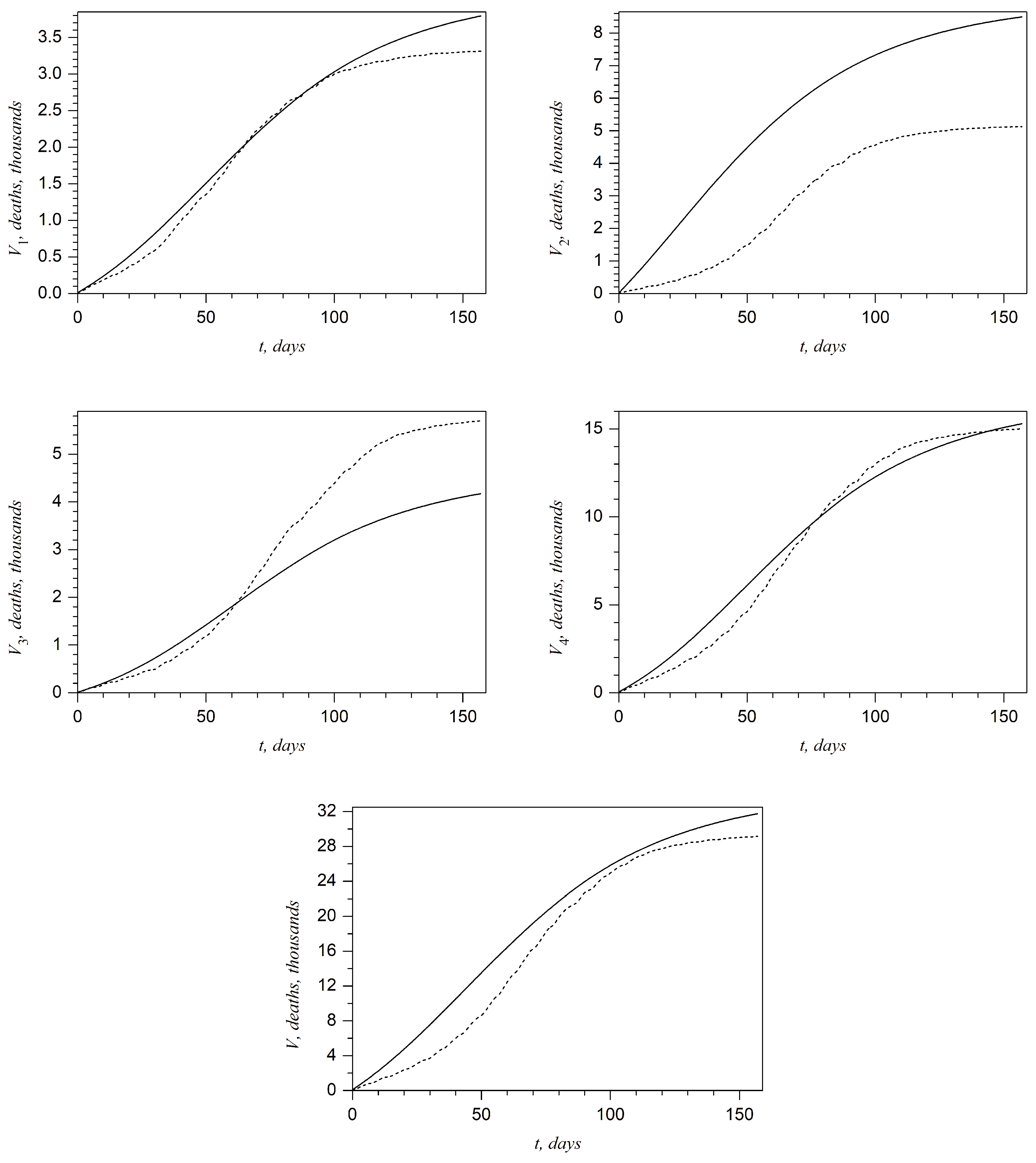
Plots presented in
Figure 4 and
Figure 5 show the above-described comparison at any day of the second wave in the West, Kyiv, East, and Rest regions and in all of Ukraine, respectively. It can be noted that the best accuracy is achieved for the West region. On the other hand, one can claim that the accuracy is not sufficient for the Kyiv region. This shortcoming will be discussed in the last section.
7. Results of Numerical Simulations with a Single Variable Parameter
in the Model
In the previous section, the parameters
, and
for each region were identified, and relevant numerical simulations were conducted and analyzed. Here, we fix three parameters for all regions and allow only the parameter
b to vary. The choice of
b follows from the analysis of
Table 4. In contrast to other parameters, values of
b are essentially different in the regions. In order to find average values for parameters
, and
, the population of each region was calculated using the official data [
29], and standard formulas based on weighting coefficients were applied. Thus, the average values are given by the formulas
where
, and
are taken from
Table 4;
has the following values
the number
corresponds to the region
i population; and
N is the population of Ukraine up to the date 1 February 2021. Using the formulas presented above, the following average parameters were obtained:
Having the correctly specified parameters (
16) and the parameters
= 1,
= 0.5 km
2/day, and
arising in the model, numerical simulations were conducted for a wide range of values of the parameter
b. As a result, the most appropriate values of
b for each region were identified as follows:
Given the correctly specified parameters (
16) and (
17) arising in the model, numerical simulations were conducted in order to solve the nonlinear BVP (
2), (
3), (
5) and (
6). The results are illustrated in
Figure 6 and
Figure 7, presenting the 3D plots for
and
. As one may easily note, the forms and time dynamics of the surfaces representing the densities
and
are very similar to those in
Figure 2 and
Figure 3. Thus, the simpler model, i.e., the above BVP with the single variable parameter
b can be used as well.
The plots presented in
Figure 8 and
Figure 9 show the comparison of the total number of COVID-19 cases and deaths during the second wave in the West, Kyiv, East, and Rest regions as well as in all of Ukraine with the official data. It can be noted that the accuracy related to the total number of COVID-19 cases is almost the same as in the case of four variable parameters (see the plots in
Figure 4 and
Figure 8). On the other hand, conclusions for the total number of deaths are not so optimistic. The best accuracy is achieved for the region Rest and for all of Ukraine. However, one can claim that the accuracy is essentially insufficient for the Kyiv and East regions (see the second and third plots in
Figure 9). This shortcoming is discussed below.
8. Discussion
In this study, the space distributed model of (
2), (
3), (
5) and (
6) proposed earlier in [
16,
17] was adopted for modeling the second wave of the COVID-19 pandemic in Ukraine. Because the geometrical shape of Ukraine is very complicated, the shape of Ukraine (excluding the temporarily occupied territories in 2014) was approximated by a rectangle that consists of four different regions. Three of them have the form of rings, while the fourth region occupies the rest of the rectangle. It was shown that the governing equations of the model should be generalized (see Equation (
14)) in order to obtain the results that correspond to the official data of the COVID-19 cases and deaths published in [
26,
27].
A wide range of numerical simulations was conducted with the aim of obtaining the correctly specified parameters arising in the model. Having done this, the total densities of the COVID-19 cases
u and deaths
v during the second wave were obtained by numerical simulations. At the final stage, the number of COVID-19 cases
U and deaths
V in each region was calculated using the densities
u and
v. Comparison with the official data shows that the model works very well if four parameters (see
Table 4) are adopted for the relevant region. If only parameter
b is specified for each region, while other parameters take average values, then the result of the comparison is not so optimistic. In particular, the obtained number of deaths essentially deviates from the official data.
In this work, in contrast to many works [
2,
3,
5,
6,
8,
9,
11,
12,
15] in which mathematical models are applied to COVID-19 spread in specific regions of several countries, the space distributed model developed by the authors is applied to the entire country of Ukraine with a large area and population. To the best of our knowledge, this study is the first in which the COVID-19 pandemic in Ukraine was studied by a model involving partial differential equations. Moreover, the model is not a generalization (modification) of well-known models; therefore, it is important to demonstrate its applicability.
It should be pointed out that the mathematical model was solved under essential simplifications and assumptions. Firstly, the real geometrical shape of Ukraine is more complicated than the rectangle presented in
Figure 1; secondly, Ukraine is a large country consisting of 25 administrative regions (without TOTs). Thus, the results of numerical simulations will be closer to the official data provided a proper approximation of the country’s geometry and a larger number of regions are used.
We also foresee that the parameter
in the first governing equation (see Equation (
2)) plays an essential role. Although the choice
seems to be reasonable, it was shown in [
16] that the value
works better for several European countries. Thus, one may expect that the best choice can be
. Finally, one open problem remains concerning the diffusivities
and
. Our choice was based only on numerical simulations and the plausible assumption
; however, some analytical estimations are needed in order to estimate
and
. We are going to study the issues highlighted above in a forthcoming paper.
