
Improved Generalized-Pinball-Loss-Based Laplacian Twin Support Vector Machine for Data Classification


Abstract
1. Introduction
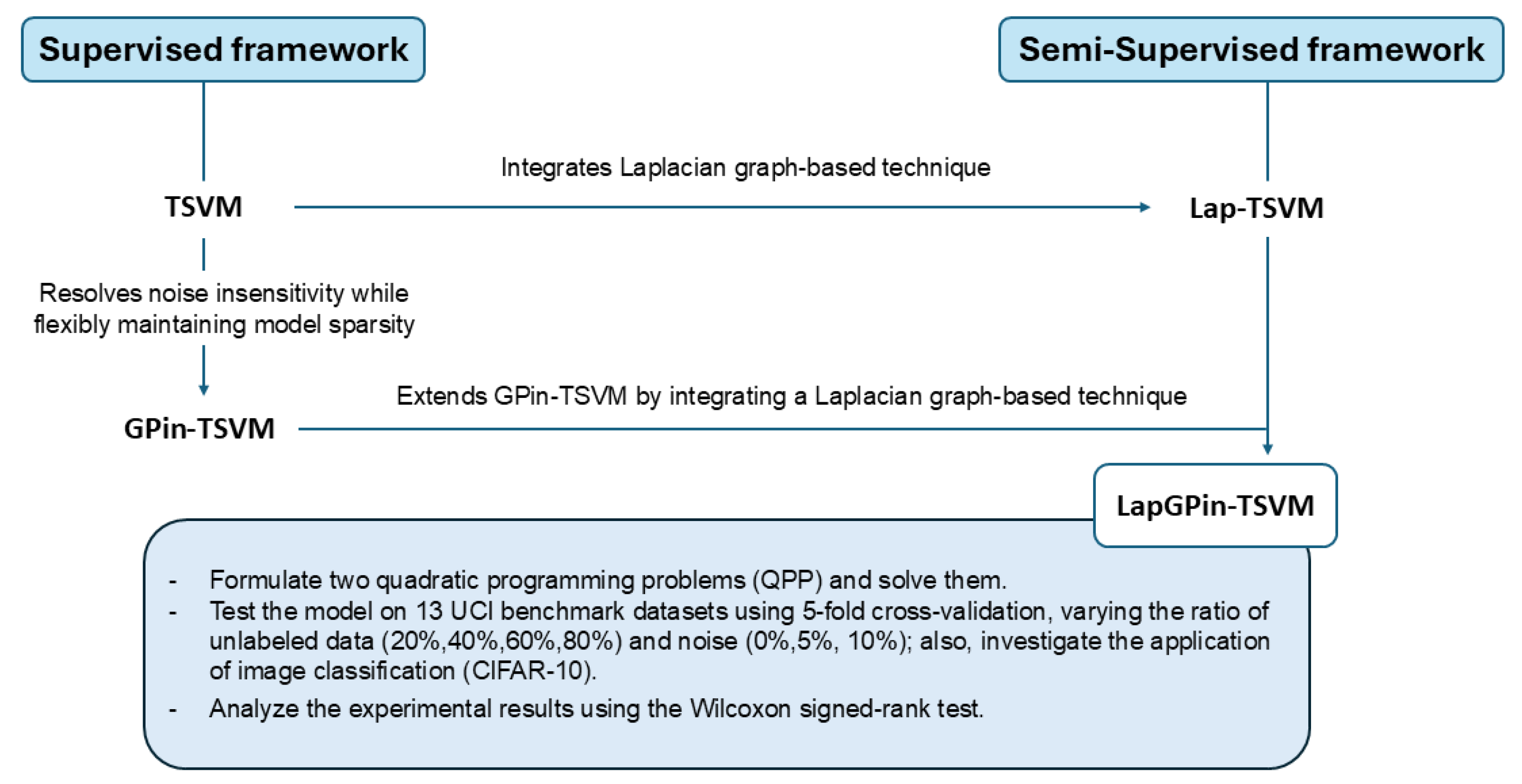
- We combine the twin support vector machine based on the generalized pinball loss (GPin-TSVM) with the Laplacian technique, introducing a novel semi-supervised framework named LapGPin-TSVM. Additionally, we demonstrate noise insensitivity along with a corresponding analysis.
- We evaluate the efficacy of our model through experiments on the UCI dataset, using various ratios of unlabeled data and noise, and compare the results with three state-of-the-art models. Moreover, we also investigate the application of our approach to image classification.
- To analyze the performance of LapGPin-TSVM, we employ the win/tie/loss method, average rank, and use the Wilcoxon signed-rank test to better describe the effectiveness of our proposed method.
2. Preliminaries
2.1. Twin Support Vector Machine (TSVM)
2.2. Twin Support Vector Machine with Generalized Pinball Loss (GPin-TSVM)
2.3. Laplacian Twin Support Vector Machine
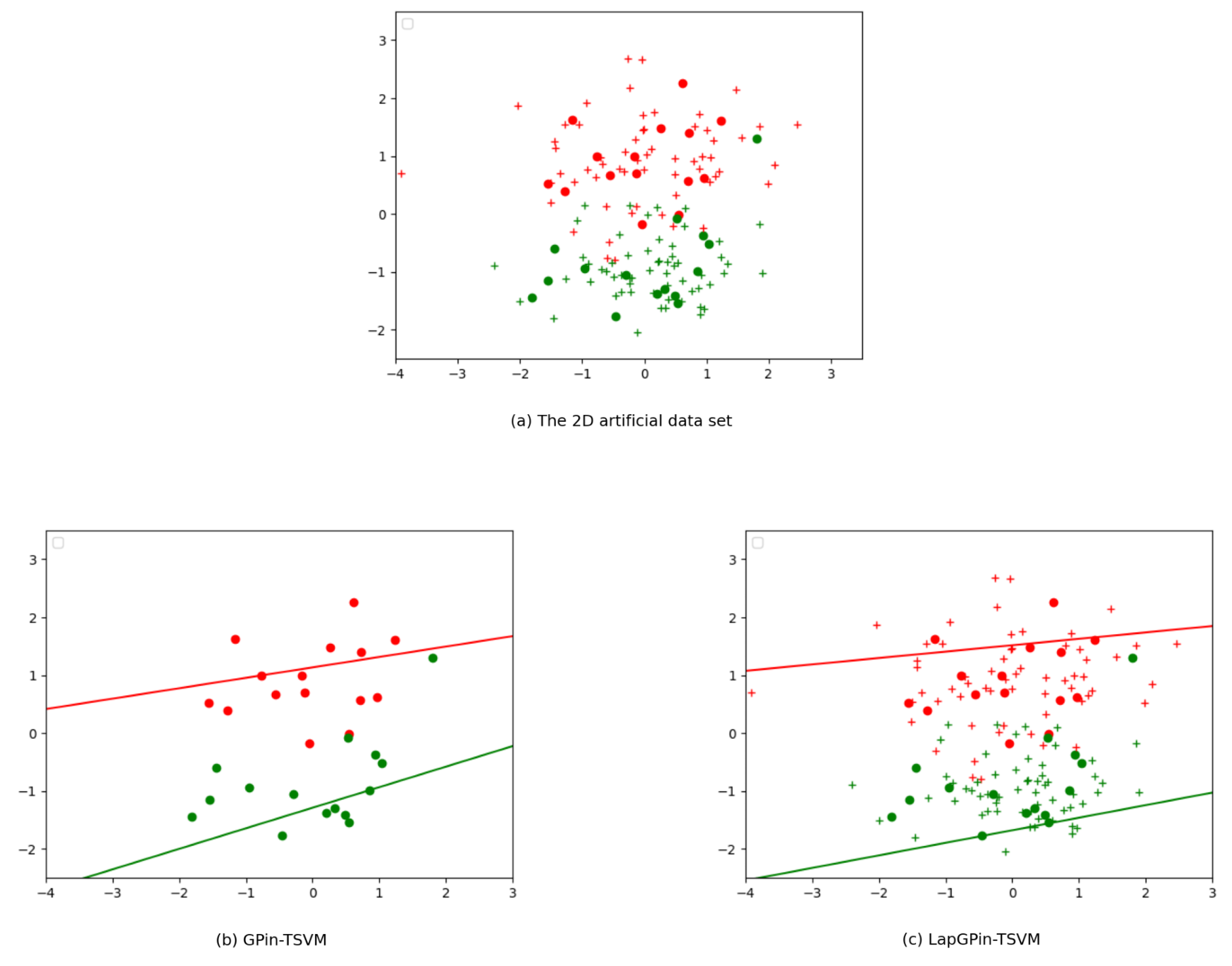
3. Proposed Work
3.1. Primal Problem
3.2. Dual Problem
| Algorithm 1 LapGPin-TSVM |
|
3.3. Property of the Lap-GPTSVM
Noise Insensitivity
4. Comparison of the Models
4.1. LapGPin-TSVM vs. GPin-TSVM
4.2. LapGPin-TSVM vs. Lap-TSVM
4.3. LapGPin-TSVM vs. Lap-PTSVM
5. Numerical Experiments
5.1. Evaluation Metrics
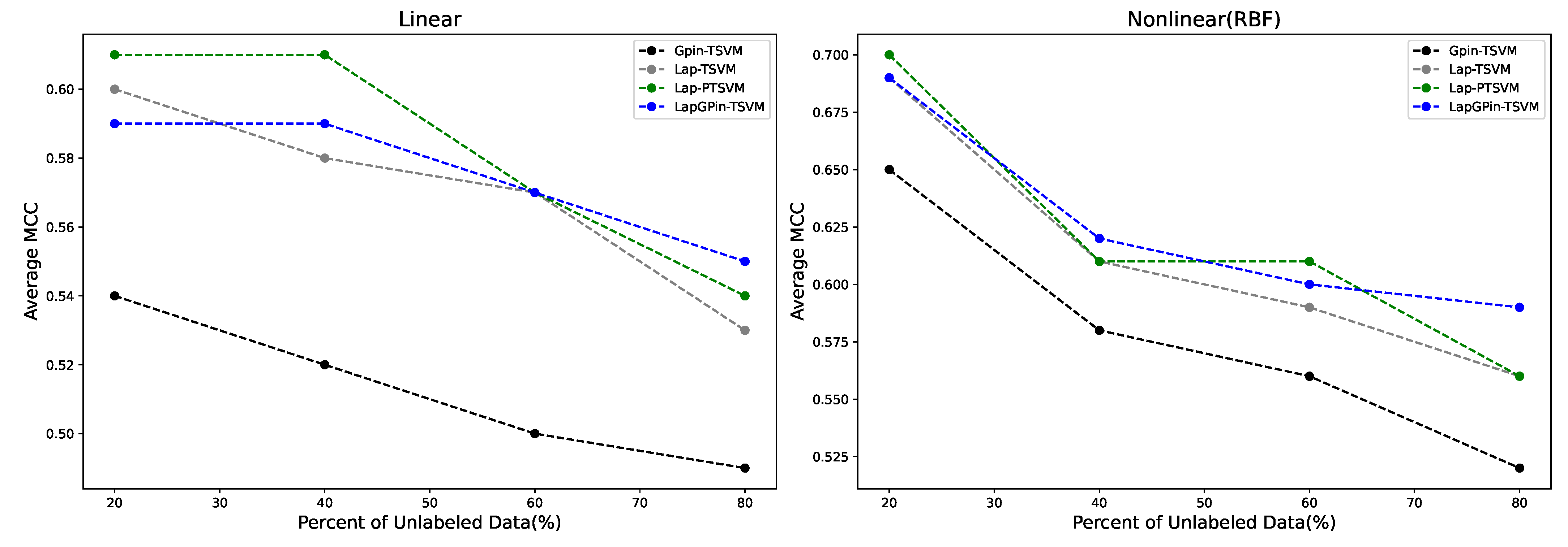
5.2. Variation in Ratio of Unlabeled Data
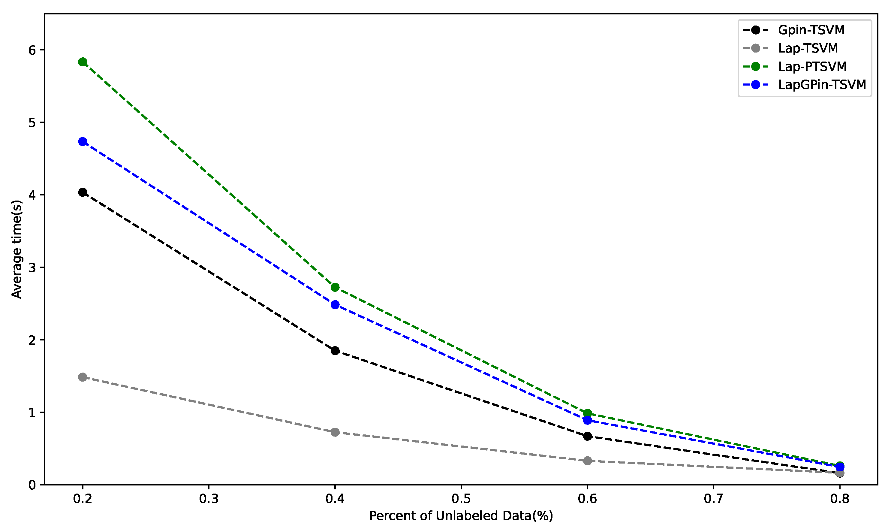
Computational Efficiency of Model
5.3. Ablation Study
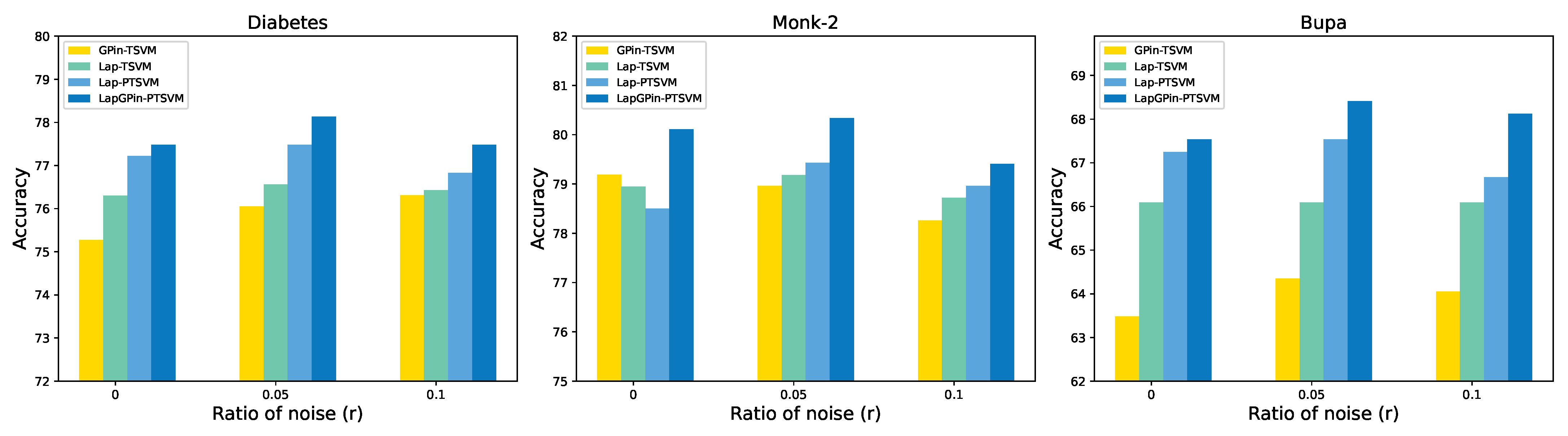
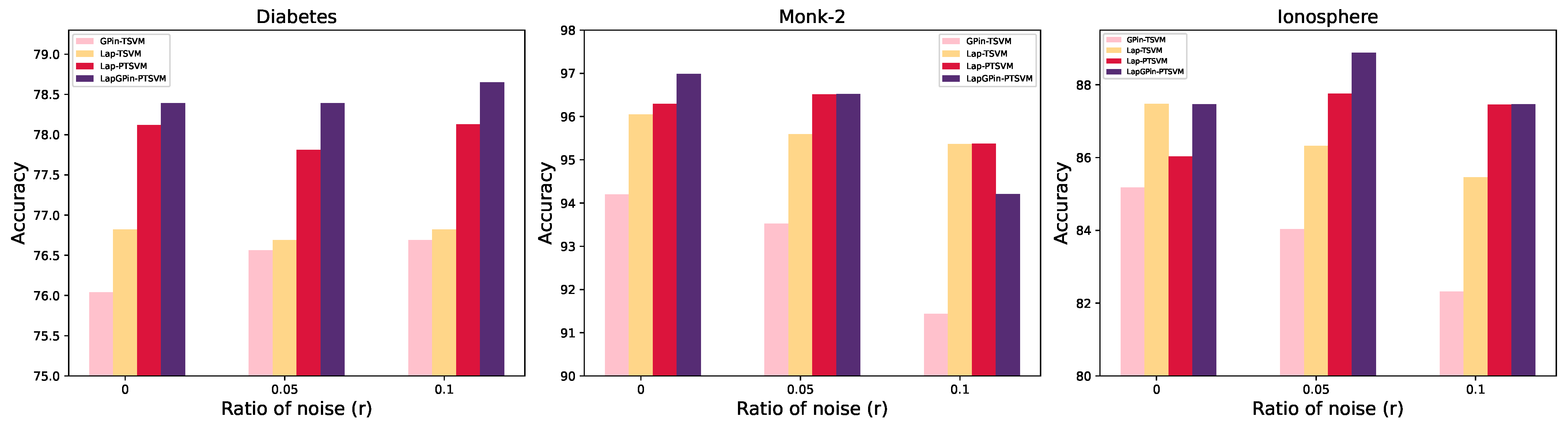
5.4. Variation in Ratio of Noise
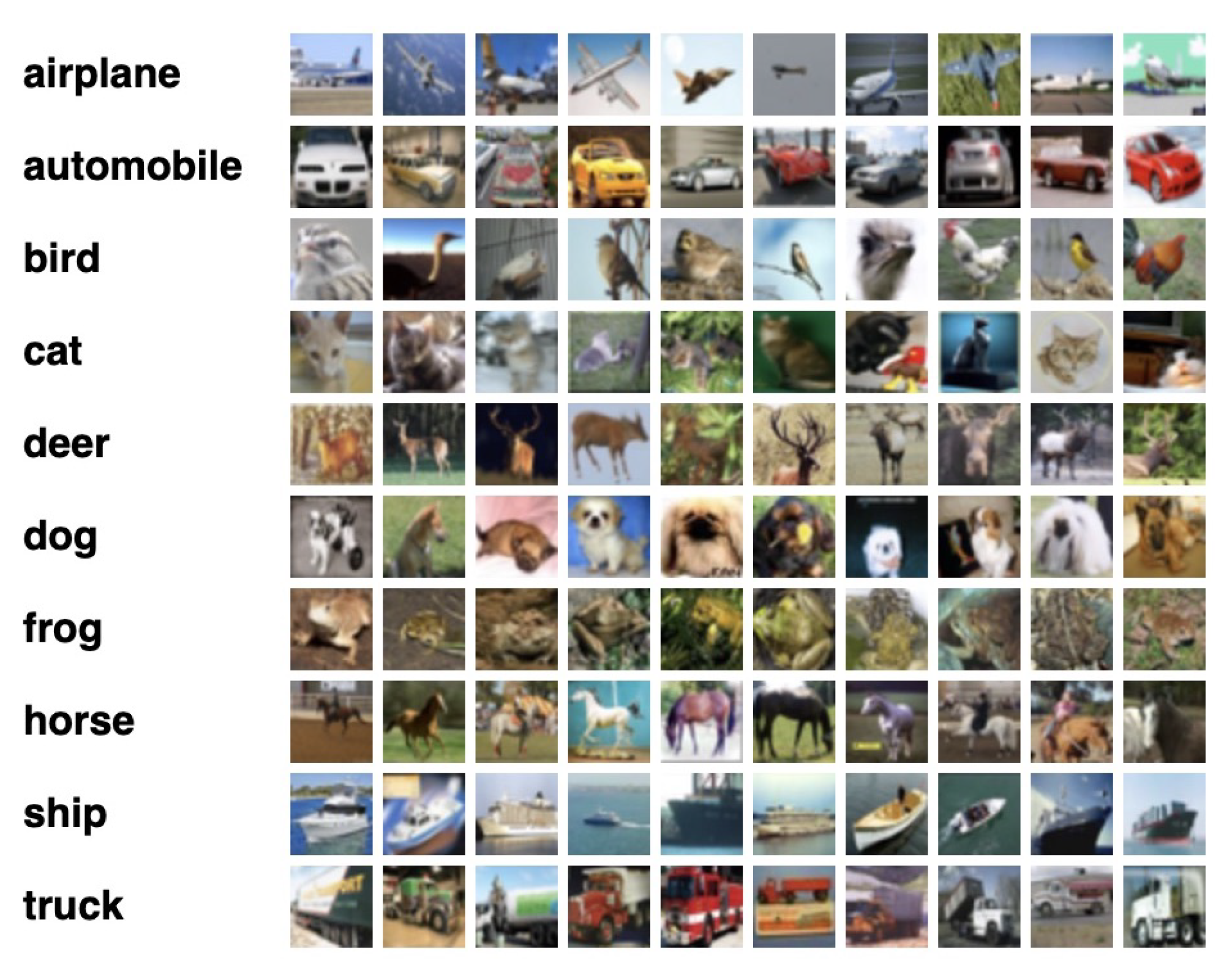
5.5. Experiment on an Image Dataset
6. Discussion
7. Conclusions
Author Contributions
Funding
Data Availability Statement
Acknowledgments
Conflicts of Interest
References
- Christmann, A.; Steinwart, I. Support Vector Machines; Springer: Berlin/Heidelberg, Germany, 2008. [Google Scholar]
- Jayadeva; Khemchandani, R.; Chandra, S. Twin Support Vector Machines for Pattern Classification. IEEE Trans. Pattern Anal. Mach. Intell. 2007, 29, 905–910. [Google Scholar] [CrossRef] [PubMed]
- Kumar, M.A.; Gopal, M. Least Squares Twin Support Vector Machines for Pattern Classification. Expert Syst. Appl. 2009, 36, 7535–7543. [Google Scholar] [CrossRef]
- Mei, B.; Xu, Y. Multi-task Least Squares Twin Support Vector Machine for Classification. Neurocomputing 2019, 338, 26–33. [Google Scholar] [CrossRef]
- Rastogi, R.; Sharma, S.; Chandra, S. Robust parametric twin support vector machine for pattern classification. Neural Process. Lett. 2018, 47, 293–323. [Google Scholar] [CrossRef]
- Xie, X.; Sun, F.; Qian, J.; Guo, L.; Zhang, R.; Ye, X.; Wang, Z. Laplacian Lp Norm Least Squares Twin Support Vector Machine. Pattern Recognit. 2023, 136, 109192. [Google Scholar] [CrossRef]
- Li, Y.; Sun, H. Safe Sample Screening for Robust Twin Support Vector Machine. Appl. Intell. 2023, 53, 20059–20075. [Google Scholar] [CrossRef]
- Si, Q.; Yang, Z.; Ye, J. Symmetric LINEX Loss Twin Support Vector Machine for Robust Classification and Its Fast Iterative Algorithm. Neural Netw. 2023, 168, 143–160. [Google Scholar] [CrossRef]
- Gupta, U.; Gupta, D. Least Squares Structural Twin Bounded Support Vector Machine on Class Scatter. Appl. Intell. 2023, 53, 15321–15351. [Google Scholar] [CrossRef]
- Tanveer, M.; Rajani, T.; Rastogi, R.; Shao, Y.H.; Ganaie, M.A. Comprehensive Review on Twin Support Vector Machines. Ann. Oper. Res. 2022, 1–46. [Google Scholar] [CrossRef]
- Rezvani, S.; Wang, X.; Pourpanah, F. Intuitionistic Fuzzy Twin Support Vector Machines. IEEE Trans. Fuzzy Syst. 2019, 27, 2140–2151. [Google Scholar] [CrossRef]
- Xu, Y.; Yang, Z.; Pan, X. A Novel Twin Support-Vector Machine with Pinball Loss. IEEE Trans. Neural Netw. Learn. Syst. 2016, 28, 359–370. [Google Scholar] [CrossRef] [PubMed]
- Tanveer, M.; Sharma, A.; Suganthan, P.N. General Twin Support Vector Machine with Pinball Loss Function. Inf. Sci. 2019, 494, 311–327. [Google Scholar] [CrossRef]
- Tanveer, M.; Tiwari, A.; Choudhary, R.; Jalan, S. Sparse Pinball Twin Support Vector Machines. Appl. Soft Comput. 2019, 78, 164–175. [Google Scholar] [CrossRef]
- Rastogi, R.; Pal, A.; Chandra, S. Generalized Pinball Loss SVMs. Neurocomputing 2018, 322, 151–165. [Google Scholar] [CrossRef]
- Panup, W.; Ratipapongton, W.; Wangkeeree, R. A Novel Twin Support Vector Machine with Generalized Pinball Loss Function for Pattern Classification. Symmetry 2022, 14, 289. [Google Scholar] [CrossRef]
- Alloghani, M.; Al-Jumeily, D.; Mustafina, J.; Hussain, A.; Aljaaf, A.J. A Systematic Review on Supervised and Unsupervised Machine Learning Algorithms for Data Science. In Supervised and Unsupervised Learning for Data Science; Springer Nature: Berlin, Germany, 2020; pp. 3–21. [Google Scholar]
- Reddy, Y.C.A.P.; Viswanath, P.; Reddy, B.E. Semi-supervised Learning: A Brief Review. Int. J. Eng. Technol. 2018, 7, 81. [Google Scholar] [CrossRef]
- Zhang, W.; Li, Z.; Li, G.; Zhuang, P.; Hou, G.; Zhang, Q.; Li, C. Gacnet: Generate adversarial-driven cross-aware network for hyperspectral wheat variety identification. IEEE Trans. Geosci. Remote Sens. 2023, 62, 5503314. [Google Scholar] [CrossRef]
- Zhang, W.; Zhao, W.; Li, J.; Zhuang, P.; Sun, H.; Xu, Y.; Li, C. CVANet: Cascaded visual attention network for single image super-resolution. Neural Netw. 2024, 170, 622–634. [Google Scholar] [CrossRef]
- Zhang, W.; Chen, G.; Zhuang, P.; Zhao, W.; Zhou, L. CATNet: Cascaded attention transformer network for marine species image classification. Expert Syst. Appl. 2024, 256, 124932. [Google Scholar] [CrossRef]
- Zhang, Q.; Lee, F.; Wang, Y.g.; Ding, D.; Yao, W.; Chen, L.; Chen, Q. An joint end-to-end framework for learning with noisy labels. Appl. Soft Comput. 2021, 108, 107426. [Google Scholar] [CrossRef]
- Zhang, Q.; Zhu, Y.; Yang, M.; Jin, G.; Zhu, Y.; Chen, Q. Cross-to-merge training with class balance strategy for learning with noisy labels. Expert Syst. Appl. 2024, 249, 123846. [Google Scholar] [CrossRef]
- Zhang, Q.; Jin, G.; Zhu, Y.; Wei, H.; Chen, Q. BPT-PLR: A Balanced Partitioning and Training Framework with Pseudo-Label Relaxed Contrastive Loss for Noisy Label Learning. Entropy 2024, 26, 589. [Google Scholar] [CrossRef] [PubMed]
- Qi, Z.; Tian, Y.; Shi, Y. Laplacian Twin Support Vector Machine for Semi-supervised Classification. Neural Netw. 2012, 35, 46–53. [Google Scholar] [CrossRef] [PubMed]
- Merris, R. Laplacian Graph Eigenvectors. Linear Algebra Its Appl. 1998, 278, 221–236. [Google Scholar] [CrossRef]
- Chen, W.J.; Shao, Y.H.; Deng, N.Y.; Feng, Z.L. Laplacian Least Squares Twin Support Vector Machine for Semi-supervised Classification. Neurocomputing 2014, 145, 465–476. [Google Scholar] [CrossRef]
- Damminsed, V.; Panup, W.; Wangkeeree, R. Laplacian Twin Support Vector Machine with Pinball Loss for Semi-supervised Classification. IEEE Access 2023, 11, 31399–31416. [Google Scholar] [CrossRef]
- Huang, X.; Shi, L.; Suykens, J.A.K. Support Vector Machine Classifier with Pinball Loss. IEEE Trans. Pattern Anal. Mach. Intell. 2013, 36, 984–997. [Google Scholar] [CrossRef]
- Meyes, R.; Lu, M.; de Puiseau, C.W.; Meisen, T. Ablation studies in artificial neural networks. arXiv 2019, arXiv:1901.08644. [Google Scholar]
- García, S.; Fernández, A.; Luengo, J.; Herrera, F. Advanced Nonparametric Tests for Multiple Comparisons in the Design of Experiments in Computational Intelligence and Data Mining: Experimental Analysis of Power. Inf. Sci. 2010, 180, 2044–2064. [Google Scholar] [CrossRef]
- Demšar, J. Statistical Comparisons of Classifiers over Multiple Data Sets. J. Mach. Learn. Res. 2006, 7, 1–30. [Google Scholar]
- Krizhevsky, A.; Hinton, G. Learning Multiple Layers of Features from Tiny Images; Computer Science University of Toronto: Toronto, ON, Canada, 2009. [Google Scholar]


| Datasets | No. of Samples | No. of Features |
|---|---|---|
| Ionosphere | 351 | 33 |
| Bupa | 345 | 6 |
| Fertility | 100 | 10 |
| Pima | 768 | 8 |
| Banknote | 1372 | 4 |
| Monk-2 | 432 | 7 |
| Sonar | 208 | 60 |
| Diabetes | 769 | 9 |
| Spambase | 4601 | 57 |
| WDBC | 569 | 30 |
| Australian | 690 | 14 |
| Heart | 303 | 13 |
| Specf heart | 267 | 22 |
| GPin-TSVM | Lap-TSVM | Lap-PTSVM | LapGPin-TSVM | ||
|---|---|---|---|---|---|
| Datasets | Acc (%) | Acc (%) | Acc (%) | Acc (%) | |
| MCC | MCC | MCC | MCC | ||
| Time (s) | Time (s) | Time (s) | Time (s) | ||
| Fertility | Linear | 88.00 ± 5.10 | 88.00 ± 5.10 | 88.00 ± 5.10 | 88.00 ± 5.10 |
| 0.0500 | 0.000 | 0.000 | 0.000 | ||
| 0.0352 | 0.0361 | 0.0397 | 0.0404 | ||
| RBF | 88.00 ± 4.00 | 88.00 ± 4.00 | 88.00 ± 4.00 | 88.00 ± 4.00 | |
| 0.0000 | 0.000 | 0.000 | 0.000 | ||
| 0.0469 | 0.0421 | 0.0521 | 0.0570 | ||
| Banknote | Linear | 93.88 ± 1.97 | 98.98 ± 0.63 | 97.52 ± 1.43 | 98.03 ± 0.94 |
| 0.8804 | 0.9793 | 0.9516 | 0.9607 | ||
| 2.1492 | 0.6919 | 0.9516 | 0.9607 | ||
| RBF | 100.00 ± 0.00 | 99.78 ± 0.18 | 99.85 ± 0.29 | 100.00 ± 0.00 | |
| 1.000 | 0.9956 | 0.9971 | 1.000 | ||
| 2.2177 | 0.6225 | 2.6625 | 2.1435 | ||
| Bupa | Linear | 60.00 ± 3.85 | 68.41 ± 4.80 | 67.53 ± 3.50 | 67.25 ± 3.73 |
| 0.8804 | 0.9793 | 0.9516 | 0.9607 | ||
| 2.1492 | 0.6919 | 0.9516 | 0.9607 | ||
| RBF | 68.69 ± 7.25 | 66.67 ± 4.80 | 67.53 ± 3.50 | 67.25 ± 3.73 | |
| 0.8804 | 0.9793 | 0.9516 | 0.9607 | ||
| 2.1492 | 0.6919 | 0.9516 | 0.9607 | ||
| Ionosphere | Linear | 81.48 ± 3.75 | 88.03 ± 2.51 | 87.74 ± 2.35 | 90.88 ± 2.66 |
| 0.6207 | 0.7419 | 0.7365 | 0.8040 | ||
| 0.3662 | 0.1751 | 0.1499 | 0.1080 | ||
| RBF | 89.19 ± 3.94 | 92.89 ± 4.21 | 91.18 ± 3.11 | 91.18 ± 2.74 | |
| 0.7709 | 0.8443 | 0.8065 | 0.8068 | ||
| 0.1506 | 0.0732 | 0.1158 | 0.1205 | ||
| Monk-2 | Linear | 79.17 ± 3.74 | 83.81 ± 1.98 | 86.35 ± 2.04 | 80.55 ± 2.25 |
| 0.5914 | 0.6769 | 0.7278 | 0.6264 | ||
| 0.1253 | 0.0956 | 0.1670 | 0.1221 | ||
| RBF | 96.29 ± 3.71 | 97.22 ± 3.33 | 97.22 ± 3.33 | 97.22 ± 3.33 | |
| 0.9272 | 0.9464 | 0.9464 | 0.9464 | ||
| 0.1726 | 0.0986 | 0.1809 | 0.1586 | ||
| Pima | Linear | 68.36 ± 2.76 | 75.39 ± 1.41 | 75.39 ± 1.41 | 76.95 ± 1.06 |
| 0.2343 | 0.4251 | 0.4251 | 0.4687 | ||
| 0.5448 | 0.1411 | 0.6538 | 0.4987 | ||
| RBF | 72.67 ± 4.82 | 75.79 ± 3.06 | 79.97 ± 4.15 | 76.05 ± 4.01 | |
| 0.3663 | 0.4424 | 0.4716 | 0.4499 | ||
| 0.5341 | 0.1874 | 0.4813 | 0.5510 | ||
| Sonar | Linear | 75.45 ± 9.58 | 77.86 ± 6.07 | 78.36 ± 6.25 | 77.86 ± 6.54 |
| 0.5380 | 0.5585 | 0.5723 | 0.5605 | ||
| 0.0632 | 0.0688 | 0.0710 | 0.0704 | ||
| RBF | 75.45 ± 3.08 | 77.92 ± 6.17 | 79.83 ± 2.28 | 77.91 ± 4.79 | |
| 0.5185 | 0.5605 | 0.5955 | 0.5642 | ||
| 0.0552 | 0.0546 | 0.0779 | 0.0661 | ||
| Diabetes | Linear | 75.39 ± 1.62 | 74.48 ± 2.19 | 77.73 ± 1.95 | 76.82 ± 2.11 |
| 0.4350 | 0.4093 | 0.4928 | 0.4722 | ||
| 0.4728 | 0.1441 | 0.6376 | 0.5980 | ||
| RBF | 75.77 ± 2.03 | 76.43 ± 1.47 | 76.82 ± 1.63 | 76.95 ± 1.13 | |
| 0.4433 | 0.4611 | 0.4715 | 0.4744 | ||
| 0.5273 | 0.2047 | 0.6880 | 0.5473 | ||
| Spambase | Linear | 84.08 ± 1.01 | 90.45 ± 0.91 | 91.32 ± 1.11 | 91.12 ± 0.95 |
| 0.7106 | 0.8000 | 0.8177 | 0.8135 | ||
| 50.0703 | 16.4100 | 61.5567 | 42.6016 | ||
| RBF | 88.41 ± 0.97 | 90.30 ± 1.09 | 91.28 ± 0.57 | 91.41 ± 0.51 | |
| 0.7569 | 0.7971 | 0.8186 | 0.8194 | ||
| 41.5564 | 17.3560 | 79.4900 | 70.7805 | ||
| WDBC | linear | 88.93 ± 1.17 | 92.96 ± 1.86 | 94.90 ± 1.52 | 95.78 ± 1.41 |
| 0.7729 | 0.8594 | 0.8927 | 0.9106 | ||
| 0.2742 | 0.1037 | 0.3075 | 0.2995 | ||
| RBF | 93.15 ± 1.02 | 95.26 ± 2.57 | 95.26 ± 2.63 | 95.43 ± 2.79 | |
| 0.8597 | 0.8992 | 0.8991 | 0.9051 | ||
| 0.2595 | 0.1216 | 0.3249 | 0.3304 | ||
| Australian | linear | 64.35 ± 3.79 | 85.65 ± 4.21 | 85.94 ± 4.36 | 86.09 ± 3.95 |
| 0.3319 | 0.7192 | 0.7272 | 0.7265 | ||
| 0.3362 | 0.1195 | 0.3587 | 0.3109 | ||
| RBF | 67.68 ± 2.08 | 76.81 ± 3.67 | 84.20 ± 4.00 | 76.23 ± 1.96 | |
| 0.3676 | 0.5298 | 0.6865 | 0.5216 | ||
| 0.3553 | 0.1410 | 0.4298 | 0.5042 | ||
| Heart | linear | 75.56 ± 5.90 | 81.85 ± 4.59 | 84.07 ± 3.01 | 84.81 ± 2.16 |
| 0.5169 | 0.6301 | 0.6756 | 0.6905 | ||
| 0.0691 | 0.0630 | 0.0919 | 0.0879 | ||
| RBF | 79.62 ± 1.17 | 83.70 ± 2.46 | 81.48 ± 3.70 | 81.48 ± 4.05 | |
| 0.5923 | 0.6664 | 0.6317 | 0.6279 | ||
| 0.1039 | 0.0735 | 0.1030 | 0.0836 | ||
| Spect heart | linear | 77.16 ± 3.16 | 77.53 ± 3.90 | 79.03 ± 3.78 | 79.41 ± 3.91 |
| 0.1456 | 0.0212 | 0.0107 | 0.000 | ||
| 0.0691 | 0.0630 | 0.0919 | 0.0879 | ||
| RBF | 76.42 ± 4.45 | 77.19 ± 5.04 | 81.62 ± 3.92 | 82.01 ± 4.84 | |
| 0.0981 | 0.0547 | 0.2136 | 0.2701 | ||
| 0.0817 | 0.0651 | 0.1078 | 0.1036 | ||
| Win/tile/loss | 22/3/1 | 15/4/7 | 13/4/9 |
| GPin-TSVM | Lap-TSVM | Lap-PTSVM | LapGPin-TSVM | ||
|---|---|---|---|---|---|
| Datasets | Acc (%) | Acc (%) | Acc (%) | Acc (%) | |
| MCC | MCC | MCC | MCC | ||
| Time (s) | Time (s) | Time (s) | Time (s) | ||
| Fertility | Linear | 79.00 ± 11.58 | 85.00 ± 7.75 | 88.00 ± 5.10 | 88.00 ± 5.10 |
| 0.0111 | −0.0439 | 0.000 | 0.000 | ||
| 0.0339 | 0.0303 | 0.0365 | 0.0441 | ||
| RBF | 88.00 ± 4.00 | 88.00 ± 4.00 | 88.00 ± 4.00 | 88.00 ± 4.00 | |
| 0.0000 | 0.000 | 0.000 | 0.000 | ||
| 0.0376 | 0.0521 | 0.0472 | 0.0427 | ||
| Banknote | Linear | 94.31 ± 1.74 | 98.76 ± 0.68 | 97.45 ± 1.36 | 98.17 ± 0.73 |
| 0.8880 | 0.9749 | 0.9502 | 0.9635 | ||
| 1.1178 | 0.3627 | 1.1045 | 1.1202 | ||
| RBF | 99.78 ± 0.43 | 99.78 ± 0.29 | 99.56 ± 0.42 | 99.85 ± 0.42 | |
| 0.9956 | 0.9956 | 0.9912 | 0.9971 | ||
| 1.0669 | 0.4062 | 1.4074 | 1.1707 | ||
| Bupa | Linear | 62.60 ± 5.53 | 65.21 ± 5.50 | 65.22 ± 6.28 | 64.93 ± 6.18 |
| 0.2042 | 0.2718 | 0.2701 | 0.2636 | ||
| 0.0587 | 0.0572 | 0.0712 | 0.0680 | ||
| RBF | 64.93 ± 6.82 | 65.70 ± 6.12 | 67.25 ± 5.91 | 66.96 ± 6.69 | |
| 0.2809 | 0.2990 | 0.3407 | 0.3362 | ||
| 0.0694 | 0.0520 | 0.0876 | 0.0795 | ||
| Ionosphere | Linear | 82.04 ± 2.82 | 86.60 ± 3.36 | 88.03 ± 2.17 | 89.17 ± 4.30 |
| 0.6305 | 0.7067 | 0.7467 | 0.7660 | ||
| 0.1310 | 0.0682 | 0.1060 | 0.0849 | ||
| RBF | 88.05 ± 4.60 | 90.04 ± 3.47 | 90.62 ± 3.37 | 88.89 ± 3.97 | |
| 0.7402 | 0.7798 | 0.7904 | 0.7554 | ||
| 0.0838 | 0.0567 | 0.0895 | 0.0954 | ||
| Monk-2 | Linear | 80.57 ± 3.85 | 84.73 ± 1.31 | 84.27 ± 2.74 | 84.24 ± 4.66 |
| 0.6198 | 0.6928 | 0.6880 | 0.6954 | ||
| 0.0999 | 0.0587 | 0.1280 | 0.1051 | ||
| RBF | 96.75 ± 2.88 | 97.21 ± 3.34 | 97.22 ± 3.34 | 97.22 ± 3.34 | |
| 0.9331 | 0.9461 | 0.9464 | 0.9464 | ||
| 0.0935 | 0.0848 | 0.1213 | 0.1084 | ||
| Pima | Linear | 68.23 ± 2.72 | 75.65 ± 1.16 | 75.91 ± 1.09 | 76.95 ± 1.24 |
| 0.2272 | 0.4303 | 0.4375 | 0.4695 | ||
| 0.2582 | 0.1118 | 0.3220 | 0.2599 | ||
| RBF | 72.41 ± 4.14 | 75.66 ± 3.24 | 75.66 ± 4.13 | 75.92 ± 3.77 | |
| 0.3505 | 0.4328 | 0.4344 | 0.4429 | ||
| 0.2719 | 0.1302 | 0.2659 | 0.2874 | ||
| Sonar | Linear | 72.62 ± 8.57 | 76.96 ± 10.079 | 79.35 ± 7.86 | 77.91 ± 8.48 |
| 0.4729 | 0.5431 | 0.6057 | 0.5743 | ||
| 0.0542 | 0.0434 | 0.0577 | 0.0595 | ||
| RBF | 73.53 ± 7.69 | 75.53 ± 4.40 | 73.10 ± 5.53 | 75.47 ± 4.67 | |
| 0.4680 | 0.5192 | 0.4635 | 0.5154 | ||
| 0.0497 | 0.0543 | 0.0677 | 0.0586 | ||
| Diabetes | Linear | 73.57 ± 1.92 | 73.83 ± 2.41 | 76.69 ± 1.37 | 77.08 ± 1.76 |
| 0.3883 | 0.3966 | 0.4736 | 0.4801 | ||
| 0.2361 | 0.1030 | 0.3358 | 0.3023 | ||
| RBF | 74.99 ± 2.24 | 75.78 ± 1.98 | 76.30 ± 1.69 | 77.60 ± 2.21 | |
| 0.4218 | 0.4445 | 0.4599 | 0.4877 | ||
| 0.2482 | 0.1479 | 0.3597 | 0.2975 | ||
| Spambase | Linear | 84.10 ± 1.36 | 88.82 ± 0.36 | 90.86 ± 1.17 | 90.78 ± 1.05 |
| 0.7113 | 0.7656 | 0.8081 | 0.8062 | ||
| 23.1552 | 7.7955 | 26.8444 | 20.8474 | ||
| RBF | 88.21 ± 0.84 | 89.97 ± 0.95 | 91.12 ± 0.77 | 91.15 ± 0.69 | |
| 0.7534 | 0.7901 | 0.8135 | 0.8138 | ||
| 20.1447 | 8.5742 | 38.3108 | 38.6832 | ||
| WDBC | Linear | 88.40 ± 2.02 | 93.84 ± 2.69 | 94.72 ± 1.48 | 95.78 ± 1.03 |
| 0.7616 | 0.8734 | 0.8890 | 0.9099 | ||
| 0.1466 | 0.0845 | 0.1730 | 0.1735 | ||
| RBF | 93.32 ± 0.88 | 94.38 ± 3.53 | 94.38 ± 2.63 | 95.08 ± 2.25 | |
| 0.8627 | 0.8796 | 0.8794 | 0.8966 | ||
| 0.1378 | 0.1044 | 0.1781 | 0.0065 | ||
| Australian | linear | 64.49 ± 3.58 | 85.36 ± 4.45 | 85.80 ± 3.57 | 86.09 ± 3.38 |
| 0.3435 | 0.7098 | 0.7211 | 0.7217 | ||
| 0.1923 | 0.0912 | 0.1931 | 0.2084 | ||
| RBF | 69.57 ± 4.69 | 74.92 ± 3.26 | 81.88 ± 4.74 | 75.51 ± 1.41 | |
| 0.3791 | 0.4920 | 0.6426 | 0.5080 | ||
| 0.1821 | 0.1089 | 0.2568 | 0.2597 | ||
| Heart | linear | 74.81 ± 8.65 | 80.74 ± 5.93 | 83.33 ± 5.10 | 83.33 ± 4.96 |
| 0.5050 | 0.6071 | 0.6597 | 0.6610 | ||
| 0.0520 | 0.0493 | 0.0818 | 0.0719 | ||
| RBF | 77.41 ± 3.59 | 78.89 ± 3.43 | 80.37 ± 3.43 | 81.85 ± 2.16 | |
| 0.5667 | 0.5689 | 0.6072 | 0.6312 | ||
| 0.0777 | 0.0687 | 0.0886 | 0.0817 | ||
| Spect heart | linear | 78.27 ± 2.26 | 80.16 ± 2.38 | 79.02 ± 4.49 | 79.03 ± 3.22 |
| 0.2266 | 0.1670 | 0.0390 | 0.0231 | ||
| 0.0604 | 0.0521 | 0.0756 | 0.0707 | ||
| RBF | 76.43 ± 6.79 | 75.66 ± 4.87 | 80.51 ± 4.27 | 80.89 ± 5.62 | |
| 0.1111 | −0.0399 | 0.2659 | 0.2863 | ||
| 0.0638 | 0.0537 | 0.0734 | 0.0787 | ||
| Win/tile/loss | 25/1/0 | 19/1/6 | 15/3/8 |
| GPin-TSVM | Lap-TSVM | Lap-PTSVM | LapGPin-TSVM | ||
|---|---|---|---|---|---|
| Datasets | Acc (%) | Acc (%) | Acc (%) | Acc (%) | |
| MCC | MCC | MCC | MCC | ||
| Time (s) | Time (s) | Time (s) | Time (s) | ||
| Fertility | Linear | 75.00 ± 10.95 | 85.00 ± 8.94 | 86.00 ± 4.90 | 88.00 ± 5.10 |
| 0.0709 | 0.0882 | −0.0306 | 0.000 | ||
| 0.0228 | 0.0355 | 0.0372 | 0.0347 | ||
| RBF | 88.00 ± 4.00 | 88.00 ± 4.00 | 89.00 ± 3.74 | 88.00 ± 4.00 | |
| 0.0000 | 0.000 | 0.1092 | 0.000 | ||
| 0.0277 | 0.0382 | 0.0399 | 0.0467 | ||
| Banknote | Linear | 94.31 ± 2.45 | 98.47 ± 0.78 | 97.45 ± 1.51 | 97.96 ± 0.94 |
| 0.888 | 0.9690 | 0.9502 | 0.9591 | ||
| 0.3644 | 0.2067 | 0.4249 | 0.4271 | ||
| RBF | 99.19 ± 0.74 | 99.13 ± 0.91 | 99.71 ± 0.27 | 99.85 ± 0.18 | |
| 0.9838 | 0.9823 | 0.9941 | 0.9971 | ||
| 0.3521 | 0.2644 | 0.5851 | 0.4778 | ||
| Bupa | Linear | 60.28 ± 5.53 | 65.21 ± 5.50 | 65.22 ± 6.28 | 64.93 ± 6.18 |
| 0.2042 | 0.2718 | 0.2701 | 0.2636 | ||
| 0.0587 | 0.0572 | 0.0712 | 0.0680 | ||
| RBF | 64.64 ± 3.85 | 66.96 ± 2.95 | 67.83 ± 7.52 | 68.12 ± 6.54 | |
| 0.2566 | 0.3162 | 0.3405 | 0.3512 | ||
| 0.0657 | 0.0506 | 0.0608 | 0.0658 | ||
| Ionosphere | Linear | 79.77 ± 3.57 | 86.61 ± 1.47 | 87.45 ± 3.57 | 87.75 ± 5.00 |
| 0.5971 | 0.7098 | 0.7323 | 0.7385 | ||
| 0.2376 | 0.0538 | 0.0722 | 0.0612 | ||
| RBF | 86.05 ± 5.25 | 86.35 ± 6.12 | 86.62 ± 2.27 | 87.20 ± 5.83 | |
| 0.7010 | 0.6965 | 0.7054 | 0.7202 | ||
| 0.0653 | 0.0560 | 0.0627 | 0.0599 | ||
| Monk-2 | Linear | 78.71 ± 3.02 | 78.25 ± 3.10 | 78.95 ± 2.12 | 84.04 ± 3.13 |
| 0.5904 | 0.5601 | 0.5752 | 0.6840 | ||
| 0.0548 | 0.0504 | 0.0784 | 0.0755 | ||
| RBF | 95.60 ± 2.69 | 97.22 ± 3.33 | 96.75 ± 3.24 | 97.22 ± 3.33 | |
| 0.9102 | 0.9464 | 0.9373 | 0.9464 | ||
| 0.0617 | 0.0657 | 0.0878 | 0.0799 | ||
| Pima | Linear | 69.27 ± 2.35 | 74.99 ± 1.73 | 75.00 ± 1.73 | 77.08 ± 1.03 |
| 0.2693 | 0.4188 | 0.4188 | 0.4703 | ||
| 0.1095 | 0.0741 | 0.1552 | 0.1421 | ||
| RBF | 73.32 ± 5.46 | 75.14 ± 3.78 | 75.66 ± 3.54 | 75.92 ± 4.19 | |
| 0.3803 | 0.4232 | 0.4336 | 0.4423 | ||
| 0.1224 | 0.1209 | 0.1507 | 0.1578 | ||
| Sonar | Linear | 66.91 ± 12.22 | 74.56 ± 5.99 | 71.72 ± 8.78 | 72.68 ± 9.93 |
| 0.3398 | 0.5016 | 0.4567 | 0.4740 | ||
| 0.0399 | 0.0543 | 0.0481 | 0.0452 | ||
| RBF | 66.36 ± 3.54 | 71.65 ± 2.61 | 68.75 ± 4.78 | 69.24 ± 8.48 | |
| 0.3353 | 0.4334 | 0.3879 | 0.3932 | ||
| 0.0350 | 0.0402 | 0.0469 | 0.0461 | ||
| Diabetes | Linear | 73.96 ± 2.18 | 73.83 ± 2.18 | 76.17 ± 1.89 | 76.56 ± 2.28 |
| 0.3983 | 0.3938 | 0.4572 | 0.4685 | ||
| 0.1118 | 0.0800 | 0.1773 | 0.1562 | ||
| RBF | 76.30 ± 1.99 | 76.69 ± 1.25 | 76.95 ± 2.50 | 77.08 ± 1.79 | |
| 0.4556 | 0.4695 | 0.4770 | 0.4823 | ||
| 0.1293 | 0.1041 | 0.1670 | 0.1552 | ||
| Spambase | Linear | 84.60 ± 1.15 | 88.77 ± 1.47 | 90.82 ± 1.13 | 90.88 ± 1.01 |
| 0.7177 | 0.7645 | 0.8069 | 0.8084 | ||
| 7.8185 | 3.3341 | 9.7254 | 7.8930 | ||
| RBF | 87.32 ± 0.90 | 89.45 ± 1.28 | 91.28 ± 0.71 | 91.02 ± 0.93 | |
| 0.7347 | 0.7792 | 0.8168 | 0.8113 | ||
| 7.2114 | 3.4492 | 12.8823 | 11.6014 | ||
| WDBC | Linear | 85.94 ± 2.02 | 94.19 ± 0.89 | 94.73 ± 2.15 | 95.43 ± 1.69 |
| 0.7110 | 0.8783 | 0.8892 | 0.9023 | ||
| 0.1014 | 0.0632 | 0.1276 | 0.1188 | ||
| RBF | 93.49 ± 1.05 | 94.38 ± 2.51 | 94.20 ± 2.45 | 94.03 ± 2.30 | |
| 0.8666 | 0.8806 | 0.8761 | 0.8750 | ||
| 0.0735 | 0.0836 | 0.1322 | 0.1245 | ||
| Australian | linear | 65.07 ± 4.48 | 84.05 ± 4.85 | 85.22 ± 4.24 | 85.94 ± 4.04 |
| 0.3513 | 0.6841 | 0.7110 | 0.7216 | ||
| 0.1013 | 0.0742 | 0.1169 | 0.1065 | ||
| RBF | 69.27 ± 4.68 | 74.78 ± 2.56 | 78.12 ± 4.62 | 73.48 ± 2.85 | |
| 0.3754 | 0.4888 | 0.5657 | 0.4656 | ||
| 0.1071 | 0.0860 | 0.1388 | 0.1552 | ||
| Heart | linear | 72.96 ± 5.32 | 81.11 ± 5.90 | 82.96 ± 4.28 | 82.22 ± 5.19 |
| 0.4608 | 0.6166 | 0.6534 | 0.6396 | ||
| 0.0572 | 0.0556 | 0.0638 | 0.0525 | ||
| RBF | 76.67 ± 2.51 | 80.00 ± 1.39 | 80.00 ± 0.74 | 80.00 ± 3.59 | |
| 0.5680 | 0.5952 | 0.6002 | 0.6034 | ||
| 0.0587 | 0.0540 | 0.0685 | 0.0645 | ||
| Spect heart | linear | 74.89 ± 3.92 | 77.54 ± 2.23 | 78.65 ± 4.02 | 78.65 ± 3.47 |
| 0.2415 | 0.1317 | 0.0952 | 0.0139 | ||
| 0.0394 | 0.0378 | 0.0685 | 0.0584 | ||
| RBF | 75.65 ± 3.52 | 77.51 ± 4.68 | 79.43 ± 3.94 | 77.18 ± 4.46 | |
| 0.0578 | 0.1535 | 0.2400 | 0.2137 | ||
| 0.0648 | 0.0439 | 0.0552 | 0.0544 | ||
| Win/tile/loss | 25/1/0 | 17/2/7 | 18/0/8 |
| GPin-TSVM | Lap-TSVM | Lap-PTSVM | LapGPin-TSVM | ||
|---|---|---|---|---|---|
| Datasets | Acc (%) | Acc (%) | Acc (%) | Acc (%) | |
| MCC | MCC | MCC | MCC | ||
| Time (s) | Time (s) | Time (s) | Time (s) | ||
| Fertility | Linear | 50.00 ± 15.17 | 78.00 ± 12.08 | 85.00 ± 8.37 | 89.00 ± 4.90 |
| 0.0140 | 0.0926 | 0.0453 | 0.1092 | ||
| 0.0256 | 0.0926 | 0.0366 | 0.0274 | ||
| RBF | 88.00 ± 4.00 | 87.00 ± 4.00 | 86.00 ± 5.83 | 88.00 ± 4.00 | |
| 0.0000 | −0.0153 | 0.0677 | 0.000 | ||
| 0.0268 | 0.0346 | 0.0364 | 0.0320 | ||
| Banknote | Linear | 93.88 ± 2.36 | 97.45 ± 0.8 | 97.38 ± 1.16 | 98.54 ± 0.73 |
| 0.8803 | 0.9485 | 0.9487 | 0.9704 | ||
| 0.2019 | 0.1419 | 0.1605 | 0.1552 | ||
| RBF | 97.38 ± 1.95 | 98.32 ± 1.18 | 98.69 ± 1.56 | 98.84 ± 1.47 | |
| 0.9473 | 0.9661 | 0.9739 | 0.9768 | ||
| 0.1054 | 0.1865 | 0.2345 | 0.2183 | ||
| Bupa | Linear | 63.77 ± 3.89 | 63.76 ± 6.01 | 68.12 ± 4.10 | 67.25 ± 2.98 |
| 0.2306 | 0.2474 | 0.3315 | 0.3129 | ||
| 0.0274 | 0.0403 | 0.0463 | 0.0411 | ||
| RBF | 62.61 ± 4.79 | 62.90 ± 4.16 | 65.80 ± 4.20 | 66.09 ± 4.81 | |
| 0.2228 | 0.2718 | 0.3221 | 0.3300 | ||
| 0.0270 | 0.0517 | 0.0495 | 0.0514 | ||
| Ionosphere | Linear | 78.89 ± 4.25 | 83.18 ± 1.95 | 82.89 ± 4.38 | 84.32 ± 5.12 |
| 0.5896 | 0.6360 | 0.6283 | 0.6576 | ||
| 0.0334 | 0.0506 | 0.0500 | 0.0377 | ||
| RBF | 84.60 ± 2.95 | 86.34 ± 3.58 | 84.62 ± 2.91 | 88.05 ± 3.61 | |
| 0.6584 | 0.7010 | 0.6611 | 0.7438 | ||
| 0.0378 | 0.0490 | 0.0512 | 0.0492 | ||
| Monk-2 | Linear | 73.40 ± 3.79 | 69.93 ± 6.92 | 77.57 ± 5.45 | 79.17 ± 1.53 |
| 0.4962 | 0.3903 | 0.5516 | 0.5878 | ||
| 0.0377 | 0.0385 | 0.0560 | 0.0480 | ||
| RBF | 92.60 ± 2.14 | 94.90 ± 3.34 | 94.90 ± 3.34 | 97.21 ± 3.86 | |
| 0.8542 | 0.8986 | 0.8993 | 0.9470 | ||
| 0.0362 | 0.0502 | 0.0541 | 0.0591 | ||
| Pima | Linear | 68.36 ± 2.00 | 74.74 ± 3.09 | 75.13 ± 3.19 | 76.43 ± 1.27 |
| 0.2287 | 0.4141 | 0.4251 | 0.4556 | ||
| 0.0534 | 0.0570 | 0.0791 | 0.0822 | ||
| RBF | 73.45 ± 4.57 | 75.27 ± 3.04 | 75.14 ± 3.08 | 76.18 ± 3.03 | |
| 0.3814 | 0.4227 | 0.4237 | 0.4487 | ||
| 0.0553 | 0.0840 | 0.0970 | 0.0982 | ||
| Sonar | Linear | 65.38 ± 6.91 | 68.79 ± 4.80 | 67.31 ± 5.41 | 67.31 ± 5.58 |
| 0.3085 | 0.3804 | 0.3613 | 0.3613 | ||
| 0.0313 | 0.0463 | 0.0401 | 0.0396 | ||
| RBF | 61.56 ± 4.83 | 66.89 ± 6.01 | 61.61 ± 7.61 | 68.39 ± 10.48 | |
| 0.2221 | 0.3369 | 0.2459 | 0.3813 | ||
| 0.0301 | 0.0522 | 0.0418 | 0.0399 | ||
| Diabetes | Linear | 73.18 ± 3.03 | 74.74 ± 1.88 | 77.47 ± 2.63 | 77.21 ± 2.76 |
| 0.3766 | 0.4123 | 0.4829 | 0.4801 | ||
| 0.0540 | 0.0817 | 0.0895 | 0.0881 | ||
| RBF | 74.22 ± 1.74 | 75.40 ± 3.41 | 74.48 ± 2.61 | 75.66 ± 3.61 | |
| 0.4023 | 0.4462 | 0.4327 | 0.4449 | ||
| 0.0606 | 0.0843 | 0.1097 | 0.0968 | ||
| Spambase | Linear | 85.25 ± 1.74 | 88.54 ± 1.58 | 91.16 ± 1.35 | 91.28 ± 1.21 |
| 0.7233 | 0.7598 | 0.8142 | 0.8165 | ||
| 1.1479 | 1.2968 | 2.3394 | 2.1206 | ||
| RBF | 86.12 ± 1.70 | 88.17 ± 1.46 | 90.38 ± 1.23 | 90.58 ± 1.07 | |
| 0.7104 | 0.7510 | 0.7980 | 0.8020 | ||
| 1.3286 | 1.3474 | 2.7166 | 2.6171 | ||
| WDBC | Linear | 81.55 ± 3.44 | 83.13 ± 7.10 | 93.32 ± 1.07 | 94.02 ± 1.71 |
| 0.6239 | 0.6379 | 0.8574 | 0.8727 | ||
| 0.0446 | 0.0541 | 0.0696 | 0.0700 | ||
| RBF | 91.73 ± 3.27 | 92.80 ± 2.67 | 91.57 ± 2.10 | 92.97 ± 2.47 | |
| 0.8373 | 0.8495 | 0.8221 | 0.8501 | ||
| 0.0595 | 0.0636 | 0.0850 | 0.0752 | ||
| Australian | linear | 63.91 ± 1.41 | 84.20 ± 3.34 | 85.22 ± 4.04 | 85.80 ± 3.54 |
| 0.3266 | 0.6861 | 0.7056 | 0.7132 | ||
| 0.0516 | 0.0556 | 0.0841 | 0.0782 | ||
| RBF | 64.05 ± 3.02 | 71.45 ± 2.65 | 68.41 ± 3.85 | 70.00 ± 3.32 | |
| 0.2872 | 0.4249 | 0.3608 | 0.3944 | ||
| 0.0514 | 0.0701 | 0.0926 | 0.0932 | ||
| Heart | linear | 62.22 ± 10.70 | 75.19 ± 7.64 | 73.33 ± 8.96 | 76.30 ± 6.13 |
| 0.2552 | 0.5033 | 0.4636 | 0.5198 | ||
| 0.0341 | 0.0432 | 0.0458 | 0.0492 | ||
| RBF | 70.37 ± 5.61 | 78.15 ± 1.38 | 80.00 ± 2.15 | 80.74 ± 2.77 | |
| 0.4747 | 0.5570 | 0.5981 | 0.6141 | ||
| 0.0458 | 0.0553 | 0.0569 | 0.0553 | ||
| Spect heart | linear | 62.94 ± 7.16 | 65.51 ± 5.16 | 77.15 ± 4.36 | 79.04 ± 4.45 |
| 0.1669 | 0.1130 | 0.0525 | 0.0792 | ||
| 0.0373 | 0.0412 | 0.0503 | 0.0518 | ||
| RBF | 64.88 ± 10.93 | 58.43 ± 6.85 | 70.04 ± 2.59 | 69.66 ± 3.21 | |
| 0.1066 | 0.1136 | 0.2132 | 0.2100 | ||
| 0.0290 | 0.0411 | 0.0455 | 0.0384 | ||
| Win/tile/loss | 25/1/0 | 24/0/2 | 23/0/3 |
| Model | Mean Rank of Accuracy | Mean Rank of MCC | ||
|---|---|---|---|---|
| Linear | Nonlinear | Linear | Nonlinear | |
| GPin-TSVM | 1.44 | 1.37 | 1.31 | 1.30 |
| Lap-TSVM | 2.38 | 2.43 | 2.44 | 2.42 |
| Lap-PTSVM | 3.05 | 2.85 | 2.84 | 2.89 |
| LapGPin-TSVM | 3.45 | 3.38 | 3.28 | 3.38 |
| Model | Percentage of Unlabeled Data | ||
|---|---|---|---|
| 30% | 50% | 70% | |
| LapGPin-TSVM | 89.74 ± 2.11 | 88.04 ± 2.91 | 82.91 ± 1.94 |
| LapGPin-TSVM without Laplacian term | 89.74 ± 2.12 | 86.62 ± 4.25 | 80.91 ± 2.93 |
| GPin-TSVM | Lap-TSVM | Lap-PTSVM | LapGPin-TSVM | ||
|---|---|---|---|---|---|
| Datasets | r | Acc (%) | Acc (%) | Acc (%) | Acc (%) |
| MCC | MCC | MCC | MCC | ||
| Time (s) | Time (s) | Time (s) | Time (s) | ||
| Fertility | 0 | 88.00 ± 2.45 | 87.00 ± 2.45 | 88.00 ± 2.45 | 88.00 ± 2.45 |
| 0.0000 | −0.0153 | 0.0939 | 0.000 | ||
| 0.0242 | 0.0297 | 0.0361 | 0.0292 | ||
| 0.05 | 88.00 ± 2.45 | 88.00 ± 2.45 | 88.00 ± 2.45 | 88.00 ± 2.45 | |
| 0.0000 | 0.0000 | 0.000 | 0.000 | ||
| 0.0233 | 0.0325 | 0.0220 | 0.0352 | ||
| 0.1 | 88.00 ± 2.45 | 88.00 ± 2.45 | 88.00 ± 2.45 | 88.00 ± 2.45 | |
| 0.0000 | 0.0000 | 0.0658 | 0.000 | ||
| 0.0206 | 0.0280 | 0.0311 | 0.0303 | ||
| Banknote | 0 | 94.39 ± 1.97 | 98.24 ± 1.09 | 98.25 ± 0.70 | 98.40 ± 1.04 |
| 0.8916 | 0.9654 | 0.9650 | 0.9675 | ||
| 0.1121 | 0.1076 | 0.1505 | 0.1667 | ||
| 0.05 | 94.32 ± 1.95 | 98.24 ± 1.90 | 98.47 ± 0.70 | 98.54 ± 1.03 | |
| 0.8903 | 0.9654 | 0.9694 | 0.9706 | ||
| 0.1027 | 0.1073 | 0.1612 | 0.1706 | ||
| 0.1 | 94.46 ± 2.24 | 98.25 ± 1.09 | 98.32 ± 0.67 | 98.54 ± 0.46 | |
| 0.8933 | 0.9654 | 0.9664 | 0.9705 | ||
| 0.111 | 0.1230 | 0.1597 | 0.1648 | ||
| Bupa | 0 | 63.48 ± 3.23 | 66.09 ± 4.36 | 67.25 ± 4.82 | 67.54 ± 4.45 |
| 0.2176 | 0.2774 | 0.3014 | 0.3193 | ||
| 0.0346 | 0.0365 | 0.0509 | 0.0433 | ||
| 0.05 | 64.35 ± 2.68 | 66.09 ± 3.50 | 67.54 ± 4.73 | 68.41 ± 4.88 | |
| 0.2387 | 0.2796 | 0.3080 | 0.3409 | ||
| 0.0260 | 0.0372 | 0.0505 | 0.0439 | ||
| 0.1 | 64.05 ± 2.65 | 66.09 ± 3.95 | 66.67 ± 4.93 | 68.12 ± 4.39 | |
| 0.2322 | 0.2779 | 0.2896 | 0.3341 | ||
| 0.0531 | 0.0406 | 0.0516 | 0.0424 | ||
| Ionosphere | 0 | 84.03 ± 8.07 | 86.03 ± 2.34 | 85.74 ± 5.29 | 83.75 ± 2.82 |
| 0.6499 | 0.7039 | 0.6901 | 0.6510 | ||
| 0.0352 | 0.0402 | 0.0546 | 0.0515 | ||
| 0.05 | 81.18 ± 4.77 | 84.33 ± 0.91 | 84.33 ± 1.60 | 85.76 ± 1.23 | |
| 0.5865 | 0.6603 | 0.6608 | 0.6962 | ||
| 0.0381 | 0.0494 | 0.0510 | 0.0540 | ||
| 0.1 | 79.49 ± 4.99 | 84.33 ± 1.80 | 84.33 ± 1.60 | 85.75 ± 1.59 | |
| 0.5515 | 0.6542 | 0.6612 | 0.6909 | ||
| 0.0383 | 0.0404 | 0.0520 | 0.0437 | ||
| Monk-2 | 0 | 79.19 ± 6.15 | 78.95 ± 4.38 | 78.50 ± 6.45 | 80.11 ± 5.23 |
| 0.5845 | 0.5771 | 0.5712 | 0.5987 | ||
| 0.0413 | 0.0507 | 0.0828 | 0.0962 | ||
| 0.05 | 78.96 ± 5.39 | 79.18 ± 4.71 | 79.43 ± 6.36 | 80.34 ± 4.93 | |
| 0.5788 | 0.5798 | 0.5894 | 0.6044 | ||
| 0.0443 | 0.0473 | 0.0880 | 0.0663 | ||
| 0.1 | 78.26 ± 6.22 | 78.72 ± 4.55 | 78.96 ± 6.41 | 79.41 ± 5.01 | |
| 0.5613 | 0.5702 | 0.5812 | 0.5860 | ||
| 0.0347 | 0.0503 | 0.0566 | 0.0705 | ||
| Pima | 0 | 75.78 ± 1.29 | 77.60 ± 1.48 | 77.73 ± 0.77 | 77.60 ± 1.58 |
| 0.4385 | 0.4821 | 0.4867 | 0.4843 | ||
| 0.0699 | 0.0796 | 0.0970 | 0.0863 | ||
| 0.05 | 76.30 ± 1.48 | 77.99 ± 1.78 | 78.38 ± 1.27 | 77.60 ± 1.96 | |
| 0.4535 | 0.4923 | 0.5026 | 0.4831 | ||
| 0.0624 | 0.0671 | 0.0908 | 0.0920 | ||
| 0.1 | 76.18 ± 1.92 | 76.82 ± 1.46 | 77.73 ± 1.28 | 78.00 ± 1.11 | |
| 0.4501 | 0.4644 | 0.4844 | 0.4929 | ||
| 0.0609 | 0.0679 | 0.1022 | 0.0910 | ||
| Sonar | 0 | 66.40 ± 5.56 | 70.66 ± 2.92 | 74.02 ± 7.29 | 73.05 ± 4.79 |
| 0.3387 | 0.4221 | 0.4811 | 0.4678 | ||
| 0.0340 | 0.0461 | 0.0429 | 0.0419 | ||
| 0.05 | 64.38 ± 7.85 | 71.14 ± 4.61 | 71.13 ± 5.66 | 69.71 ± 3.27 | |
| 0.3085 | 0.4247 | 0.4258 | 0.4043 | ||
| 0.0267 | 0.0424 | 0.0385 | 0.0404 | ||
| 0.1 | 62.49 ± 6.59 | 68.75 ± 3.03 | 68.77 ± 2.36 | 70.21 ± 4.79 | |
| 0.2653 | 0.3741 | 0.3811 | 0.4041 | ||
| 0.0278 | 0.0421 | 0.0430 | 0.0332 | ||
| Diabetes | 0 | 75.27 ± 4.29 | 76.30 ± 4.66 | 77.22 ± 2.34 | 77.48 ± 2.96 |
| 0.4240 | 0.4520 | 0.4770 | 0.4849 | ||
| 0.0902 | 0.0693 | 0.0971 | 0.0985 | ||
| 0.05 | 76.05 ± 4.03 | 76.56 ± 4.60 | 77.48 ± 3.07 | 78.13 ± 2.87 | |
| 0.4444 | 0.4584 | 0.4817 | 0.4980 | ||
| 0.0681 | 0.0570 | 0.1013 | 0.1179 | ||
| 0.1 | 76.31 ± 4.53 | 76.43 ± 4.06 | 76.83 ± 3.46 | 77.48 ± 2.88 | |
| 0.4534 | 0.4528 | 0.4679 | 0.4832 | ||
| 0.111 | 0.1230 | 0.1597 | 0.1648 | ||
| Spambase | 0 | 90.36 ± 1.55 | 91.58 ± 1.07 | 90.67 ± 1.08 | 91.39 ± 1.32 |
| 0.8019 | 0.8231 | 0.8039 | 0.8188 | ||
| 2.2855 | 1.4991 | 2.6345 | 3.1632 | ||
| 0.05 | 89.19 ± 1.93 | 91.34 ± 0.95 | 90.82 ± 1.10 | 90.47 ± 1.15 | |
| 0.7794 | 0.8181 | 0.8073 | 0.7999 | ||
| 2.3051 | 1.4790 | 2.632 | 2.9123 | ||
| 0.1 | 88.97 ± 1.51 | 90.30 ± 0.70 | 90.47 ± 0.52 | 89.75 ± 0.86 | |
| 0.7729 | 0.7961 | 0.8000 | 0.7848 | ||
| 2.2058 | 1.4714 | 2.7201 | 2.8718 | ||
| WDBC | 0 | 85.77 ± 3.43 | 95.78 ± 1.29 | 95.95 ± 1.21 | 94.37 ± 1.82 |
| 0.7086 | 0.9092 | 0.9135 | 0.8799 | ||
| 0.0586 | 0.0684 | 0.0789 | 0.0738 | ||
| 0.05 | 83.13 ± 1.48 | 93.15 ± 1.87 | 94.02 ± 2.58 | 94.03 ± 1.15 | |
| 0.6475 | 0.8525 | 0.8716 | 0.8729 | ||
| 0.0539 | 0.0698 | 0.0818 | 0.0731 | ||
| 0.1 | 84.01 ± 3.86 | 93.50 ± 2.04 | 94.37 ± 2.13 | 94.38 ± 2.12 | |
| 0.6686 | 0.8615 | 0.8804 | 0.8787 | ||
| 0.0609 | 0.0679 | 0.0984 | 0.1074 | ||
| win/tile/loss | 26/3/1 | 21/2/7 | 19/3/8 |
| GPin-TSVM | Lap-TSVM | Lap-PTSVM | LapGPin-TSVM | ||
|---|---|---|---|---|---|
| Datasets | r | Acc (%) | Acc (%) | Acc (%) | Acc (%) |
| MCC | MCC | MCC | MCC | ||
| Time (s) | Time (s) | Time (s) | Time (s) | ||
| Fertility | 0 | 88.00 ± 2.45 | 87.00 ± 2.45 | 87.00 ± 2.45 | 88.00 ± 2.45 |
| 0.0000 | −0.0153 | 0.1593 | 0.000 | ||
| 0.0243 | 0.0331 | 0.0327 | 0.0334 | ||
| 0.05 | 88.00 ± 2.45 | 88.00 ± 2.45 | 88.00 ± 2.45 | 88.00 ± 2.45 | |
| 0.0000 | 0.0000 | −0.0306 | 0.1542 | ||
| 0.0239 | 0.0323 | 0.0324 | 0.0421 | ||
| 0.1 | 88.00 ± 2.45 | 88.00 ± 2.45 | 87.00 ± 2.45 | 88.00 ± 2.45 | |
| 0.0000 | 0.0000 | 0.0501 | 0.000 | ||
| 0.0232 | 0.0332 | 0.0332 | 0.0340 | ||
| Banknote | 0 | 98.90 ± 0.89 | 99.48 ± 0.72 | 99.34 ± 0.58 | 100.00 ± 0.00 |
| 0.9780 | 0.9898 | 0.9868 | 1.000 | ||
| 0.1315 | 0.1907 | 0.2853 | 0.2806 | ||
| 0.05 | 98.90 ± 0.89 | 99.34 ± 0.99 | 99.42 ± 0.55 | 100.00 ± 0.00 | |
| 0.9780 | 0.9870 | 0.9882 | 1.000 | ||
| 0.1447 | 0.2174 | 0.2851 | 0.2734 | ||
| 0.1 | 98.76 ± 1.14 | 99.34 ± 0.81 | 99.49 ± 0.50 | 100.00 ± 0.00 | |
| 0.9752 | 0.9869 | 0.9897 | 1.000 | ||
| 0.1388 | 0.2004 | 0.2735 | 0.2652 | ||
| Bupa | 0 | 68.11 ± 3.77 | 70.72 ± 3.59 | 70.14 ± 5.31 | 70.72 ± 6.37 |
| 0.3249 | 0.3917 | 0.3823 | 0.3749 | ||
| 0.0357 | 0.0387 | 0.0589 | 0.0580 | ||
| 0.05 | 68.41 ± 4.14 | 70.14 ± 4.05 | 70.43 ± 4.98 | 71.01 ± 5.86 | |
| 0.3313 | 0.3787 | 0.3861 | 0.3848 | ||
| 0.0404 | 0.0416 | 0.0571 | 0.0612 | ||
| 0.1 | 68.41 ± 4.61 | 70.43 ± 3.12 | 70.72 ± 5.05 | 70.43 ± 4.72 | |
| 0.3312 | 0.3857 | 0.3929 | 0.3773 | ||
| 0.0358 | 0.0464 | 0.0560 | 0.0624 | ||
| Ionosphere | 0 | 85.18 ± 4.93 | 87.47 ± 2.07 | 86.03 ± 3.58 | 87.46 ± 2.63 |
| 0.6781 | 0.7332 | 0.6990 | 0.7245 | ||
| 0.0412 | 0.0573 | 0.0525 | 0.0457 | ||
| 0.05 | 84.03 ± 6.50 | 86.32 ± 1.96 | 87.75 ± 1.13 | 88.88 ± 3.45 | |
| 0.6505 | 0.7077 | 0.7413 | 0.7613 | ||
| 0.0419 | 0.0502 | 0.0535 | 0.0481 | ||
| 0.1 | 82.32 ± 3.93 | 85.46 ± 4.49 | 87.45 ± 4.84 | 87.46 ± 1.69 | |
| 0.6174 | 0.6856 | 0.7305 | 0.7266 | ||
| 0.0382 | 0.0521 | 0.0478 | 0.0494 | ||
| Monk-2 | 0 | 94.20 ± 4.53 | 96.05 ± 3.93 | 96.29 ± 3.41 | 96.99 ± 3.34 |
| 0.8919 | 0.9216 | 0.9281 | 0.9420 | ||
| 0.0404 | 0.0579 | 0.0748 | 0.0747 | ||
| 0.05 | 93.52 ± 4.42 | 95.59 ± 3.48 | 96.51 ± 3.60 | 96.52 ± 3.21 | |
| 0.8799 | 0.9138 | 0.9323 | 0.9327 | ||
| 0.0550 | 0.0584 | 0.0700 | 0.0726 | ||
| 0.1 | 91.44 ± 3.34 | 95.36 ± 2.45 | 95.36 ± 2.66 | 94.21 ± 3.75 | |
| 0.8409 | 0.9073 | 0.9072 | 0.8912 | ||
| 0.0385 | 0.0676 | 0.0715 | 0.0718 | ||
| Pima | 0 | 76.04 ± 2.99 | 76.17 ± 2.65 | 77.21 ± 1.71 | 76.56 ± 2.60 |
| 0.4520 | 0.4545 | 0.4772 | 0.4624 | ||
| 0.0714 | 0.1229 | 0.1462 | 0.1324 | ||
| 0.05 | 76.04 ± 2.89 | 76.69 ± 2.33 | 77.21 ± 1.71 | 76.56 ± 2.83 | |
| 0.4526 | 0.4665 | 0.4776 | 0.4632 | ||
| 0.0779 | 0.1187 | 0.1450 | 0.1418 | ||
| 0.1 | 76.04 ± 2.71 | 76.30 ± 2.71 | 76.43 ± 1.52 | 76.69 ± 2.83 | |
| 0.4498 | 0.4756 | 0.4572 | 0.4662 | ||
| 0.0639 | 0.1137 | 0.1370 | 0.1359 | ||
| Sonar | 0 | 68.32 ± 11.04 | 69.23 ± 9.27 | 71.21 ± 9.81 | 73.12 ± 6.82 |
| 0.3671 | 0.3852 | 0.4232 | 0.4663 | ||
| 0.0296 | 0.0388 | 0.0427 | 0.0405 | ||
| 0.05 | 69.71 ± 3.23 | 72.13 ± 2.32 | 73.03 ± 7.23 | 71.64 ± 2.77 | |
| 0.3972 | 0.4496 | 0.4600 | 0.4400 | ||
| 0.0285 | 0.0425 | 0.0370 | 0.0431 | ||
| 0.1 | 64.91 ± 1.69 | 65.92 ± 7.41 | 67.80 ± 8.41 | 69.72 ± 7.30 | |
| 0.2931 | 0.3145 | 0.3564 | 0.3876 | ||
| 0.0295 | 0.0427 | 0.0418 | 0.0395 | ||
| Diabetes | 0 | 76.04 ± 4.75 | 76.82 ± 3.53 | 78.12 ± 3.64 | 78.39 ± 4.18 |
| 0.4445 | 0.4688 | 0.4939 | 0.5017 | ||
| 0.0645 | 0.1021 | 0.1357 | 0.1281 | ||
| 0.05 | 76.56 ± 4.45 | 76.69 ± 3.33 | 77.87 ± 4.10 | 78.39 ± 4.18 | |
| 0.4577 | 0.4632 | 0.4888 | 0.5015 | ||
| 0.0669 | 0.0927 | 0.1293 | 0.1216 | ||
| 0.1 | 76.69 ± 4.56 | 76.82 ± 3.28 | 78.13 ± 3.77 | 78.65 ± 4.70 | |
| 0.4593 | 0.4663 | 0.4958 | 0.5073 | ||
| 0.0703 | 0.0914 | 0.1279 | 0.1239 | ||
| Spambase | 0 | 89.01 ± 1.38 | 90.04 ± 1.66 | 90.75 ± 1.29 | 90.91 ± 1.15 |
| 0.7688 | 0.7905 | 0.8057 | 0.8089 | ||
| 2.8210 | 3.9467 | 4.2431 | 3.9955 | ||
| 0.05 | 89.06 ± 1.08 | 89.88 ± 1.48 | 90.49 ± 1.01 | 90.56 ± 0.62 | |
| 0.7699 | 0.7873 | 0.8003 | 0.8018 | ||
| 2.7608 | 4.0191 | 3.9964 | 3.7862 | ||
| 0.1 | 88.16 ± 0.93 | 89.42 ± 1.30 | 89.58 ± 0.99 | 89.43 ± 0.82 | |
| 0.7513 | 0.7780 | 0.7808 | 0.7776 | ||
| 2.6906 | 3.9297 | 3.9392 | 3.6749 | ||
| WDBC | 0 | 92.99 ± 0.96 | 93.32 ± 1.22 | 93.84 ± 2.31 | 94.72 ± 1.78 |
| 0.8499 | 0.8574 | 0.8680 | 0.8869 | ||
| 0.0588 | 0.0681 | 0.0893 | 0.0878 | ||
| 0.05 | 92.97 ± 0.96 | 93.49 ± 1.34 | 94.02 ± 2.34 | 94.99 ± 1.72 | |
| 0.8497 | 0.8614 | 0.8719 | 0.8907 | ||
| 0.0544 | 0.0736 | 0.0817 | 0.0930 | ||
| 0.1 | 93.33 ± 1.62 | 93.66 ± 1.32 | 94.02 ± 2.27 | 94.72 ± 1.26 | |
| 0.8572 | 0.8655 | 0.8722 | 0.8871 | ||
| 0.0605 | 0.0698 | 0.0941 | 0.0885 | ||
| win/tile/loss | 27/3/0 | 23/3/4 | 23/1/6 |
| Model | Mean Rank of Accuracy | Mean Rank of MCC | ||
|---|---|---|---|---|
| Linear | Nonlinear | Linear | Nonlinear | |
| GPin-TSVM | 1.27 | 1.20 | 1.23 | 1.13 |
| Lap-TSVM | 2.40 | 2.28 | 2.32 | 2.45 |
| Lap-PTSVM | 3.00 | 2.97 | 3.15 | 3.10 |
| LapGPin-TSVM | 3.33 | 3.55 | 3.30 | 3.32 |
| Compare with LapGPin-TSVM | Negative Ranks | Positive Ranks | Test Statistics | |||||
|---|---|---|---|---|---|---|---|---|
| n | Mean Rank | Sum of Ranks | n | Mean Rank | Sum of Ranks | Ties | p-Value | |
| Linear case | ||||||||
| GPin-TSVM | 0 | NaN | 0.00 | 51 | 26.00 | 1326.00 | 1 | ≤0.001 * |
| Lap-TSVM | 11 | 13.73 | 151.00 | 39 | 28.82 | 1124.00 | 2 | ≤0.001 * |
| Lap-PTSVM | 15 | 18.53 | 278.00 | 35 | 28.49 | 997.00 | 2 | ≤0.001 * |
| Nonlinear case | ||||||||
| GPin-TSVM | 1 | 11.50 | 11.50 | 46 | 24.27 | 1116.50 | 5 | ≤0.001 * |
| Lap-TSVM | 11 | 22.50 | 247.50 | 36 | 24.46 | 880.50 | 5 | ≤0.001 * |
| Lap-PTSVM | 13 | 30.35 | 394.50 | 34 | 21.57 | 733.50 | 5 | 0.073 |
| Compare with LapGPin-TSVM | Negative Ranks | Positive Ranks | Test Statistics | |||||
|---|---|---|---|---|---|---|---|---|
| n | Mean Rank | Sum of Ranks | n | Mean Rank | Sum of Ranks | Ties | p-Value | |
| Linear case | ||||||||
| GPin-TSVM | 1 | 1.00 | 1.00 | 26 | 14.50 | 377.00 | 3 | ≤0.001 * |
| Lap-TSVM | 7 | 12.86 | 90.00 | 21 | 15.05 | 361.00 | 2 | 0.010 * |
| Lap-PTSVM | 8 | 17.06 | 136.50 | 19 | 12.71 | 241.50 | 3 | 0.207 |
| Nonlinear case | ||||||||
| GPin-TSVM | 0 | NaN | 0.00 | 27 | 14.00 | 378.00 | 3 | ≤0.001 * |
| Lap-TSVM | 4 | 7.88 | 31.50 | 23 | 15.07 | 346.50 | 3 | ≤0.001 * |
| Lap-PTSVM | 6 | 15.67 | 94.00 | 23 | 14.83 | 341.00 | 1 | 0.008 * |
| Dataset | Model | Fold 1 | Fold 2 | Fold 3 | Fold 4 | Fold 5 | Average Accuracy |
|---|---|---|---|---|---|---|---|
| Airplane vs. | GPin-TSVM | 96.79 | 97.29 | 97.58 | 96.71 | 96.83 | 97.04 ± 0.34 |
| Automobile | Lap-TSVM | 97.96 | 98.46 | 98.25 | 98.33 | 98.54 | 98.31 ± 0.20 |
| Lap-PTSVM | 98.00 | 98.17 | 98.17 | 97.79 | 97.79 | 97.98 ± 0.17 | |
| LapGPin-TSVM | 97.92 | 97.96 | 98.29 | 97.75 | 97.96 | 97.98 ± 0.18 | |
| Ship vs. | GPin-TSVM | 90.50 | 91.29 | 90.46 | 89.08 | 89.38 | 90.14 ± 0.81 |
| Truck | Lap-TSVM | 97.21 | 98.42 | 97.33 | 97.67 | 97.33 | 97.59 ± 0.44 |
| Lap-PTSVM | 97.92 | 98.38 | 97.38 | 97.79 | 97.75 | 97.84 ± 0.32 | |
| LapGPin-TSVM | 98.08 | 98.71 | 97.54 | 97.96 | 97.83 | 98.03 ± 0.39 | |
| Deer vs. | GPin-TSVM | 89.92 | 91.67 | 91.54 | 91.75 | 90.88 | 91.15 ± 0.69 |
| Shore | Lap-TSVM | 91.30 | 91.88 | 91.75 | 92.83 | 91.04 | 91.76 ± 0.62 |
| Lap-PTSVM | 92.71 | 92.58 | 92.46 | 92.46 | 92.08 | 92.46 ± 0.21 | |
| LapGPin-TSVM | 92.54 | 92.96 | 93.29 | 92.96 | 92.50 | 92.85 ± 0.29 | |
| Dog vs. | GPin-TSVM | 79.30 | 78.75 | 79.17 | 79.96 | 80.88 | 79.61 ± 0.74 |
| Cat | Lap-TSVM | 83.05 | 81.71 | 83.00 | 83.04 | 84.25 | 83.01 ± 0.80 |
| Lap-PTSVM | 85.46 | 83.79 | 85.96 | 85.42 | 85.75 | 85.28 ± 0.77 | |
| LapGPin-TSVM | 85.26 | 84.96 | 85.83 | 86.04 | 87.67 | 85.95 ± 0.94 |
Disclaimer/Publisher’s Note: The statements, opinions and data contained in all publications are solely those of the individual author(s) and contributor(s) and not of MDPI and/or the editor(s). MDPI and/or the editor(s) disclaim responsibility for any injury to people or property resulting from any ideas, methods, instructions or products referred to in the content. |
© 2024 by the authors. Licensee MDPI, Basel, Switzerland. This article is an open access article distributed under the terms and conditions of the Creative Commons Attribution (CC BY) license (https://creativecommons.org/licenses/by/4.0/).
Share and Cite
Damminsed, V.; Wangkeeree, R. Improved Generalized-Pinball-Loss-Based Laplacian Twin Support Vector Machine for Data Classification. Symmetry 2024, 16, 1373. https://doi.org/10.3390/sym16101373
Damminsed V, Wangkeeree R. Improved Generalized-Pinball-Loss-Based Laplacian Twin Support Vector Machine for Data Classification. Symmetry. 2024; 16(10):1373. https://doi.org/10.3390/sym16101373
Chicago/Turabian StyleDamminsed, Vipavee, and Rabian Wangkeeree. 2024. "Improved Generalized-Pinball-Loss-Based Laplacian Twin Support Vector Machine for Data Classification" Symmetry 16, no. 10: 1373. https://doi.org/10.3390/sym16101373
APA StyleDamminsed, V., & Wangkeeree, R. (2024). Improved Generalized-Pinball-Loss-Based Laplacian Twin Support Vector Machine for Data Classification. Symmetry, 16(10), 1373. https://doi.org/10.3390/sym16101373