Abstract
Considering the shortcomings of Ruspini partition-based fuzzy clustering in revealing the intrinsic correlation between different classes, a series of harmonic fuzzy local information C-means clustering for noisy image segmentation are proposed. Firstly, aiming at the shortage of Zadeh’s fuzzy sets, a new concept of generalized harmonic fuzzy sets is originally introduced and the corresponding harmonic fuzzy partition is further defined. Then, based on the concept of symmetric harmonic partition, a new harmonic fuzzy local information C-means clustering (HLICM) is proposed and the local convergence of the algorithm is rigorously proved using Zangwill’s theorem. Finally, inspired by the improved fuzzy local information C-means clustering (IFLICM) and kernel-based weighted fuzzy local information C-means clustering (KWFLICM), two enhanced robust HLICM algorithms are constructed to further improve the ability of the algorithm to suppress noise. Compared with existing state-of-the-art robust fuzzy clustering-related algorithms, it has been confirmed that the two proposed algorithms have significant competitiveness and superiority.
1. Introduction
Clustering analysis [1] is the process of dividing a set of abstract objects or physical targets into multiple classes containing similar features for analysis and understanding. The main purpose of cluster analysis [2] is to group data samples based on their similarities, so that samples in the same class are similar to each other and samples in different classes are different from each other. Clustering [3] is an unsupervised partition method that does not rely on priori knowledge and does not require human intervention. The origin of cluster analysis [4] can be traced back to too many different fields, such as mathematics, statistics, economics, biology, etc. It is widely used in image recognition, data mining [5], and other fields to determine the similarity between different data and achieve data partitioning. Common clustering analysis methods include hierarchical-based clustering [6], partition-based clustering [7], and density-based clustering [8]. Among them, partition-based clustering methods have been widely applied in recent years, including hard partition and fuzzy partition [9]. Hard C-mean (HCM) clustering [10] is one of the classical algorithms for implementing hard C-partition of datasets. It uses a hard clustering algorithm [11] to assign data points to a fixed number of clusters and each example can only belong to one cluster. Therefore, considering the obvious drawbacks of the HCM algorithm, Dunn [12] extended the HCM algorithm to a fuzzy form based on the concept of fuzzy partition given by Ruspini [13]. Subsequently, Bezdek [14] further generalized Dunn’s objective function to a more general form, enabling the FCM algorithm to preserve more information in the original data. However, the biggest drawback of the FCM algorithm is that it does not utilize any spatial information in the image [15], which makes the algorithm sensitive to noise and outliers and prevents it from obtaining satisfactory segmentation results in noise-corrupted images.
In view of this, researchers have proposed many robust fuzzy clustering algorithms that utilize the spatial information of images [16]. Firstly, Ahmed [17] et al. introduced spatial neighborhood terms into the objective function of the FCM algorithm and proposed a spatial fuzzy C-mean clustering algorithm (FCM-S) that combines spatial information, which was applied to the segmentation of MRI images. To reduce the computational complexity of the FCM-S algorithm, Chen and Zhang [18] proposed three improved algorithms, FCM-S, FCM-S1, and FCM-S2. In addition, Chen and Zhang [18] proposed a kernel version of an improved algorithm that uses kernel-induced distance metric instead of the squared Euclidean distance. As we have clearly pointed out, the number of gray levels in an image is much smaller than the number of pixels in the image. Based on this fact, Szilagyi et al. [19] proposed the enhanced fuzzy C-mean clustering algorithm (EnFCM) in an attempt to further improve the efficiency of image segmentation. It should be noted that the EnFCM algorithm achieves segmentation performance comparable to the FCM-S algorithm while significantly reducing computational complexity. Subsequently, Cai et al. [20] proposed the fast generalized fuzzy C-means clustering algorithm (FGFCM). The FGFCM algorithm first defines a novel linearly weighted sum image using the gray values and spatial location information within the pixel neighborhood window of the original image and then performs clustering on the gray histogram of the image. Similar to the EnFCM algorithm, the FGFCM algorithm consumes less running time while achieving satisfactory segmentation results.
In recent years, Krinidis and Chatzis [21] proposed the fuzzy local information C-means (FLICM) clustering algorithm, which suppresses image noise and preserves image details by constructing fuzzy local factors incorporating local spatial information, achieving better segmentation performance in noisy image segmentation. To make FCM and FGFCM clustering more robust to noise, Mithra and Emmanuel [22] proposed an improved fuzzy-based clustering algorithm for sputum images called IFLICM. It combines local spatial and grayscale information in a fuzzy way to maintain robustness and noise insensitivity. A new improved kernel factor is introduced into the traditional FCM algorithm to improve the segmentation performance of sputum images. It manages the effect of neighboring pixels based on their distance from the center pixel. The FLICM algorithm balances the membership values corresponding to each pixel point in the local neighborhood window by fuzzy local factors so that the membership values of non-noise pixels and noise pixels in the neighborhood window converge to similar values and therefore improves the robustness of the algorithm. The KWFLICM algorithm proposed by Gong et al. [23] improved the fuzzy local factor. By introducing the spatial weight influencing factor composed of local variance coefficients into the algorithm more information about spatial interactions can be obtained, resulting in more satisfactory segmentation results.
Problem statement: Due to the limitation of the sum of membership degrees, existing fuzzy clustering algorithms have not fully considered the intrinsic correlation between classes. Therefore, GLCA, as a special unsupervised clustering algorithm [24], uses a non-additive Sugeno fuzzy measure to represent the intrinsic correlation between classes. This enables GLCA to maintain the simplicity and robustness of the Bezdek-type clustering method while effectively extracting expected outliers. However, the fuzzy membership in GLCA may have negative values and the algorithm will not converge locally [25], so it has not attracted more attention from scholars. After studying the characteristics of the GLCA algorithm, Leski [26] proposed the generalized weighted conditional fuzzy clustering (GWCFCM) algorithm. The fuzzy membership in GWCFCM may be greater than 1, which conflicts with the existing definition of membership in Zadeh’s fuzzy set theory. Therefore, Zadeh’s fuzzy set theory cannot support these fuzzy clustering algorithms, which poses a great challenge to the development of these algorithms.
Motivation: Based on the above considerations, this paper first introduces a new concept of generalized harmonic fuzzy sets. Then, inspired by the theoretical research of the GWCFCM algorithm, it is emphasized that clustering algorithms need to fully consider the intrinsic correlation between different categories. Therefore, this paper modifies the constraints of the GWCFCM algorithm by using the idea of non-linear constraints in GLCA to define non-additive harmonic fuzzy partition, which are supported by the new harmonic fuzzy sets. Finally, based on the concept of harmonic fuzzy partition, the related theories and algorithms of harmonic fuzzy C-means clustering and harmonic fuzzy local information C-means clustering are studied.
The main contributions of this paper are summarized below:
- The new concept of generalized harmonic fuzzy sets is defined for the first time, and on this basis, the concept of symmetric harmonic fuzzy partition is proposed.
- On the basis of existing robust fuzzy local information clustering for noisy image segmentation, a harmonic fuzzy local information C-means clustering algorithm is proposed through extension. The convergence of the proposed clustering algorithm is rigorously analyzed using Zangwill’s theorem and the bordered Hessian matrix theorem.
- For images with high noise, two improved algorithms, IHLICM and KWHLICM, are proposed to improve the HLICM algorithm by using the idea of the KWFLICM algorithm.
- The experimental results indicate that the proposed harmonic fuzzy clustering correlation algorithms are superior to the existing state-of-the-art robust fuzzy clustering correlation algorithms.
The rest of the paper is organized as follows: Section 2 introduces the theory of fuzzy sets, fuzzy partition, and fuzzy clustering related algorithms. Section 3 presents the basic concepts of generalized harmonic fuzzy sets and harmonic fuzzy partition and constructs the harmonic fuzzy C-mean clustering algorithm and its improved robust segmentation algorithms. Section 4 compares and analyzes the clustering results of the proposed HLICM and its improved algorithms with other state-of-the-art robust fuzzy clustering algorithms. Finally, Section 5 provides a summary of the entire paper and offers prospects.
2. Related Work
In this section, we focus on introducing the basic theories involved in this paper, including fuzzy sets, fuzzy partition, and fuzzy C-means clustering and its robust algorithms based on local information.
2.1. Fuzzy Sets and Fuzzy Partition
Basic fuzzy sets, also known as a Zadeh fuzzy sets or a type-1 fuzzy sets, were proposed by Zadeh in 1965 [27]. The membership function, decomposition theorem, and extension principle constitute the three pillars of the classical fuzzy set theory.
Definition 1.
[27]. Let be a nonempty finite set, where is the index of the element of the set, is the number of elements, and is the value taken by the element . For any element in this set, the fuzzy set built on can be defined as , where is the fuzzy membership degree of belonging to the finite set .
Zadeh generalized various common concepts of union sets, intersection sets, etc. He defined some basic operation on fuzzy sets, equality, containment, complementation, intersection, and union related to classical Zadeh’s fuzzy sets , in any universe of discourse as follows.
- (a)
- if and only if , ;
- (b)
- if and only if , ;
- (c)
- is the complement of , if and only if , ;
- (d)
- if and only if , ;
- (e)
- if and only if , .
So far, fuzzy sets have been widely used in pattern recognition, image processing, and intelligent decision making [28].
With the deeper study of fuzzy set theory, Ruspini [29,30] defined the concept of fuzzy partition as a generalization of hard partition. The definition of fuzzy partition is as follows.
Definition 2.
[29]. Let , where is a fuzzy set on domain . is a fuzzy partition if and only if
- (a)
- , ;
- (b)
- , .
Later, Pan and Xu [31] also gave a generalized axiomatization definition of fuzzy partition as follows.
Definition 3.
[31]. Let . A fuzzy partition of is an objective having the following form , where the fuzzy membership function defines the degrees of memberships of the element belonging to the class , respectively, and satisfy the following conditions:
- (a)
- For any , there is at least one such that ;
- (b)
- For any , is continuous on ;
- (c)
- For any , there is at least one such that ;
- (d)
- For any , if for , then is non-decreasing on , and is non-increasing on ;
- (e)
- holds for .
If , then is said to be a regular fuzzy partition, namely Ruspini’s fuzzy partition.
In addition, Mesiar and Rybátrik [32] used the assignment of an exemplar generating function to define the following g-fuzzy partition.
Definition 4.
[32]. Let , where is a fuzzy set on domain . is a generalized fuzzy partition if and only if , , where is a normed generator; i.e., it is a continuous strictly increasing function , , . The typical normed generator is , , and .
Overall, fuzzy partition is the theoretical basis of fuzzy clustering [33]. For a long time, the fuzzy partition problem in fuzzy clustering theory has attracted extensive attention from scholars [34,35].
2.2. Fuzzy Partition-Related Clustering
The FCM algorithm is an unsupervised fuzzy clustering method proposed by Dunn [12] and developed by Bezdek [14]. The optimization model for FCM is as follows:
s.t. (a) ; (b) ; (c) , .
Fuzzy membership and the clustering center corresponding to the optimization model are obtained as follows:
The FCM algorithm calculates fuzzy membership of each sample to different clusters in the range [0, 1], ensuring that the sum of membership degrees of each sample to all clusters is 1. Namely, the fuzzy partition space in the FCM algorithm is described as follows:
However, this clustering method fails to reveal the inherent correlations between different categories and has some difficulty in dealing with data with noise or outliers. Considering the shortcomings of the FCM algorithms, Wang et al. [36] and Zhu et al. [37] proposed a double-indices-induced fuzzy C-means clustering method, and the corresponding optimization model is established as follows:
s.t. (a) ; (b) ,; (c) .
The iterated formulas of membership and clustering center are given by
For double-indices-induced fuzzy C-means clustering, if , this algorithm degenerates to the classical FCM algorithm. Therefore, the FCM algorithm is a specific case of the DIFCM algorithm. In addition, from the perspective of fuzzy partition, this DIFCM algorithm is a generalized fuzzy partition clustering method [32], and its g-fuzzy partition space may be defined as follows:
2.3. Robust Fuzzy Clustering with Local Information
The FCM algorithm introduces fuzziness to the attributes of each image pixel, allowing the FCM algorithm to preserve more detailed information in the original image and achieve more satisfactory segmentation results. However, the biggest drawback of the FCM algorithm in image segmentation is that it does not consider any spatial information in the image [15], which makes the algorithm sensitive to noise in the image and unable to obtain satisfactory segmentation results in noisy images. Krinidis and Chatzis [21] defined the concept of fuzzy local factor using the local spatial information of image pixels, called local spatial fuzzy factor [38] and introduced this factor into the FCM algorithm to propose the fuzzy local information C-means clustering algorithm (FLICM). Due to the local spatial fuzzy factor fusing the spatial distance and grayscale information between neighborhood pixels in a fuzzy manner [39], it can find a balance between suppressing noise and image detail preservation to a certain extent. The optimization model of this FLICM algorithm is as follows:
- s.t. (a) ; (b) ; (c) .
- with the fuzzy local information factor .
Using the Lagrange multiplier method, the following fuzzy membership and the clustering center can be obtained:
To make FCM clustering more robust to noise, Li and Zheng [22] also proposed an improved fuzzy-based clustering algorithm IFLICM for MR image segmentation. The optimization model for the IFLICM algorithm is as follows:
- s.t. (a) ; (b) ; (c) .
- where the improved fuzzy local information factor is defined as
Using the Lagrange multiplier method, the following membership and the clustering center can be also obtained:
The FLICM algorithm introduces unsupervised parameters, but still lacks sufficient robustness to high noise. In view of this, Gong et al. [23] proposed a kernel metric-based fuzzy local information FCM algorithm (KWFLICM), which introduces a kernel function [40] and the weighted factor [41] to further improve the noise resistance performance. The combination of the coefficient of variation and the weighted factor better expresses the difference between the center pixel and its neighboring pixels and can obtain more information about spatial interactions [39], thereby achieving segmentation results with less noise. The objective function of the KWFLICM algorithm is as follows:
where represents the membership matrix of size , represents the total number of samples, represents the number of categories into which the samples have been classified, represents the degree to which sample belongs to category , and is the fuzzy weighting exponent, which is defaulted to in this paper.
The weighted fuzzy local information factor with kernel metric is defined as follows:
where, the weighted factor consists of spatial information and neighborhood gray scale information . Using the least square method to optimize its objective function, the update formulas for the degree of membership and clustering center are obtained as follows:
Overall, the KWFLICM algorithm combines neighborhood spatial information and grayscale features [39] to establish a new fuzzy local information factor, which greatly improves the robustness of the algorithm to noise [42].
3. Proposed Clustering Algorithm
To address the shortcomings of existing fuzzy clustering algorithms, a harmonic fuzzy set is first defined; secondly, a harmonic fuzzy partition concept is proposed; and finally, a series of harmonic fuzzy local information C-means algorithms for noisy image segmentation are constructed and its convergence is rigorously proved.
3.1. New Harmonic Fuzzy Set Theory
Zadeh [43] proposed a fuzzy set which uses the degree of membership to indicate the positivity level of elements in the set. However, the fuzzy membership values in fuzzy sets are limited to the range of [0, 1] and their shortcomings are gradually exposed in practical applications. Therefore, this paper will propose a new concept of generalized harmonic fuzzy sets, providing theoretical support for the research of harmonic fuzzy partition and harmonic fuzzy C-means clustering algorithms.
Definition 5.
Let , and its power set is denoted as . The generalized harmonic fuzzy set built on is defined as , where is the generalized harmonic fuzzy membership function, and is the harmonic fuzzy membership degree of belonging to the finite set .
We generalize various common concepts of union sets, intersection sets, etc. and define some basic operation on the generalized fuzzy sets, equality, containment, complementation, intersection, and union related to the generalized harmonic fuzzy sets , in any universe of discourse as follows.
- (a)
- if and only if , ;
- (b)
- if and only if , ;
- (c)
- is the standard complement of , if and only if , ;
- (d)
- if and only if , ;
- (e)
- if and only if , .
Definition 6.
Harmonic fuzzy complement operator is defined an operation on harmonic fuzzy set , namely
that assigns a value to each harmonic fuzzy membership degree
of any given harmonic fuzzy set
. Some common harmonic fuzzy complement operators are given as follows:
- (a)
- Standard harmonic fuzzy complement operator , ;
- (b)
- Yager’s harmonic fuzzy complement operator is first constructed as , ;
- (c)
- Sugeno’s harmonic fuzzy complement operator , .
For standard harmonic fuzzy complement operator , if , ; if , ; if , . Therefore, 2.0 is a fixed point of the standard harmonic complement operator, namely 2.0 is a fixed point of the standard harmonic complement operator; namely 2.0 is an intermediary element of the generalized harmonic fuzzy logistic and reasoning.
To measure the fuzzy uncertainty of generalized harmonic fuzzy sets, we give the axiomatic definition of fuzzy entropy of generalized harmonic fuzzy sets according to existing fuzzy entropy theory of Zadeh’s fuzzy sets [44].
Definition 7.
Let denotes a mapping , where is the set composed of all generalized harmonic fuzzy sets on the finite set . Then is called the fuzzy entropy of generalized harmonic fuzzy sets, if it satisfies the following conditions:
- (a)
- if and only if or , ;
- (b)
- if and only if , ;
- (c)
- if and only if the generalized harmonic fuzzy set is having lesser overall fuzziness than the generalized harmonic fuzzy set .
In practical applications, some formulas of fuzzy entropy for the generalized harmonic fuzzy sets are given as follows:
- (a)
- ;
- (b)
In order to measure the similarity between generalized harmonic fuzzy sets, we give an axiomatic definition of the fuzzy similarity measure based on the existing Zadeh fuzzy similarity theory of fuzzy sets [45].
Definition 8.
A mapping is a similarity measure between generalized harmonic fuzzy sets if satisfies the following conditions:
- (a)
- ;
- (b)
- ;
- (c)
- If , then ;
- (d)
- If , , then and .
Some common formulas for the fuzzy similarity measure are given as follows:
- (a)
- ;
- (b)
- .
In addition, we use the similarity measure between the generalized harmonic fuzzy sets to induce a new formula of fuzzy entropy as follows [46].
In summary, the fuzzy entropy and similarity of generalized reconciled fuzzy sets can be widely used in pattern recognition, image processing, and intelligent decision making [47].
3.2. Harmonic Fuzzy Partition
In 2003, Leski [25] proposed a weighted generalized conditional fuzzy clustering algorithm that introduces additional information about the fuzzy environment as a constraint in the clustering process. The algorithm is effective for clustering abnormal data and constructing radial basis neural networks. The specific constraints are constructed below:
when , and weight constraints , we analyze the following three special cases:
- (1)
- If , ;
- (2)
- If , , ;
- (3)
- If , .
The weighted generalized conditional fuzzy clustering optimization model is as follows:
(a) ; (b) ; (c) .
The iterated formulas of fuzzy membership and the clustering center are shown below:
when ,, and , fuzzy membership is , and this corresponds the generalized multiplicative fuzzy clustering based on non-additive multiplicative fuzzy partition, and can be also explained by the theory of the generalized multiplicative fuzzy sets [48]. If , , and , membership , and this corresponds the classical fuzzy C-means clustering based on Ruspini’s additive fuzzy partition, and can be also explained by the theory of Zadeh’s fuzzy sets. However, if , , and , membership . This clustering has not attracted the attention of relevant scholars, but it can be explained by the theory of the generalized harmonic fuzzy sets proposed in this paper. Therefore, on the basis of harmonic fuzzy set theory proposed in this paper, we will explore a new partition theory and optimization model to support this clustering method to promote the widespread application in machine learning and machine intelligence.
Based on the generalized harmonic fuzzy sets proposed in this paper, a new concept of harmonic fuzzy partition is originally proposed as follows.
Definition 9.
Given a dataset , these samples are then categorized into classes. being a symmetric harmonic fuzzy partition matrix of size . denotes the harmonic fuzzy membership of each sample belonging to different classes and the corresponding harmonic fuzzy partition space is defined as follows:
The above concept of symmetric harmonic fuzzy partition provides theoretical support for the research of the generalized harmonic fuzzy partition C-means clustering.
3.3. Modeling of Harmonic Fuzzy Clustering
Based on the related theories of harmonic fuzzy sets and harmonic fuzzy partition, the harmonic fuzzy C-means clustering algorithm (HCM) is researched, which satisfies the constraint that the harmonic sum of membership degrees of each sample to all classes is 1. Therefore, it can reveal the intrinsic correlation between data and help further discover representation of data structures [49].
The HCM algorithm is an abstract process to find the minimum value of the objective function by dividing the dataset into classes. It can be modeled as follows:
- s.t. (a) ; (b) ; (c) .
- where is the fuzzy weighting exponential which affects the fuzziness of the clustering structure. denotes the harmonic fuzzy membership degree of each sample belonging to different classes.
Using the Lagrange multiplier method, the following unconstrained objective function can be constructed:
In addition, according to the constraint condition , we may obtain a new unconstrained objective function as follows:
By taking the partial derivatives of with respect to the harmonic fuzzy membership and the clustering center in Equation (28) and making them zero, we obtain the following:
With harmonic fuzzy clustering, like the existing Bezdek fuzzy clustering, it is difficult to suppress the impact of noise in image segmentation when directly applied. To this end, the robust FLICM algorithm proposes a series of improvements to harmonic fuzzy clustering. Figure 1 shows the main framework of the proposed algorithm.
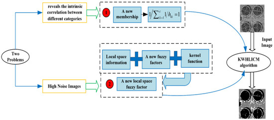
Figure 1.
The main framework of the proposed algorithm.
3.3.1. Robust Harmonic Fuzzy Clustering with Local Information
However, the above harmonic fuzzy C-means clustering algorithm has the same drawback as the classical FCM algorithm; i.e., it is very sensitive to noise and outliers. Inspired by the existing robust FLICM algorithm [21], this paper further proposes the harmonic fuzzy local information C-means (HLICM) algorithm to solve the above problem. The optimization model of the robust harmonic fuzzy algorithm for image segmentation is constructed as follows:
- s.t. (a) ; (b) ; (c) .
- where is the fuzzy weighting exponent and represents the harmonic fuzzy membership of each sample belonging to different categories.
Compared with the FLICM algorithm, the proposed algorithm replaces the Zadeh fuzzy set in the model with a harmonic fuzzy set, which establishes a harmonic fuzzy local information C-means clustering algorithm, and therefore, the above model is reasonable.
Using the Lagrange multiplier method, the unconstrained objective function is constructed as follows:
We find the partial derivatives of the objective function with respect to , , and and make them equal to zero.
- Solution
From Equation (34), it follows that
Substituting Equation (36) into Equation (35), we can obtain
In this way, we get
Substituting Equation (38) into Equation (36), we obtain
- 2.
- Solution
According to , we can obtain
To decrease the computational complexity, this clustering center is often approximated by the following equation:
Equations (41) and (39) are iterative formulas of the harmonic fuzzy membership and the clustering center, respectively, and they solve Equation (31) by alternately iterating between the harmonic fuzzy partition matrix and the clustering centers. The specific algorithmic algorithm 1 is described as follows:
| Algorithm 1 Harmonic fuzzy local information C-means clustering |
| Input Dataset X = {x1, x2,…, xn}, where is the number of samples. |
| Output and the clustering center matrix . |
| Initialization Set algorithm stopping error , set the maximum number of iterations of the algorithm , initialize the clustering center , set the number of iterations , and set the size of neighborhood window . |
| Repeat using Equation (39); using Equation (41); or the number of iterations of the algorithm , the algorithm ends; Otherwise, |
| End Algorithm is over. |
3.3.2. Harmonic Fuzzy Clustering with Weighted Local Information
However, due to the fact that the segmentation results and noise resistance of the HLICM algorithm are not as good as we expected, this paper was inspired by the KWFLICM algorithms [23], and a weighted local coefficient was introduced into the HLICM algorithm to construct a new robust fuzzy local clustering algorithm IHLICM with good noise immunity and segmentation performance. The optimization model of the IHLICM algorithm is constructed below:
- s.t. (a) ; (b) ; (c) .
- where is the fuzzy weighting exponent, which defaults to the range of [5, 10] and denotes the harmonic fuzzy membership of each sample belonging to different categories.
The weighted harmonic fuzzy local information factor is defined as follows:
Using the least squares method to solve this objective function, the updated formulas for harmonic fuzzy membership and the clustering center are obtained as follows:
To reduce the computational complexity, this clustering center is often approximated by the following formula:
3.3.3. Robust Kernelized Harmonic Fuzzy Clustering with Local Information
Two robust HCM algorithms have significant improvement in terms of noise resistance and segmentation performance, but there are still shortcomings compared to the KWFLICM algorithm. Therefore, this paper was once again inspired by the KWFLICM algorithm and proposes a novel high performance KWHLICM algorithm. The optimization model of the KWHLICM algorithm is constructed as follows:
- s.t. (a) ; (b) ; (c)
- where is the fuzzy weighting exponent, which defaults to the range of [5, 10], denotes the harmonic fuzzy membership of each sample belonging to different categories, and the kernel weighted harmonic fuzzy local information factor is defined as follows:
The weighted local coefficient in [23] consists of spatial information and neighborhood gray scale information . The least squares method is used to solve this objective function to obtain the updated formulas for harmonic membership and the clustering center, respectively, as follows:
To reduce the computational complexity, this clustering center is often approximated by the following formula:
Similar to the KWFLICM algorithm, the proposed KWHLICM algorithm also combines the neighborhood spatial information and grayscale features to establish a new fuzzy local information factor, which greatly improves the robustness of the algorithm to noise. The KWHLICM algorithm tests a noisy image, with the dynamic iteration process for image segmentation shown in Figure 2.
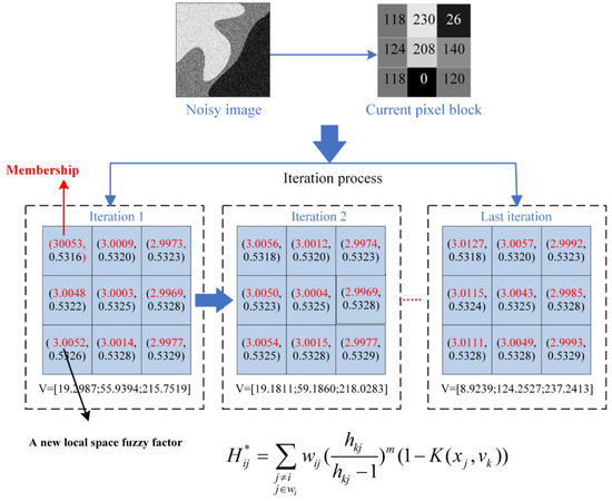
Figure 2.
Schematic diagram of dynamic iteration process for the proposed KWHLICM algorithm.
As shown in Figure 3, a 3 × 3 block of neighborhood pixels is selected from the noisy image. The iterative changes of fuzzy membership and the clustering centers intuitively reflect that the proposed algorithm is a two-level alternating iterative algorithm. In a neighborhood of the noisy image, we identify normal pixels with grayscale values of 118, 120, 124, and 140, and noisy pixels with grayscale values of 0, 26, 208, and 230. In the first iteration, the membership of the noise pixels is relatively low, and after several iterations using the KWHLICM algorithm, noisy pixels and surrounding pixels have similar membership. The iterated results show that the proposed KWHLICM algorithm can effectively suppress the effect of noise on this fuzzy clustering algorithm.
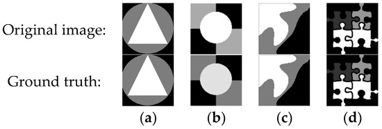
Figure 3.
Synthetic image. (a) Regular image with three classes; (b) regular image with three classes; (c) irregular image with three classes; and (d) regular image with three classes.
In summary, these two improved algorithms have a similar process to the HLICM algorithm; they are not repeated here due to the limited length of this paper.
3.4. Algorithm Convergence Analysis
Only the convergence of alternating iterative algorithms can ensure their effectiveness and rationality. So far, the related algorithms for fuzzy C-means clustering with constraints as additive expressions have been rigorously proved to be locally convergent and have been widely used in pattern analysis and data mining [50,51]. Saha and Das [52] provided a general convergence analysis method for iterative algorithms using Zangwill’s theorem. This paper uses this method to analyze the convergence of the proposed HLICM algorithm. If the objective function of the HLICM algorithm is decreasing, it indicates that the algorithm is convergent.
Considering the limited length of this paper, the proof of continuity and tightness constraints for the HLICM algorithm is the same as that for the FCM algorithm [53,54,55], and the IHLICM and KWHLICM algorithms are similar to the HLICM method. Therefore, in this article, we only prove that the objective function of the HLICM algorithm is a decreasing function, thus omitting the proof of the other two constraints in the theorem and the subsequent proof of the proposed algorithm.
Theorem 1.
[56] (Lagrange’s Theorem). Let functions , and , , , be continuously partially differentiable and let be a local extreme point of the function subject to the constraints , . and at the point . Then, we have that the gradient of at the point is 0, i.e., .
Theorem 2.
[56] (local sufficient conditions). Let functions , and , , , be continuously partially differentiable and let be a solution of the system . Let be the bordered Hessian matrix and consider its leading principle minors of the order at point . Therefore, the following expressions can be derived:
- (1)
- If all leading principle minors , , have the sign , then is a local minimum point of function subject to the constraints .
- (2)
- If the signs of all leading principle minors , , are alternated, the sign of being that of then is a local minimum point of functions subject to the constraints .
- (3)
- If neither the conditions of (1) nor those of (2) are satisfied, then is not a local extreme point of function subject to the constraints . Here, the case in which one or several leading principal minors have a value of zero is not considered a violation of conditions (1) or (2).
For the optimization model of the HLICM algorithm, using constraint , the final constructed unconstrained objective function is constructed as follows:
where .
If is a decreasing function, then the following three propositions should hold true
Proposition 1.
Given a clustering center , let , if and only if Equation (39) is computed to obtain , is a minima of function .
Proof.
Given , if it is assumed that the minimum point of is , then
Finally, we can obtain
Subsequently, we find the Hessian matrix of function when
As a result, we obtain
According to Equation (58), this Hessian matrix is positive definite when However, for the HLICM algorithm, it only makes sense when . Therefore, this Hessian matrix is positive definite when takes any real number greater than 0.
At the same time, we can know that the sufficient condition for determining the strict minima of the objective function is to analyze the Jacobi and Hessian matrices. Therefore, in addition to the above analysis, we also need to evaluate the bordered Hessian matrix [56]. Given the clustering center matrix , the bordered Hessian matrix of and is as follows:
For the leading principle minors of matrix are as follows:
According to the following bordered Hessian matrix theorem (local sufficient conditions), is the local minimum point in the condition of . □
Proposition 2.
Given , let if and only if Equation (40) is solved for . is a minima of the function .
Proof.
Given , if it is assumed that is a minima of the function , then
Finally, we obtain the Hessian matrix of function in
According to Equation (65), all diagonal elements of this Hessian matrix are greater than 0 and all off-diagonal elements are 0. Therefore, this Hessian matrix is positive definite. □
Through the previous deduction, this paper can conclude that the objective function of the HLICM algorithm decreases accordingly. In addition, the proof of the proposed algorithms with continuity and compactness constraints is similar to the proof of the FCM algorithm [54,55]. Overall, according to Zangwill’s theorem, the proposed HLICM algorithm is locally convergent. Since the IHLICM and KWHLICM algorithms are improved algorithms of HLICM and their derivation principles are similar to those of the HLICM algorithm, after proving that the HLICM algorithm is locally convergent, we can also show that the two improved algorithms proposed in this paper are also locally convergent, which can be proved in the same way as above.
4. Experimental Results and Analysis
To verify the effectiveness of the proposed algorithm, we selected grayscale images and color natural images for segmentation testing and compared the test results of the proposed algorithm to the following algorithms: ARFCM [57], FLICMLNLI [58], FCM-VMF [59], DSFCMN [60], KWFLICM [23], PFLSCM [61], FCM-SICM [62], FSC-LNML [63], and FLICM [21]. In addition, Gaussian noise, Rician noise, speckle noise, and salt and pepper noise were added to these images and the segmentation results of these noisy images were manually observed for evaluation. Therefore, we used many evaluation metrics, such as accuracy (Acc), sensitivity (Sen), the Jaccard coefficient, segmentation accuracy (SA), the Kappa coefficient (Kappa), mean intersection over union (mIoU), peak signal noise ratio (PSNR), and the Dice similarity coefficient (DICE) to objectively evaluate the segmentation results. During the testing process, the local neighborhood window size of the HLICM algorithm was 3 × 3, with a fuzzy weighting exponent of 2.0. The local neighborhood window size of the IHLICM and KWHLICM algorithms was 3 × 3, with a range of fuzzy weighting exponents of [5, 10]. A hardware platform with CPU-i7, 2.70 GHz, and 16.0 GB RAM was tested on the Matlab r2021b software platform in the Windows 11 environment. For the comparison algorithms, the local neighborhood window sizes of the ARFCM, FLICMLNLI, FCM_VMF, DSFCM_N, KWFLICM, PFLSCM, FCM_SICM, FSC_LNML, and FLICM algorithms were 5 × 5, 3 × 3, 4 × 4, 3 × 3, 3 × 3, 3 × 3, 7 × 7, 7 × 7, and 3 × 3, respectively. The number of clusters in fuzzy clustering algorithm for image segmentation is determined according to the Matlab-based clustering validity index toolbox [64]. For the convenience of description, this section uses to denote the mean value of Gaussian noise, represents the normalized variance of Gaussian noise, denotes the intensity level of salt and pepper noise, and denotes the standard deviation of Rician noise. For example, Gaussian noise with a mean value of 0 and normalized variance of 0.1 is represented as GN(0, 0.1), salt and pepper noise with an intensity of 30% is represented as SPN(0.3), speckle noise with a normalized variance of 0.2 is represented as SN(0.2), and Rician noise with a standard deviation of 80 is represented as RN(80).
4.1. Evaluation Indicators
4.1.1. Peak Signal-to-Noise Ratio (PSNR) [65]
Peak signal-to-noise ratio (PSNR) is an indicator used to measure the quality of an image or video. It is usually used to compare the difference between the original image and a compressed or processed image. PSNR is calculated using the following formula:
where represents the maximum possible value of image pixels and is the mean squared error (MSE), which represents the square of the average difference in pixel values between the original image and the processed image. The higher the PSNR value, the better the image quality, as this means that the difference between the original image and the processed image is smaller.
4.1.2. Segmentation Accuracy (SA) [57]
Image segmentation is the process of dividing an image into different regions or objects, and segmentation accuracy is the evaluation of the degree of similarity between the segmentation results and the ground truth.
4.1.3. Mean Intersection over Union (mIoU) [66]
The average intersection and merger ratio is an indicator used to evaluate the quality of image segmentation, which is the average of IoU (intersection and merger ratio). The mIoU index integrates the degree of similarity between the segmentation results and the ground truth across all categories and is a commonly used indicator for segmentation accuracy.
In image segmentation tasks, the higher the mIoU value, the closer the segmentation result is to the ground truth, which means that the algorithm has better segmentation performance in different categories.
4.1.4. Accuracy (Acc), Sensitivity (Sen), the Jaccard Coefficient, and the DICE [67]
TP denotes true positive, TN denotes true negative, FP denotes false positive, and FN denotes false negative. The accuracy value ranges from 0 to 1. The closer the value is to 1, the higher the accuracy of classification or segmentation.
Accuracy
Sensitivity
Jaccard coefficient
Dice similarity coefficient (DICE)
Accuracy is the ratio of the number of correctly classified or segmented samples to the total number of samples in a classification or segmentation task. Sensitivity is the proportion of true cases correctly identified as positive cases, also known as the true case rate. The Jaccard coefficient, also known as Intersection over Union (IoU), is used to evaluate the similarity between two sets. In segmentation tasks, the Jaccard coefficient index is often used to evaluate the degree of overlap between the segmentation results and the ground truth. The Dice similarity coefficient (DICE) is a commonly used indicator to evaluate the quality of image segmentation and is also widely used to assess the performance of medical image segmentation tasks.
4.1.5. The Kappa Coefficient [67]
The Kappa coefficient considers the consistency between the classification or segmentation results and the ground truth, avoiding the limitation of relying solely on superficial indicators such as accuracy to evaluate performance.
4.2. Test and Analysis of Algorithm Robustness
4.2.1. Synthetic Images
To verify the robustness of the proposed algorithm, four synthetic images shown in Figure 3 were selected and various types of noise were added to these synthetic images for testing the proposed algorithm and all the comparison algorithms.
RN(80) was added to Figure 3a, GN(0, 0.1) was added to Figure 3b, SPN(0.2) was added to Figure 3c, and SN(0.2) was added to Figure 3d. These images with noise were segmented using various fuzzy clustering algorithms. The segmentation results are shown in Figure 4. Table 1 gives the evaluation metrics corresponding to the various algorithms.
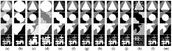
Figure 4.
Segmentation results of different algorithms for noisy synthetic images. (a) Noisy images; (b) ARFCM; (c) FLICMLNLI; (d) FCM_VMF; (e) DSFCM_N; (f) KWFLICM; (g) PFLSCM; (h) FCM_SICM; (i) FSC_LNML; (j) FLICM; (k) HLICM; (l) IHLICM; and (m) KWHLICM.

Table 1.
Evaluation indexes of different algorithms for the noisy synthetic images.
From Figure 4, it can be seen that when the image contains high noise, the segmentation results of the FCM_VMF and FLICM algorithms are poor, indicating that they do not have good noise resistance. The ARFCM algorithm has good noise resistance, but over-segmentation may occur. The PFLSCM and HLICM algorithms cannot effectively suppress the noise, while the FLICMLNLI algorithm can suppress the noise, but it can also cause over-segmentation of the image. The FCM_SICM and FSC_LNML algorithms can suppress noise, but their results have uneven edges. The DSFCM_N algorithm is robust to salt and pepper noise but sensitive to other types of noises. The KWFLICM and IHLICM algorithm can effectively suppress a large amount of noise, but the segmentation results are poor. The KWHLICM algorithm is more effective in synthetic images and is more suitable than the other comparison algorithms. From Table 1, it can be seen that the evaluation indexes of the KWHLICM algorithm are all higher than the other algorithms; therefore, the KWHLICM algorithm is universal best choice for segmenting images contaminated by noise.
4.2.2. Natural Images
To further test the performance of the algorithm, four natural images from BSDS500 [68] and VOC2010 [69] were selected for segmentation testing.
GN(0, 0.1) was added to Figure 5a,b and SPN(0.3) was added to Figure 5c,d. These images with noise were segmented using various fuzzy clustering algorithms. The segmentation results are shown in Figure 6. Table 2 gives the evaluation metrics corresponding to various algorithms.
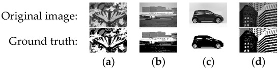
Figure 5.
Natural images. (a) 35010 from BSDS500; (b) 2007_000738 from VOC2010; (c) 2009_003974 from VOC2010; (d) 48017 from BSDS500.
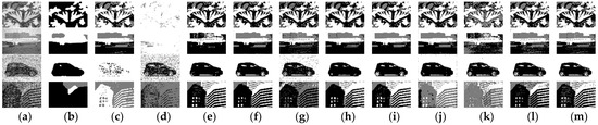
Figure 6.
Segmentation results of different algorithms for noisy natural images. (a) Noisy image; (b) ARFCM; (c) FLICMLNLI; (d) FCM_VMF; (e) DSFCM_N; (f) KWFLICM; (g) PFLSCM; (h) FCM_SICM; (i) FSC_LNML; (j) FLICM; (k) HLICM; (l) IHLICM; and (m) KWHLICM.
Table 2.
Evaluation indexes of different algorithms for natural images with noise.
From Figure 6, it can be seen that the ARFCM and KWFLICM algorithms can effectively suppress noise, but their segmentation results are not satisfactory. The FCM_VMF, DSFCM_N, and PFLSCM algorithms cannot effectively suppress noise. The FLICMLNLI algorithm can suppress most of the noise, but it is prone to over-segmentation. The FCM_SICM and FSC_LNML algorithms can still suppress noise, but they are prone to losing detailed information in the image during segmentation. The HLICM and FLICM algorithms can suppress some noise, but their segmentation results are also unsatisfactory. The KWHLICM algorithm can suppress a large amount of noise, indicating its robustness, and its segmentation results are the best among all the algorithms. Therefore, in summary, the KWHLICM algorithm has good application prospects for natural image segmentation.
4.2.3. Remote Sensing Images
To illustrate the effectiveness of the algorithm, four remote sensing images from the UC Merced Land Use dataset [70] were selected for segmentation testing.
SN(0.2) was added to Figure 7a,b, SPN(0.4) was added to Figure 7c,d, and these noisy images were segmented using various fuzzy clustering algorithms. The segmentation results are shown in Figure 8. Table 3 gives the evaluation metrics corresponding to the various algorithms.
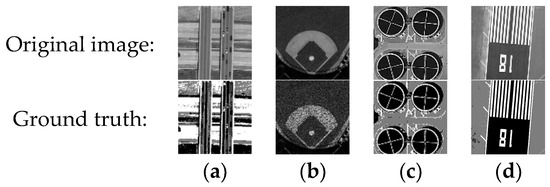
Figure 7.
Remote sensing images. (a) overpass91; (b) baseballdiamond03; (c) storagetanks42; and (d) runway22.
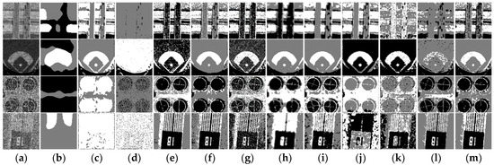
Figure 8.
Segmentation results of different algorithms for noisy remote sensing images. (a) Noisy image; (b) ARFCM; (c) FLICMLNLI; (d) FCM_VMF; (e) DSFCM_N; (f) KWFLICM; (g) PFLSCM; (h) FCM_SICM; (i) FSC_LNML; (j) FLICM; (k) HLICM; (l) IHLICM; and (m) KWHLICM.
Table 3.
Evaluation indexes of different algorithms for noisy remote sensing images.
From Figure 8, it can be seen that the ARFCM, KWFLICM, and FLICM algorithms can effectively suppress the noise, but their segmentation results are poor. The FCM_VMF, DSFCM_N, PFLSCM, and HLICM algorithms cannot effectively suppress the noise. The FLICMLNLI algorithm cannot effectively segment the image while suppressing the noise. The FCM_SICM and FSC_LNML algorithms can still suppress noise, but they are prone to losing detailed information in the image during segmentation. The KWHLICM algorithm can suppress a large amount of noise, indicating its robustness, and the segmentation results are the best among all the algorithms. In addition, from Table 3, for all the evaluation indexes, the proposed KWHLICM algorithm’s values are the highest among all the algorithms. In summary, the KWHLICM algorithm has good application prospects for remote sensing image segmentation.
4.2.4. Medical Images
To illustrate the effectiveness of the algorithm, four MR images were selected from the Brain Tumor MRI Dataset [71] for segmentation testing.
RN(80) was added to Figure 9a, RN(90) was added to Figure 9b, and GN(0, 0.1) was added to Figure 9c,d. These images with noise were segmented using various fuzzy clustering algorithms. The segmentation results are shown in Figure 10. Table 4 gives the evaluation metrics corresponding to the various algorithms.
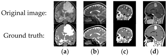
Figure 9.
MR images from Brain Tumor MRI dataset. (a) Tr-me_0180; (b) Te-no_0013; (c) 37 no; and (d) Tr-me_0235.
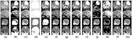
Figure 10.
Segmentation results of different algorithms for noisy MRI images. (a) Noisy image; (b) ARFCM; (c) FLICMLNLI; (d) FCM_VMF; (e) DSFCM_N; (f) KWFLICM; (g) PFLSCM; (h) FCM_SICM; (i) FSC_LNML; (j) FLICM; (k) HLICM; (l) IHLICM; and (m) KWHLICM.
Table 4.
Evaluation indexes of different algorithms for MR images with noise.
From Figure 10, it can see that the ARFCM, KWFLICM, FLICMLNLI algorithms can effectively suppress noise, but their segmentation results are not satisfactory. The FCM_VMF, PFLSCM, HLICM, and DSFCM_N algorithms cannot effectively suppress noise. The FCM_SICM and FSC_LNML algorithms can suppress noise, but often lose the detailed information of the image during the segmentation process. The KWFLICM algorithm can suppress noise while losing a lot of detail information, which is not what we want. The KWHLICM algorithm can suppress a large amount of noise, which indicates that it is robust and the segmentation result is the best among all algorithms. From Table 4, all the evaluation indexes of the proposed KWHLICM algorithm are the highest among all the algorithms. Therefore, in summary, the KWHLICM algorithm has good application prospects for MR image segmentation.
4.3. Testing and Analyzing the Effect of Noise Intensity on Algorithm Performance
Rician noise with a standard deviation of 50 to 80 was added to the medical image of Figure 9a. Noisy images were processed using 12 fuzzy clustering algorithms and the variation curves of the performance metrics of different algorithms with a standard deviation of Rician noise were obtained as shown in Figure 11. The variation of the evaluation metrics of most of the algorithms was not significant, and the FCM_VMF, HLICM and ARFCM algorithms have low evaluation metrics on medical images with Rician noise. With the increase of the standard deviation of the Rician noise, the evaluation metrics of the proposed KWHLICM algorithm have higher values than all the comparison algorithms, and therefore the KWHLICM algorithm is more stable and robust to changes in Rician noise.
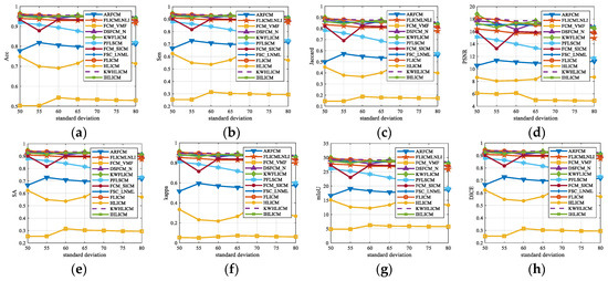
Figure 11.
Performance curves of different algorithms varying with standard deviation of Rician noise. (a) Acc; (b) Sen; (c) Jaccard; (d) PSNR; (e) SA; (f) Kappa; (g) mIoU; and (h) DICE.
Gaussian noise with different normalized variances was added to the synthetic images in Figure 3b. Segmentation tests were performed on these images using 12 algorithms and the variation curves of the evaluation metrics with the normalized variance of Gaussian noise were obtained, as shown in Figure 12. Most of the algorithms have insignificant variation of the evaluation metrics with noise, among which the HLICM, FCM_VMF, and ARFCM algorithms have lower evaluation metrics. Most of the performance metrics of the proposed KWHLICM method are better than all the comparison algorithms. In addition, the performance curve of the KWHLICM algorithm changes slowly with the normalized variance of Gaussian noise. Therefore, the proposed KWHLICM algorithm outperforms all the comparative algorithms in the presence of Gaussian noise.
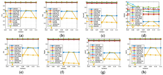
Figure 12.
Performance curves of different algorithms varying with the normalized variance of Gaussian noise. (a) Acc; (b) Sen; (c) Jaccard; (d) PSNR; (e) SA; (f) Kappa; (g) mIoU; and (h) DICE.
Salt and pepper noise with different intensity levels was added to the natural image in Figure 5c, 12 fuzzy clustering algorithms were used to segment these noisy images, and the curves of the evaluation metrics of the different algorithms varying with the strength of salt and pepper noise were obtained, as shown in Figure 13. Overall, the metrics of all the algorithms decrease with the increase of the intensity level of salt and pepper noise. When the noise intensity is less than 0.21, the metrics of the PFLSCM algorithm are higher than other algorithms, but with the increase of noise (when the noise intensity is stronger than 0.21), all the evaluation metrics of the KWHLICM algorithm are higher than other algorithms. In addition, the metrics of the ARFCM and FCM_VCM algorithms are very low. Therefore, the proposed KWHLICM algorithm outperforms all the comparison algorithms in the presence of salt and pepper noise.
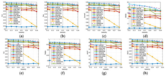
Figure 13.
Performance curves of different algorithms varying with the intensity of salt and pepper noise. (a) Acc; (b) Sen; (c) Jaccard; (d) PSNR; (e) SA; (f) Kappa; (g) mIoU; and (h) DICE.
Speckle noise with different normalized variances was added to the remote sensing image in Figure 9a, 12 fuzzy clustering algorithms were used to segment these noisy images, and the curves of the evaluation metrics of the different algorithms with the intensity of the speckle noise were obtained, as shown in Figure 14. As the normalized variance of the speckle noise increases, most of the evaluation metrics of all the algorithms decrease. The evaluation index value of the DSFCM_N algorithm is higher when the noise is lower than 0.05, but as the noise increases, the KWHLICM algorithm obtains higher evaluation values than all the comparison algorithms. The evaluation index values of the HLICM and FCM_VMF algorithms are generally low. Overall, the segmentation performance of the proposed KWHLICM algorithm is minimally affected by the variation of the noise, and it is more robust to speckle noise than all the comparison algorithms.
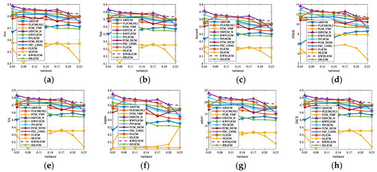
Figure 14.
Performance curves of different algorithms varying with standard deviation of Speckle noise. (a) Acc; (b) Sen; (c) Jaccard; (d) PSNR; (e) SA; (f) Kappa; (g) mIoU; and (h) DICE.
4.4. Analysis and Testing of Algorithm Complexity
Algorithm complexity is an important indicator for measuring algorithm performance. Table 5 gives the computational complexity of all the algorithms in this paper, where is the number of pixels in image, is the size of the local neighborhood window under robust fuzzy clustering, is the number of classes, is the number of iterations for algorithm convergence, is the size of the local neighborhood window under Gaussian and bootstrap bilateral filtering, is the size of the local neighborhood window under non-local mean filtering, and is the size of the local search window under non-mean filtering.
Table 5.
Computational complexity of different fuzzy clustering algorithms.
As shown in Table 5, the computational complexities of the ARFCM, FLICMLNLI, and PFLSCM algorithms are significantly higher than other compared algorithms. To verify the computational complexity of these algorithms, we tested and analyzed them using different images. By analyzing the time cost of these algorithms for processing noisy images, we confirmed the computational complexity of the algorithms covered in this paper. RN(80), GN(0, 0.1), SPN(0.3), and SN(0.2) were added to the two synthetic images in Figure 3b,d; SPN(0.3) and GN(0, 0.3) were added to the two natural images in Figure 5b,d; SPN(0.2) and SN(0.2) were added to the two remote sensing images in Figure 7a,c; and RN(80) and GN(0, 0.1) were added to two medical images in Figure 9a,d. Figure 15 shows the time cost bar chart of the different algorithms for these noisy images, where RN is Rician noise, SPN is salt and pepper noise, GN is Gaussian noise, and SN is speckle noise.
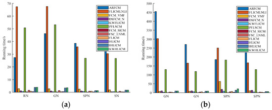
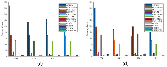
Figure 15.
Bar chart of time cost of different algorithms for noisy images. (a) Synthetic images; (b) natural images; (c) remote sensing images; (d) MR images.
As shown in Figure 15, the ARFCM, FLICMLNLI and PFLSCM algorithms consume significantly more time in processing noisy images than the other algorithms, and all three algorithms are relatively ineffective in segmenting images. However, the proposed KWHLICM, HLICM, and IHLICM algorithms consume less time but still struggle to meet the requirements of large-scale real-time image processing. In the near future, we will study fast algorithms related to the proposed algorithms [72,73] to meet the requirements of real-time image processing.
4.5. Impact of Neighborhood Size on Algorithm Performance
To investigate the influence of local neighborhood window size on the algorithm, we selected local domain windows of 3 × 3, 5 × 5, 7 × 7, 9 × 9, and 11 × 11 to test images with various types of noise and analyzed the segmentation results to determine the impact of local neighborhood window size on the algorithm.
GN(0, 0.1) was added to the synthetic image in Figure 3b, SPN(0.3) was added to the natural image in Figure 5d, SN(0.2) was added to the remote sensing image in Figure 7b, and RN(80) was added to the medical image in Figure 9a. The segmentation results of three proposed algorithms HLICM, IHLICM, and KWHLICM are shown in Figure 16, Figure 17 and Figure 18, respectively.
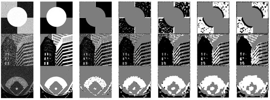
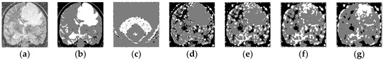
Figure 16.
Segmentation results of the proposed HLICM algorithm varying with the size of neighborhood window for noisy images. (a) Noisy image; (b) ground truths; (c) 3 × 3; (d) 5 × 5; (e) 7 × 7; (f) 9 × 9; and (g) 11 × 11.
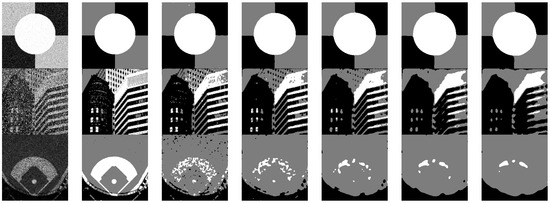
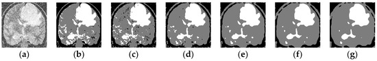
Figure 17.
Segmentation results of the proposed IHLICM algorithm varying with the size of neighborhood window for noisy images. (a) Noisy image; (b) ground truths; (c) 3 × 3; (d) 5 × 5; (e) 7 × 7; (f) 9 × 9; and (g) 11 × 11.

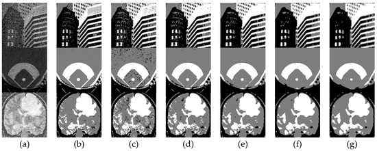
Figure 18.
Segmentation results of the proposed KWHLICM algorithm varying with the size of neighborhood window for noisy images. (a) Noisy image; (b) ground truths; (c) 3 × 3; (d) 5 × 5; (e) 7 × 7; (f) 9 × 9; and (g) 11 × 11.
4.5.1. Impact Testing of Neighborhood Window Size on HLICM
From Figure 16, it can be seen that although the tested image contains a small amount of noise, the segmentation results deteriorated as the neighborhood window size increased. From Table 6, it can be seen that when the neighborhood window size is 3 × 3, the segmentation evaluation index of the tested image was the highest. Therefore, the proposed HLICM algorithm can obtain satisfactory segmentation results when the neighborhood window size is 3 × 3.
Table 6.
Evaluation indexes of HLICM varying with neighborhood size for noisy images.
4.5.2. Impact Testing of Window Size on IHLICM
From Figure 17, although the tested image contains a small amount of noise, the segmentation results deteriorated as the window size increased. From Table 7, it can be seen that when the neighborhood window size is 3 × 3, the segmentation evaluation index of the tested image was the highest. Therefore, the proposed IHLICM algorithm can obtain satisfactory segmentation results when the neighborhood window size is 3 × 3.
Table 7.
Evaluation indexes of IHLICM varying with neighborhood size for noisy images.
4.5.3. Impact Testing of Window Size on KWHLICM
From Figure 18, it can be seen that when the neighborhood window size was 3 × 3, the segmentation results of the remote sensing images and medical images still contained a small amount of noise, which is not what we want, and when the neighborhood window size was 5 × 5, the noise was suppressed and the segmentation results were satisfactory. As the neighborhood window size continues to increase, the algorithm’s ability to suppress the noise is enhanced; however, some details are lost in image segmentation. From Table 8, it can be seen that when the neighborhood window size is 3 × 3, the segmentation evaluation index of the synthetic image is the highest, while when the neighborhood window size is 5 × 5, the segmentation evaluation index of the natural image, remote sensing image, and medical image is the highest. Therefore, it can be concluded that the KWHLICM algorithm can achieve satisfactory segmentation results when the window size is between 3 × 3 and 5 × 5.
Table 8.
Evaluation indexes of KWHLICM varying with window size for noisy images.
4.6. Impact of the Fuzzy Weighting Exponent on Algorithm Performance
The fuzzy weighting exponent is an important parameter in fuzzy clustering algorithms that has a certain impact on clustering performance. The range of the fuzzy weighting exponent varies depending on the algorithm. In general, the range of the fuzzy weighting exponent in FCM-related algorithms is between [1.5, 2.5] [74]. For the proposed harmonic fuzzy C-means clustering algorithm, we have conducted extensive experimental tests to confirm that its fuzzy weighting exponent is reasonably selected as [5,10]. Therefore, the HLICM, IHLICM, and KWHLICM algorithms proposed in this paper select values within this interval for testing and objectively analyze the impact of the fuzzy weighting exponent on its algorithm segmentation performance.
4.6.1. Fuzzy Weighting Exponent in HCM
This paper selected four representative numerical datasets (https://github.com/milaan9/Clustering-Datasets) (accessed on 15 October 2023) for clustering testing. These numerical data included Iris with 150 samples and four features, Triangle1 with 1000 samples and two features, Seeds with 210 samples and seven features, and Wine with 178 samples and thirteen features. The common accuracy (ACC) and normalized mutual information (NMI) indexes are used to evaluate the clustering performance of the proposed HCM algorithm, and the test results are displayed in Figure 19.
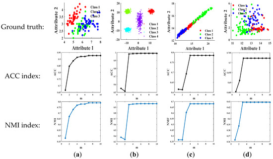
Figure 19.
Clustering evaluation results of the HCM algorithm varying with the fuzzy weighting exponent for numerical data. (a) Iris; (b) Triangle1; (c) Seeds; (d) Wine.
As shown in Figure 19, it can be seen that when , the ACC and NMI values basically do not change with the change of . Therefore, we conclude that the fuzzy weighting exponent in the HCM algorithm can be taken from 5.0.
In addition, we also selected four different types of images for segmentation testing. These images included an MRI brain image (https://www.kaggle.com/preetviradiya/brian-tumor-dataset) (accessed on 15 October 2023), two MSRC natural images (https://www.microsoft.com/en-us/research/project/image-understanding) (accessed on 15 October 2023), and an uneven illumination image. The common accuracy (ACC) and Jaccard similarity coefficient (Jaccard) were used to evaluate the segmentation performance of the proposed HCM algorithm, and the test results are displayed in Figure 20.
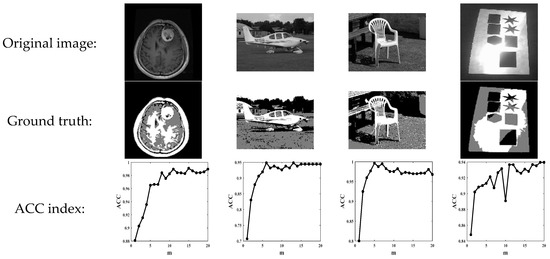
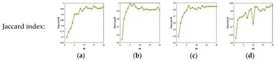
Figure 20.
Segmentation evaluation results of HCM algorithm varying with the fuzzy weighting exponent for image data. (a) Tr-me_0336; (b) 166_6645; (c) 112_1264; and (d) Uneven illumination image.
As shown in Figure 20, it can be seen that when the two indicators do not change much, and it can be concluded that for image data the reasonable range of the weighting exponent in the HCM algorithm should be greater than or equal to 5.
Based on the experimental results of Figure 19 and Figure 20, it can be seen that with the change of , the values of the ACC, NMI, and Jaccard change or unchanged within a small range, with basic fluctuations within 0.1. This indicates that the fuzzy weighting exponent in the HCM algorithm has almost no impact on the algorithm, so the reasonable range of the weighting exponent in the HCM algorithm for numerical data and image data is [5, 10].
Overall, it is precisely because the range of the fuzzy weighting exponent in the HCM algorithm is [5, 10] that we will also select the value range of the HLICM, IHLICM, and KWHLICM algorithms to be [5, 10].
4.6.2. The Fuzzy Weighting Exponent in the HLICM, IHLICM, and KWHLICM Algorithms
GN(0, 0.1) was used to corrupt the synthetic image in Figure 3b, SPN(0.3) was used to corrupt the natural image in Figure 5d, SN(0.2) was used to corrupt the remote sensing image in Figure 7b, and RN(80) was used to corrupt the MR image in Figure 9a. The proposed algorithm was tested with different fuzzy weighting exponents using corresponding noisy images. Figure 21 shows the curve of the algorithm performance as a function of the fuzzy weighting exponent.
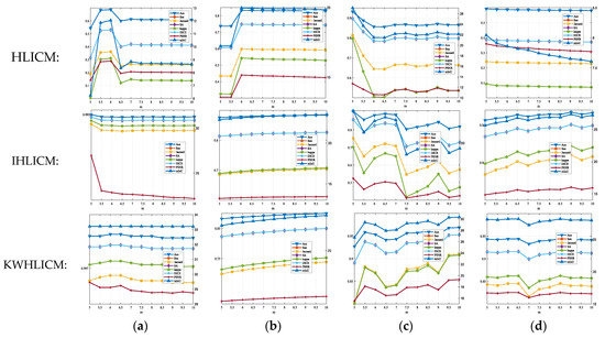
Figure 21.
Algorithm performance curve with various fuzzy weighting exponents. (a) Synthetic image with Gaussian noise; (b) natural image with salt and pepper noise; (c) remote sensing image with speckle noise; and (d) MR image with Rician noise.
As shown in Figure 21, the comparison of four types of noise shows that the three proposed algorithms are more sensitive to speckle noise, while for other three types of noise, these three algorithms are less sensitive to changes in the fuzzy weighting exponent. Overall, as the fuzzy weighting exponent changes, the performance of three proposed algorithms remains stable, and the range of fuzzy weighting exponents provided in the proposed algorithms is reasonable.
4.7. Impact of Initial Clustering Centers on Algorithm Performance
To verify the sensitivity of the algorithm to the initial clustering centers, the gray levels within the maximum and minimum values of the noisy image were equally divided into segments, and the gray levels with frequency 0 were removed. At each execution, a set of values from segment was selected as the initial clustering centers [75], and five sets of initial clustering centers were selected for segmentation testing. We selected the synthetic image in Figure 3b, which was polluted by Gaussian noise; the natural image in Figure 5d, which was corrupted by salt and pepper noise; the remote sensing image in Figure 7b, which was corrupted by speckle noise; and the MR image in Figure 9a, which was corrupted by Rician noise. Figure 22, Figure 23, Figure 24 and Figure 25 show a series of box plots of algorithm performance as a function of the initial clustering centers.
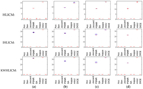
Figure 22.
Box plots of algorithm performance varying with initial clustering centers under Gaussian noise with different normalized variances. (a) GN(0, 0.05); (b) GN(0, 0.07); (c) GN(0, 0.1); and (d) GN(0, 0.12).
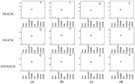
Figure 23.
Box plots of algorithm performance varying with initial clustering centers under salt and pepper noise with different intensity levels. (a) SPN(0.15); (b) SPN(0.2); (c) SPN(0.25); and (d) SPN(0.3).
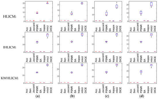
Figure 24.
Box plots of algorithm performance varying with different initial clustering centers under speckle noise with different normalized variances. (a) SN(0.05); (b) SN(0.1); (c) SN(0.15); and (d) SN(0.2).
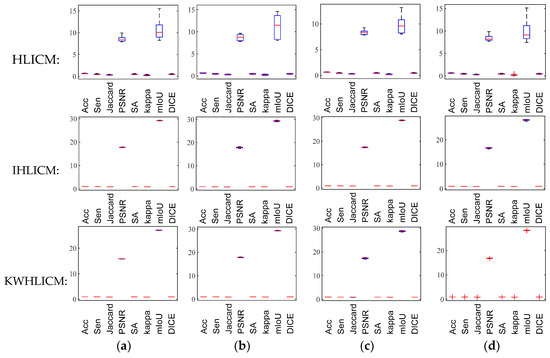
Figure 25.
Box plots of algorithm performance varying with different initial clustering centers under Rician noise with different standard deviations. (a) RN(50); (b) RN(60); (c) RN(70); and (d) RN(80).
As shown in Figure 22, Figure 23, Figure 24 and Figure 25, compared with images with different types of noise, the IHLICM and KWHLICM algorithms are more sensitive to the initial clustering centers on images containing speckle noise and salt and pepper noise, while the HLICM algorithm is more sensitive to the initial clustering centers on images containing Rician noise and speckle noise. These three proposed algorithms are insensitive to Gaussian noise, and overall, three proposed algorithms are not very sensitive to initial clustering centers.
4.8. Testing of the Algorithms’ Generalization Performance
To verify the adaptability of the algorithms, we select a large number of images from the BSDS500 dataset to verify the effectiveness and generalizability of the HLICM, IHLICM and KWHLICM algorithms. Considering the spatial limitation of this paper, only eight images from the BSDS500 dataset are provided and segmented using 12 fuzzy clustering algorithms. GN(0, 0.1) was used to corrupt #120003, #296028, #385028, and #353013 and SPN(0.3) was used to corrupt #56028, #140075, #223061, and #97033. The segmentation results of these algorithms for noisy natural images are shown in Figure 26.
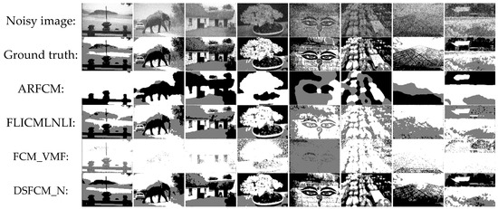
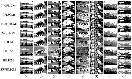
Figure 26.
Segmentation results of all algorithms for noisy images from the BSDS500 dataset. (a) 120003; (b) 296028; (c) 385028; (d) 353013; (e) 56028; (f) 140075; (g) 223061; and (h) 97033.
From Figure 26, it can be seen that the segmentation results of the FCM_VMF and FLICMLNLI algorithms are poor, indicating that these algorithms lack a certain robustness to noise. The FCM_VMF and FLICMLNLI algorithms have the worst segmentation effect on noisy images; the ARFCM algorithm loses a large amount of information in the image during segmentation; the segmentation results of the DSFCM_N, PFLSCM, FLICM, and HLICM algorithms contain a large amount of noise, which is unsatisfactory; the FCM_SCIM and FSC_LNML algorithms suppress a large amount of noise, but the edges of the segmented image are not smooth; and although the KWFLCM and IHLICM algorithms have a good performance in image segmentation, there is still noise in the segmentation results. Therefore, compared with other algorithms, the segmentation results of KWHLICM algorithm are closer to the ground truth and preserve many details. From Figure 27, it can be seen that KWHLICM outperforms other algorithms in terms of segmentation performance. Therefore, the KWHLICM algorithm has a significant advantage in segmenting natural images with noise.
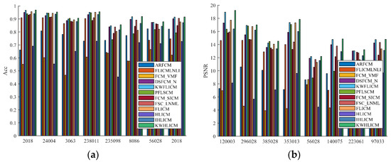
Figure 27.
Bar charts of Acc and PSNR indexes of different algorithms for noisy natural images. (a) ACC; (b) PSNR.
To further verify the generalizability of the algorithm, we continued by selecting a large number of images from the BSDS500 dataset for noise-free segmentation testing. The experimental results still show that KWHLICM still has good segmentation performance when segmenting noiseless images. Figure 28 show the segmentation results of eight noiseless natural images.
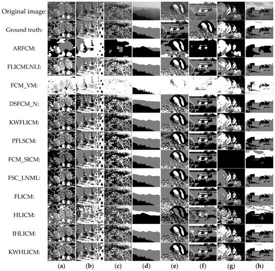
Figure 28.
Segmentation results of all algorithms for noise-free images from the BSDS500 dataset. (a) 208078; (b) 217090; (c) 8143; (d) 55067; (e) 106020; (f) 21077; (g) 306005; and (h) 197017.
From Figure 28, it can be seen that when segmenting natural images without noise, the ARFCM and FCM_VMF algorithms severely lose the detailed information of the image, while the FCM_SICM and FSC_LNML algorithms still blur the boundaries of the image when processing it. For #306005, the FCM_SICM algorithm failed to segment and for #106020 and #21077, the FSC_LNML algorithm cannot perform reasonable segmentation. Using the HLICM algorithm resulted in misclassification. For the FLICMLNLI, DSFCM_N, KWFLICM, PFLSCM, FLICM, KWHLICM and IHLICM algorithms, the difference in image segmentation results is small, and the naked eye cannot distinguish their differences well. From Figure 29, it can be seen that the ACC and PSNR values of the KWHLIMC algorithm are better than those of the other algorithms. Overall, the proposed KWHLICM algorithm for noise-free images has better generalization than existing fuzzy clustering-related algorithms.
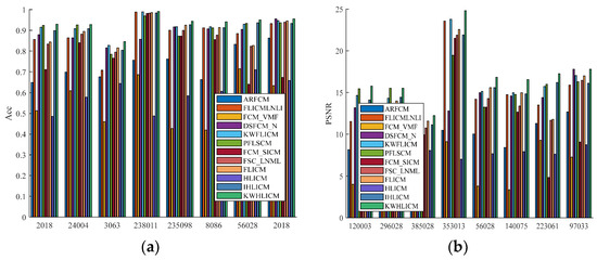
Figure 29.
Bar charts of Acc and PSNR indexes of different algorithms for noise-free natural images. (a) ACC; (b) PSNR.
4.9. Testing and Analysis of the Algorithms for Color Image
To verify the adaptability of the algorithm to color images, a large number of images from BSDS500 and UC Merced Land Use remote sensing datasets were selected to verify the generalizability and effectiveness of the proposed algorithm. SPN(0.2) was added to #296059# 304034, GN(0, 0.1) was added to #189011# 232038, and SN(0.2) was added to buildings18. Using 12 algorithms to segment these noise-free and noisy images, the segmentation results are shown in Figure 30.
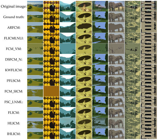
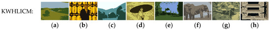
Figure 30.
Segmentation results of all algorithms for color images from the BSDS500 and UC Merced Land Use datasets. (a) 36046; (b) 65019; (c) 241004; (d) 189011; (e) 232038; (f) 296059; (g) 304034; and (h) buildings18.
From Figure 30, it can be seen that for noise-free color images, all algorithms except the ARFCM, FCM_VMF and FCM_SICM algorithms can effectively extract the target in the image. For color images contaminated by noise, the DSFCM-N, PFLSCM, FLICMLLI, FLICM and HLICM algorithms cannot completely suppress the noise, and the segmentation results still contain some noise. The ARFCM, FCMSCIM and FSC_LNML algorithms can suppress most of the noise in the image, but the edges of the segmented image are not smooth and satisfactory. The KWHLICM algorithm achieves better results, which are closer to the ground truths and also retain some details. From Figure 31, it can be seen that for both noiseless and noisy color images, the KWHLICM algorithm has higher metrics than other algorithms. Therefore, the proposed KWHLICM algorithm also has good universality for color image segmentation.
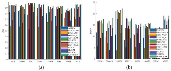
Figure 31.
Bar charts of ACC and PSNR indexes of different algorithms for color images with or without noise. (a) ACC; (b) PSNR.
4.10. Statistical Comparisons by the Friedman Test
To systematically compare different algorithms, this paper this paper uses the Friedman test [76] to evaluate the running efficiency (time) and segmentation quality (ACC, PSNR, and mIoU) of the 12 algorithms on the 16 images in Figure 3, Figure 5, Figure 7 and Figure 9. More specifically, the Friedman test rejects the null hypothesis that exhibits the same level of significance, which requires the use of the Nemenyi test for verification. If the average rankings of two algorithms differ by at least one key difference, their performance will be significantly different. The key difference is defined as . The CD plots are shown in Figure 32.
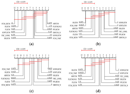
Figure 32.
CD diagrams of performance indexes of different algorithms for sixteen images. (a) Time; (b) ACC; (c) PSNR; and (d) mIoU.
According to the CD plots in Figure 32, the KWHLICM algorithm for 16 images has a statistical advantage over the other compared algorithms in terms of running efficiency and segmentation quality. In Figure 32a, the FLICMLNLI, PFLSCM, ARFCM, and DSFCM_N algorithms outperform the KWHLICM algorithm in terms of running efficiency. Therefore, the KWHLICM algorithm does not perform much better than these comparison algorithms in terms of runtime, but achieves a good compromise between segmentation quality and statistical running efficiency.
4.11. Algorithm Convergence Test
In this article, we monitor the convergence of the algorithm by calculating the number of iterations to determine if the change in the clustering centers that the algorithm converges to is below a preset threshold. Updating the cluster center is crucial during the clustering iteration process. When the change in the cluster center is less than the preset threshold, it can be considered that the iterative algorithm has converged and the cluster center has reached a stable state. To test the convergence of different algorithms, four images from the BSDS500, UC Merced land use, and brain tumor MRI datasets were selected for segmentation testing. Table 9 gives the algorithm iterations for different noisy images.
Table 9.
Iteration number of different algorithms for noisy images.
From Table 9, it can be seen that the HLICM algorithm has fewer iterations than the other algorithms, while the IHLICM and KHLICM algorithms have more iterations. However, by comparing the iteration times of different algorithms, it can be seen that the HLICM algorithm is significantly better than other compared algorithms in terms of convergence speed, while the convergence speed of the KWHLICM and IHLICM algorithms is not significantly different from other algorithms. Overall, the proposed KWHLICM and IHLICM algorithms not only have good segmentation performance, but also have high computational efficiency.
5. Conclusions and Outlook
This paper first defined the new concepts of harmonic fuzzy sets and harmonic fuzzy partition. Then, based on these basic concepts, a new harmonic fuzzy local information C-mean clustering algorithm was proposed, and the local convergence of this algorithm was rigorously proved using Zangwill’s theorem. Meanwhile, in order to improve the generalizability of the algorithms, as inspired by the IFLICM and KWFLCM algorithms, two enhanced robust image segmentation algorithms were proposed using local information, and their good performances were verified through experiments. In conclusion, the originality of our work lies in the integration of harmonic fuzzy membership and local spatial information in the clustering process:
- (1)
- The use of harmonic fuzzy partition to constrain fuzzy membership of all the algorithms;
- (2)
- In the proposed algorithm, sample clustering is performed by using harmonic fuzzy membership and neighborhood information of pixels;
- (3)
- The fuzzy membership degree in the proposed algorithm has a value range of , which is only supported by the harmonic fuzzy set theory proposed in this paper.
Overall, the proposed algorithms have satisfactory clustering results. These algorithms and related findings not only help to reveal the intrinsic structure of data, but also promote the development of fuzzy clustering related theories. Meanwhile, they can be widely used in data mining, image processing, and medical diagnosis. Clustering algorithms have important applications in various fields and can help people better understand data and make effective decisions.
There are many directions in which future work can be expanded. The following are some examples:
- (1)
- Explore the theory of harmonic fuzzy graphs [77] used to solve complex engineering problems;
- (2)
- Constructing harmonic fuzzy logic to solve problems related to fuzzy inference [78];
- (3)
- Construction of harmonic fuzzy neural networks [79,80] for solving complex engineering problems such as intelligent transportation and industrial automation.
Author Contributions
Conceptualization, C.W.; methodology, C.W. and S.Z.; writing—review and editing, C.W.; software, S.Z.; application to real data, S.Z.; and writing—original draft, S.Z. All authors have read and agreed to the published version of the manuscript.
Funding
This research received no external funding.
Data Availability Statement
All data used to support the findings of this study are included within the article.
Acknowledgments
The authors would like to thank everyone involved for their contributions to this article. They would also like to thank the anonymous reviewers for their helpful comments and suggestions.
Conflicts of Interest
The authors declare no conflicts of interest.
References
- Schaefer, A.; Scolaro, T.P.; Ghisi, E.E. Cluster analysis applied to obtaining reference models for building thermal performance studies. J. Build. Eng. 2024, 89, 109273. [Google Scholar] [CrossRef]
- Lee, M.; Hwang, S.; Park, Y.; Choi, B. Factors affecting bike-sharing system demand by inferred trip purpose: Integration of clustering of travel patterns and geospatial data analysis. Int. J. Sustain. Transp. 2022, 16, 847–860. [Google Scholar] [CrossRef]
- Yang, P.; Zhu, L.; Zhang, Y.; Ma, C.; Liu, L.; Yu, X.; Hu, W. On the relative value of clustering techniques for Unsupervised Effort-Aware Defect Prediction. Expert Syst. Appl. 2024, 245, 123041. [Google Scholar] [CrossRef]
- Taylor, H.H.; Bremner, A.J. Cluster kinds and the developmental origins of consciousness. Trends Cognit. Sci. 2024, 28, 586–587. [Google Scholar] [CrossRef]
- Yan, X.; Shi, K.; Ye, Y.; Yu, H. Deep correlation mining for multi-task image clustering. Expert Syst. Appl. 2022, 187, 115973. [Google Scholar] [CrossRef]
- Choi, S.; Lim, H.; Lim, J.; Yoon, S. Retrofit building energy performance evaluation using an energy signature-based symbolic hierarchical clustering method. Build. Environ. 2024, 251, 111206. [Google Scholar] [CrossRef]
- Gong, H.; Zhang, S.; Zhang, X.; Chen, Y. A method for chromatin domain partitioning based on hypergraph clustering. Comput. Struct. Biotec. 2024, 23, 1584–1593. [Google Scholar] [CrossRef]
- Mo, W.; Ni, S.; Zhou, M.; Wen, J.; Qi, D.; Huang, J.; Yang, Y.; Xu, Y.; Wang, X.; Zhao, Z. An electron density clustering based adaptive segmentation method for protein Raman spectrum calculation. Spectrochim. Acta A 2024, 314, 124155. [Google Scholar] [CrossRef] [PubMed]
- Laclau, C.; Nadif, M. Hard and fuzzy diagonal co-clustering for document-term partitioning. Neurocomputing 2016, 193, 133–147. [Google Scholar] [CrossRef]
- Zhi, X.; Fan, J.; Zhao, F. Robust local feature weighting hard c-means clustering algorithm. Neurocomputing 2014, 134, 20–29. [Google Scholar] [CrossRef]
- Ferreira, M.R.P.; Carvalho, F.A.T.; Simões, E.C. Kernel-based hard clustering methods with kernelization of the metric and automatic weighting of the variables. Pattern Recognit. 2016, 51, 310–321. [Google Scholar] [CrossRef]
- Dunn, J.C. A fuzzy relative of the ISODATA process and its use in detecting compact well separated clusters. J. Cybern. 1973, 3, 32–57. [Google Scholar] [CrossRef]
- Cardone, B.; Martino, F.D.; Senatore, S. Real estate price estimation through a fuzzy partition-driven genetic algorithm. Inf. Sci. 2024, 667, 120442. [Google Scholar] [CrossRef]
- Bezdek, J.C. Cluster validity with fuzzy sets. Cybernet. Syst. 1973, 3, 58–73. [Google Scholar] [CrossRef]
- Wu, J.; Wang, X.; Wei, T.; Fang, C. Full-parameter adaptive fuzzy clustering for noise image segmentation based on non-local and local spatial information. Comput. Vis. Image Underst. 2023, 235, 103765. [Google Scholar] [CrossRef]
- Mújica-Vargas, D.; Gallegos-Funes, F.; Rosales-Silva, A.J. A fuzzy clustering algorithm with spatial robust estimation constraint for noisy color image segmentation. Pattern Recogn. Lett. 2013, 34, 400–413. [Google Scholar] [CrossRef]
- Ahmed, M.N.; Yamany, S.M.; Mohamed, N.; Farag, A.A.; Moriarty, T. A modified fuzzy c-means algorithm for bias field estimation and segmentation of MRI data. IEEE Trans. Med. Imaging 2002, 21, 193–199. [Google Scholar] [CrossRef]
- Chen, S.; Zhang, D. Robust image segmentation using FCM with spatial constraints based on new kernel-induced distance measure. IEEE Trans. Syst. Man Cybern. Part B Cybern. 2004, 34, 1907–1916. [Google Scholar] [CrossRef]
- Szilagyi, L.; Benyo, Z.; Szilagyi, S.M.; Adam, H.S. MR brain image segmentation using an enhanced fuzzy C-means algorithm. In Proceedings of the Annual International Conference of the IEEE Engineering in Medicine and Biology Society(EMBC), Cancun, Mexico, 17–21 September 2003; pp. 17–21. [Google Scholar]
- Cai, W.; Chen, S.; Zhang, D. Fast and robust fuzzy c-means clustering algorithms incorporating local information for image segmentation. Pattern Recogn. 2007, 40, 825–838. [Google Scholar] [CrossRef]
- Krinidis, S.; Chatzis, V. A robust fuzzy local information C-means clustering algorithm. IEEE Trans. Image Process. 2010, 19, 1328–1337. [Google Scholar] [CrossRef]
- Li, Z.; Zheng, Z. Fuzzy C-mean clustering based on improved local information for MR image segmentation. Autom. Appl. 2024, 65, 225–228. [Google Scholar]
- Gong, M.; Liang, Y.; Shi, J.; Ma, W.; Ma, J. Fuzzy C-means clustering with local information and kernel metric for image segmentation. IEEE Trans. Image Process. 2013, 22, 573–584. [Google Scholar] [CrossRef] [PubMed]
- Leszczyński, K.; Penczek, P.; Grochulski, W. Sugeno’s fuzzy measure and fuzzy clustering. Fuzzy Sets Syst. 1985, 15, 147–158. [Google Scholar] [CrossRef]
- Li, J.J.; Zhang, L.; Yao, T.S. Convergence analysis of the GLCA algorithm. J. Comp. Res. Dev. 1999, 36, 978–981. [Google Scholar]
- Leski, J.M. Generalized weighted conditional fuzzy clustering. IEEE Trans. Fuzzy Syst. 2003, 11, 709–715. [Google Scholar] [CrossRef]
- Zadeh, L.A. Similarity relations and fuzzy ordering. Inf. Sci. 1971, 3, 177–200. [Google Scholar] [CrossRef]
- Huang, W.; Zhang, F.; Wang, S.; Kong, F. A novel knowledge-based similarity measure on intuitionistic fuzzy sets and its applications in pattern recognition. Expert Syst. Appl. 2024, 249, 123835. [Google Scholar] [CrossRef]
- Ruspini, E.H. A new approach to clustering. Inf. Control. 1969, 15, 22–32. [Google Scholar] [CrossRef]
- Ruspini, E.H. New experimental results in fuzzy clustering. Inf. Sci. 1973, 6, 273–284. [Google Scholar] [CrossRef]
- Pan, X.; Xu, Y. Redefinition of the concept of fuzzy set based on vague partition from the perspective of axiomatization. Soft Comput. 2018, 22, 1777–1789. [Google Scholar] [CrossRef]
- Mesiar, R.; Rybátrik, J. Entropy of fuzzy partitions: A general model. Fuzzy Sets Syst. 1998, 99, 73–79. [Google Scholar] [CrossRef]
- Torra1, V.; JurÍo, A.; Bustince, H.; Aliahmadipour, L. Fuzzy sets in clustering: On fuzzy partitions. Advances in Intelligent Systems and Computing. In Proceedings of the International Conference on Intelligent and Fuzzy Systems, INFUS 2019, Istanbul, Turkey, 23–25 July 2019; Springer: Cham, Switzerland, 2019; Volume 1029, pp. 7–14. [Google Scholar]
- Bezdek, J.C.; Harris, J.D. Fuzzy partitions and relations; an axiomatic basis for clustering. Fuzzy Sets Syst. 1978, 1, 111–127. [Google Scholar] [CrossRef]
- Torra, I.; Miyamoto, S. A definition for I-fuzzy partitions. Soft Comput. 2011, 15, 363–369. [Google Scholar] [CrossRef]
- Wang, J.; Chung, F.; Wang, S.; Deng, Z. Double indices-induced FCM clustering and its integration with fuzzy subspace clustering. Pattern Analysis Appl. 2014, 17, 549–566. [Google Scholar] [CrossRef]
- Zhu, J.; Li, K.; Xia, K.; Gu, X.; Xue, J.; Qiu, S.; Jiang, Y.; Qian, P. A novel double-index-constrained, multi-view, fuzzy-clustering algorithm and its application for detecting epilepsy electroencephalogram signals. IEEE Access 2019, 7, 103823–103832. [Google Scholar] [CrossRef]
- Zhang, X.; Juan, A.; Tauler, R. Local rank-based spatial information for improvement of remote sensing hyperspectral imaging resolution. Talanta 2016, 146, 1–9. [Google Scholar] [CrossRef]
- Siriapisith, T.; Kusakunniran, W.; Haddawy, P. Pyramid graph cut: Integrating intensity and gradient information for grayscale medical image segmentation. Comput. Biol. Med. 2020, 126, 103997. [Google Scholar] [CrossRef]
- Wu, C.; Zhang, X. A novel kernelized total Bregman divergence-based fuzzy clustering with local information for image segmentation. Int. J. Approx. Reason 2021, 136, 281–305. [Google Scholar] [CrossRef]
- Memon, K.H.; Lee, D.H. Generalised kernel weighted fuzzy C-means clustering algorithm with local information. Fuzzy Sets Syst. 2018, 340, 91–108. [Google Scholar] [CrossRef]
- Nik-Khorasani, A.; Mehrizi, A.; Sadoghi-Yazd, H. Robust hybrid learning approach for adaptive neuro-fuzzy inference systems. Fuzzy Sets Syst. 2024, 481, 108890. [Google Scholar] [CrossRef]
- Zadeh, L.A. Fuzzy sets. Inf. Control 1965, 8, 338–353. [Google Scholar] [CrossRef]
- Aggarwal, M. Redefining fuzzy entropy with a general framework. Expert Syst. Appl. 2021, 164, 113671. [Google Scholar] [CrossRef]
- Marín, N.; Rivas-Gervilla, G.; Sánchez, D.; Yager, R.R. Specificity measures based on fuzzy set similarity. Fuzzy Sets Syst. 2020, 401, 189–199. [Google Scholar] [CrossRef]
- Li, J.; Deng, G.; Li, H.; Zeng, W. The relationship between similarity measure and entropy of intuitionistic fuzzy sets. Inf. Sci. 2012, 188, 314–321. [Google Scholar] [CrossRef]
- Nagoev, Z.; Pshenokova, I.; Bzhikhatlov, K.; Kankulov, S.; Atalikov, B. Multi-agent neurocognitive architecture of an intelligent agent pattern recognition system. Procedia Comput. Sci. 2022, 213, 504–509. [Google Scholar] [CrossRef]
- Wu, C.; Li, M. Generalized multiplicative fuzzy possibilistic product partition C-means clustering. Inf. Sci. 2024, 670, 120588. [Google Scholar] [CrossRef]
- Xu, Z. Priority weight intervals derived from intuitionistic multiplicative preference. IEEE Trans. Fuzzy Syst. 2013, 21, 642–654. [Google Scholar]
- Chen, J.; Zhu, J.; Jiang, H.; Yang, H.; Nie, F. Sparsity fuzzy C-means clustering with principal component analysis embedding. IEEE Trans. Fuzzy Syst. 2023, 31, 2099–2111. [Google Scholar] [CrossRef]
- Li, H.; Wei, M. Fuzzy clustering based on feature weights for multivariate time series. Knowl. Based Syst. 2020, 197, 105907. [Google Scholar] [CrossRef]
- Saha, A.; Das, S. Stronger convergence results for the center-based fuzzy clustering with convex divergence measure. IEEE Trans. Cybern. 2019, 49, 4229–4242. [Google Scholar] [CrossRef]
- Bezdek, J.C. A convergence theorem for the fuzzy ISODATA clustering algorithms. IEEE Trans. on Pattern Anal. Mach. Intell. 1980, 2, 1–8. [Google Scholar] [CrossRef] [PubMed]
- Yang, M.S. Convergence properties of the generalized fuzzy C-means clustering algorithms. Comput. Math. Appl. 1993, 25, 3–11. [Google Scholar] [CrossRef]
- Gröll, L.; Jäkel, J. A new convergence proof of fuzzy C-means. IEEE Trans. Fuzzy Syst. 2005, 13, 717–720. [Google Scholar] [CrossRef]
- Tian, Y.; Yang, M.S. Bias-correction fuzzy clustering algorithms. Inf. Sci. 2015, 309, 138–162. [Google Scholar]
- Gao, Y.; Wang, Z.; Xie, J.; Pan, J. A new robust fuzzy c-means clustering method based on adaptive elastic distance. Knowl. Based Syst. 2022, 237, 107769. [Google Scholar] [CrossRef]
- Zhang, X.; Sun, Y.; Liu, H.; Hou, Z.; Zhao, F.; Zhang, C. Improved clustering algorithms for image segmentation based on non-local information and back projection. Inf. Sci. 2021, 550, 129–144. [Google Scholar] [CrossRef]
- Zhang, H.; Li, H.; Chen, N.; Chen, S.; Liu, J. Novel fuzzy clustering algorithm with variable multi-pixel fitting spatial information for image segmentation. Pattern Recogn. 2022, 121, 108201. [Google Scholar] [CrossRef]
- Ghosh, S.; Hazarika, A.P.; Chandra, A.; Mudi, R.K. Adaptive neighbor constrained deviation sparse variant fuzzy C-means clustering for brain MRI of AD subject. Visual Inf. 2021, 5, 67–80. [Google Scholar] [CrossRef]
- Tang, Y.; Ren, F.; Pedrycz, W. Fuzzy C-Means clustering through SSIM and patch for image segmentation. Appl. Soft Comput. 2020, 87, 105928. [Google Scholar] [CrossRef]
- Wang, Q.; Wang, X.; Fang, C.; Yang, W. Robust fuzzy c-means clustering algorithm with adaptive spatial & intensity constraint and membership linking for noise image segmentation. Appl. Soft Comput. 2020, 92, 106318. [Google Scholar]
- Wei, T.; Wang, X.; Li, X.; Zhu, S. Fuzzy subspace clustering noisy image segmentation algorithm with adaptive local variance non-local information and mean membership linking. Eng. Appl. Artifi. Intell. 2022, 110, 104672. [Google Scholar] [CrossRef]
- José-García, A.; Gómez-Flores, W. CVIK: A Matlab-based cluster validity index toolbox for automatic data clustering. SoftwareX 2023, 22, 101359. [Google Scholar] [CrossRef]
- Wang, Q.; Wang, X.; Fang, C.; Jiao, J. Fuzzy image clustering incorporating local and region-level information with median memberships. Appl. Soft Comput. 2021, 105, 107245. [Google Scholar] [CrossRef]
- Gharieb, R.R.; Gendy, G.; Selim, H. A hard C-means clustering algorithm incorporating membership KL divergence and local data information for noisy image segmentation. Int. J. Pattern Recogn. 2018, 32, 1850012. [Google Scholar] [CrossRef]
- Zheng, X.; Chen, T. High spatial resolution remote sensing image segmentation based on the multiclassification model and the binary classification model. Neural Comput. Appl. 2023, 35, 3597–3604. [Google Scholar] [CrossRef]
- Available online: https://www2.eecs.berkeley.edu/Research/Projects/CS/vision/grouping/resources.html (accessed on 10 March 2024.).
- Visual Object Classes Challenge 2012 (VOC2012). Available online: http://host.robots.ox.ac.uk/pascal/VOC/voc2012/index.html (accessed on 12 March 2024).
- UC Merced Land Use Dataset. Available online: http://weegee.vision.ucmerced.edu/datasets/landuse.html (accessed on 14 March 2024).
- Brain Tumor MRI Dataset. Available online: https://www.kaggle.com/datasets/masoudnickparvar/brain-tumor-mri-dataset (accessed on 16 March 2024).
- Hu, L.; Pan, X.; Tan, Z.; Luo, X. A fast fuzzy clustering algorithm for complex networks via a generalized momentum method. IEEE Trans. Fuzzy Syst. 2022, 30, 3473–3485. [Google Scholar] [CrossRef]
- Zhang, X.; Dai, L. Fast bilateral filtering. Electron. Lett. 2019, 55, 258–260. [Google Scholar] [CrossRef]
- Pal, N.R.; Bezdek, J.C. On clustering validity for the fuzzy C-means model. IEEE Trans. Fuzzy Syst. 1955, 3, 370–379. [Google Scholar] [CrossRef]
- Wu, C.; Guo, X. A novel single fuzzifier interval type-2 fuzzy C-means clustering with local information for land-cover segmentation. IEEE J. Sel. Top. Appl. Earth Obs. Remote Sens. 2021, 14, 5903–5917. [Google Scholar] [CrossRef]
- Demšar, J. Statistical comparisons of classifiers over multiple data sets. J. Mach. Learn. Res. 2006, 7, 1–30. [Google Scholar]
- Bhattacharya, A.; Pal, M. A fuzzy graph theory approach to the facility location problem: A case study in the Indian banking system. Mathematics 2023, 11, 2992. [Google Scholar] [CrossRef]
- Pal, M.; Jana, C.; Bhattacharya, A. Fundamentals of Fuzzy Optimization and Decision-Making Problems; Springer: Cham, Switzerland, 2023; pp. 1–30. [Google Scholar]
- Bhattacharya, A.; Pal, M. Prediction on nature of cancer by fuzzy graphoidal covering number using artificial neural network. Artif. Intell. Med. 2024, 148, 102783. [Google Scholar] [CrossRef] [PubMed]
- Li, K.; Ni, T.; Xue, J.; Jiang, Y. Deep soft clustering: Simultaneous deep embedding and soft-partition clustering. J. Amb. Intell. Hum. Comp. 2023, 14, 5581–5593. [Google Scholar] [CrossRef]
Disclaimer/Publisher’s Note: The statements, opinions and data contained in all publications are solely those of the individual author(s) and contributor(s) and not of MDPI and/or the editor(s). MDPI and/or the editor(s) disclaim responsibility for any injury to people or property resulting from any ideas, methods, instructions or products referred to in the content. |
© 2024 by the authors. Licensee MDPI, Basel, Switzerland. This article is an open access article distributed under the terms and conditions of the Creative Commons Attribution (CC BY) license (https://creativecommons.org/licenses/by/4.0/).