Modeling Pollutant Diffusion in the Ground Using Conformable Fractional Derivative in Spherical Coordinates with Complete Symmetry

Abstract

The conformal fractional derivative (CFD) has become a hot research topic since it has a physical interpretation and is easier to grasp and apply to problems compared with other fractional derivatives. Its application to heat transfer, diffusion, diffusion-advection, and wave propagation problems can be found in the literature. Fractional diffusion equations have received great attention recently due to their applicability in physical, chemical, and biological processes and engineering. The diffusion of the pollutants within the ground, which is an important environmental problem, can be modeled with a diffusion equation. Diffusion in some porous materials or soil can be modeled more accurately with fractional derivatives or the conformal fractional derivative. In this study, the diffusion problem of a spilled pollutant leaking into the ground modeled with the conformal fractional time derivative in spherical coordinates has been solved analytically using the Fourier series for a constant mass flow rate and complete symmetry under the assumptions of homogeneous and isotropic soil, constant soil temperature, and constant permeability. The solutions have been simulated spatially and in time. A parametric analysis of the problem has been performed for several values of the CFD order. The simulation results are interpreted. It has also been suggested how to find the parameters of the soil to see whether the CFD can be used to model the soil or not. The approach described here can also be used for modeling pollution problems involving different boundary conditions.

1. Introduction

The concept of fractional derivatives (FDs) dates back to a personal communication between Leibniz and l’Hôpital in the late 17th century [1]. Since then, numerous mathematicians, including Euler, Lagrange, Abel, and Liouville, have made significant contributions to the field. Unlike classical derivatives, fractional derivatives do not have a single definition, leading to various interpretations and transitions between definitions [1,2].

Common definitions in the literature include the Caputo, Riemann–Liouville, and Grunwald–Letnikov FDs [1,3,4]. For instance, while the Caputo FD of a constant is zero, the Riemann–Liouville FD yields a non-zero result when the lower bound is finite [1]. Originally confined to abstract mathematics, fractional-order derivatives (FODs), fractional integrals (FIs), and fractional differential equations (FDEs) have gained popularity over recent decades, largely due to advances in computer technology [2,5]. These concepts are now applied across various fields of applied sciences, including fluid mechanics, heat transfer, and diffusion [5,6], enhancing modeling accuracy in applied mathematics, engineering, physics, finance, chemistry, biology, bioengineering, electromagnetics, and hydrology [5,6,7,8].

The diffusion equation (DE) is crucial for describing the diffusion of particles, fields, or energy and is widely used in chemistry, physics, and mathematics [9,10]. In recent years, modeling diffusion processes using fractional-order derivatives, leading to fractional diffusion equations (FDEs), has become increasingly prevalent [6,7,8]. Langlands and Henry [10] examined the stability and accuracy of an easy-to-implement implicit numerical method according to finite difference approaches required for solving an FDE. They provided algebraic and numerical proofs for the range of the fractional order in which the method has unconditional stability for 0 < α < 1. By taking 0 < α < 2 in the classical DE, the FDE is obtained. In the case of 1 < α < 2, the equation is called the fractional diffusion wave or super-diffusion equation, and in the case of 0 < α < 1, it is called the sub-diffusion equation [6]. Furthermore, numerical methods have been extensively employed to solve FDEs, with various studies exploring stability, accuracy, and specific techniques such as the finite difference method, Crank–Nicolson discretization, and homotopic perturbation methods [6,9,10,11,12,13,14,15].

A compact finite difference scheme (CFDS) was developed for a time-fractional convection-diffusion equation (TF-CDE) to address the issue of groundwater pollution [16]. Additionally, a generalization of the classical advection-diffusion equation (ADE) was proposed, where the first-order space derivative is replaced by a Caputo or Riemann–Liouville derivative of 0 < β ≤ 1, and the second-order space derivative is substituted with a Caputo or Riemann–Liouville fractional derivative of order 1 < α ≤ 2. The solution to this new equation was derived using the Laplace transform, resulting in expressions involving Mittag-Leffler functions [17].

Despite the advancements, existing fractional derivatives often do not meet the original criteria [2,3]. Khalil et al. [18] introduced a conformable fractional derivative (CFD) that aligns more closely with the ordinary derivative, providing more intuitive product and quotient rules [19,20,21]. The CFD is more physically interpretable [21] and easier to apply in solving fractional-order differential equations [22,23,24] and finding applications in wave propagation, heat transfer, and diffusion in porous media [25,26,27,28,29,30]. Due to population increase, farming, and industrial activities worldwide, the release of large amounts of organic and inorganic compounds has become a major environmental problem [31]. Pollutants transferred by streams to their surroundings through diffusion cause soil and water pollution. Protecting surface and underground water resources is crucial, given their dwindling numbers. Moreover, the accumulation of pollutants in the soil affects soil fertility and the health of animals and humans as they pass through the food chain [32]. The diffusion equation (DE) is essential for describing the diffusion of various physical quantities such as particles, fields, or energy. Solutions to DEs of different types can reveal how deeply a pollutant infiltrates a medium [33,34,35,36]. The traditional DE is a parabolic equation widely used in chemistry, physics, mathematics, and many applied fields [9,10]. However, in recent decades, the use of fractional-order derivatives to model the diffusion process with non-integer order diffusion equations, or fractional diffusion equations (FDEs), has gained popularity [37,38,39,40,41,42,43]. Recent applications of the conformable fractional derivative in pollutant diffusion problems highlight its utility [44,45]. The Caputo fractional derivative has also been employed to model chloride diffusion in concrete, demonstrating superior performance compared to integer-order diffusion equations [46]. For example, Mirza et al. [47] used the conformable fractional derivative to derive a fractional-order diffusion equation and solved it analytically using the separation of the variables method.

The increasing prevalence of soil contamination from industrial and agricultural discharges, along with improper solid waste disposal, underscores the importance of developing accurate models to understand contaminant behavior in soil environments. Diffusion problems have been modeled using both ordinary and fractional-order derivatives, as evidenced in the literature. However, analytical solutions to diffusion phenomena in porous soils, particularly those considering different boundary conditions and dimensions, are still lacking. The CFD usage is relatively new in the literature, and its solution gives similar results to that obtained by the other FODs [18,19,24]. There are only a few papers about the CFD usage in modeling of diffusion phenomenon [30,44,45,46,47]. To the best of our knowledge, a CFD-based diffusion equation has not yet been used in three dimensions in the literature. Such a diffusion model can give simpler analytical solutions than the well-known FDs such as Caputo, Riemann–Liouville, and Grunwald–Letnikov. Without needing any numerical solutions, FDs can be used to examine the diffusion problem rapidly by taking different boundary conditions into account easily. Therefore, this study aims to address this gap by solving the diffusion problem in the soil where the time derivative of the diffusion equation is replaced with a conformable fractional time derivative. The model will focus on a point pollutant source in spherical coordinates, assuming a constant mass flow rate and complete spherical symmetry. The solution will be derived using the separation of the variables technique and Fourier series, providing insights into the impact of diffusion from a pollutant source of negligible physical dimensions.

2. Materials and Methods

2.1. Diffusion Equation in Spherical Coordinates with Conformal Fractional Time-Derivative

The CFD, developed in the last decade, has become a popular modeling and analysis method, and it is easier to use and comprehend than other FDs [18,20,21]. According to Khalil et al. [18], the CFD is defined as follows:

$${\displaystyle \frac{d^{\alpha }f\left(t\right)}{d{t}^{\alpha }}}=f^{\prime }\left(t\right)t^{1-\alpha }=C_{\alpha }{\displaystyle \frac{df\left(t\right)}{dt}}{t}^{1-\alpha }$$

(1)

where $0<\alpha \le 1$.

The DE in spherical coordinates is expressed in Equation (2):

$${\displaystyle \frac{\partial u}{\partial t}}=D\Delta u=\mathrm{D}\left({\displaystyle \frac{1}{r^2}}{\displaystyle \frac{\partial }{\partial r}}\left(r^2{\displaystyle \frac{\partial u}{\partial r}}\right)+{\displaystyle \frac{1}{r^2{\sin }^2\varphi }}{\displaystyle \frac{{\partial }^{2}u}{\partial {\theta }^2}}+{\displaystyle \frac{1}{r^2{\sin }^2\varphi }}{\displaystyle \frac{\partial }{\partial \varphi }}\left(\sin \varphi {\displaystyle \frac{\partial u}{\partial \varphi }}\right)\right)$$

(2)

where $u\left(r,\theta ,\varphi , t\right)$ represents the contaminant concentration in the soil; r is the distance from the source; θ is the zenith angle; ϕ is the azimuth angle; t is the time; and D (m²/s) is the diffusion coefficient of the contaminant in the soil. The DE in some soils is modified to have an FOD to match the experimental results [47]. By replacing the time derivative of Equation (2) with a fractional time derivative as performed in [48], the following fractional order differential equation in spherical coordinates can be obtained:

$${\displaystyle \frac{{\partial }^{\alpha }u\left(r,t\right)}{\partial t^{\alpha }}}=D_{\alpha }\Delta u=D_{\alpha }\left({\displaystyle \frac{1}{r^2}}{\displaystyle \frac{\partial }{\partial r}}\left(r^2{\displaystyle \frac{\partial u}{\partial r}}\right)+{\displaystyle \frac{1}{r^2{\sin }^2\varphi }}{\displaystyle \frac{{\partial }^{2}u}{\partial {\theta }^2}}+{\displaystyle \frac{1}{r^2{\sin }^2\varphi }}{\displaystyle \frac{\partial }{\partial \varphi }}\left(\sin \varphi {\displaystyle \frac{\partial u}{\partial \varphi }}\right)\right)$$

(3)

where $D_{\alpha }$ is the generalized diffusion coefficient (m²/s^α). The Caputo fractional derivative has been used in [48] and, therein, it has been shown that the use of FOD predicts the groundwater flow better in cylindrical coordinates based on experimental data. Diluted pollutants may obey a similar diffusion differential equation to the one in [48]. The CFD will be considered instead of the other fractional derivatives due to its simplicity, explicitness, and easiness in this study to find an analytical solution that is easier than the one given in [48]. If the CFD replaces the FOD in Equation (3), the following diffusion equation is obtained:

$${\displaystyle \frac{\partial u}{\partial t}}{t}^{1-\alpha }=D_{\alpha }\Delta u=D_{\alpha }\left({\displaystyle \frac{1}{r^2}}{\displaystyle \frac{\partial }{\partial r}}\left(r^2{\displaystyle \frac{\partial u}{\partial r}}\right)+{\displaystyle \frac{1}{r^2{\sin }^2\varphi }}{\displaystyle \frac{{\partial }^{2}u}{\partial {\theta }^2}}+{\displaystyle \frac{1}{r^2{\sin }^2\varphi }}{\displaystyle \frac{\partial }{\partial \varphi }}\left(\sin \varphi {\displaystyle \frac{\partial u}{\partial \varphi }}\right)\right)$$

(4)

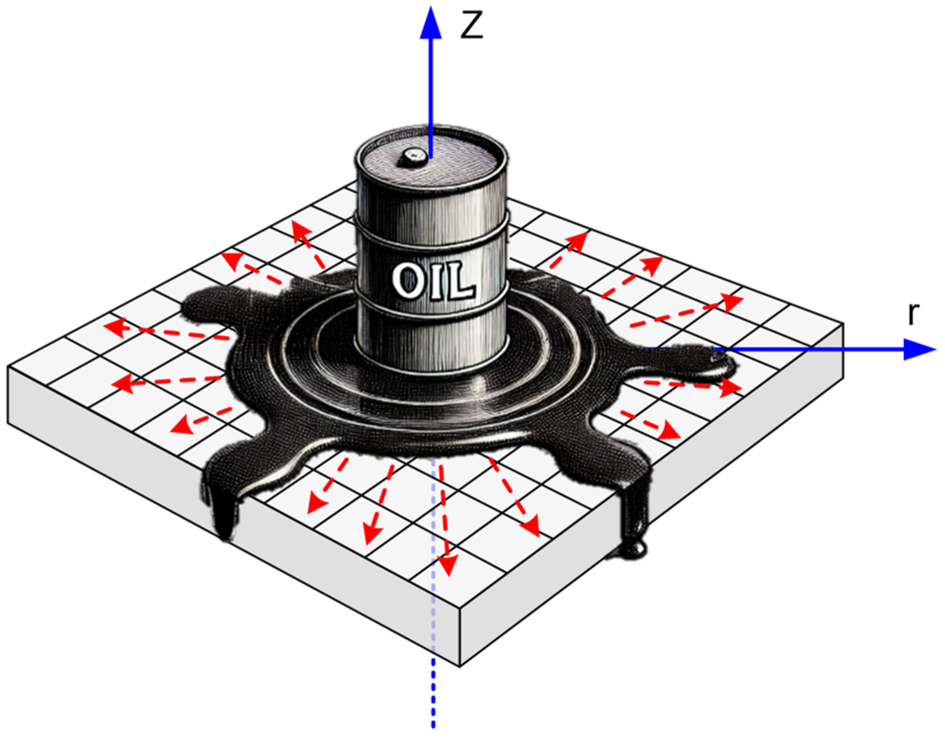
2.2. Diffusion of the Spilled Pollutant Problem and Derivation of Its Solution

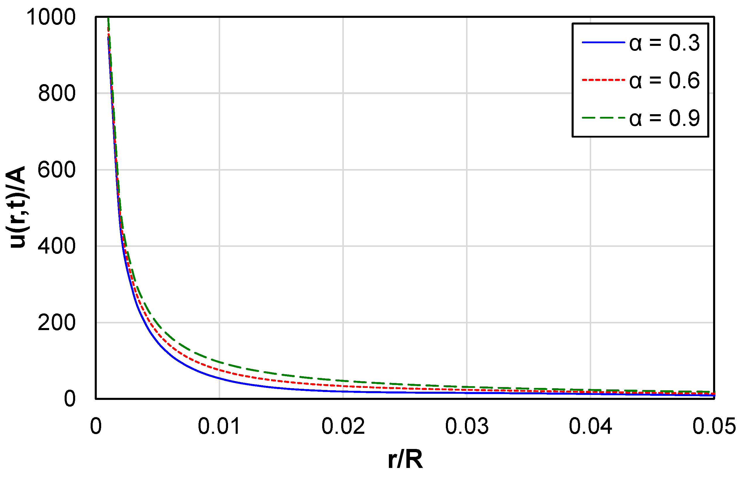
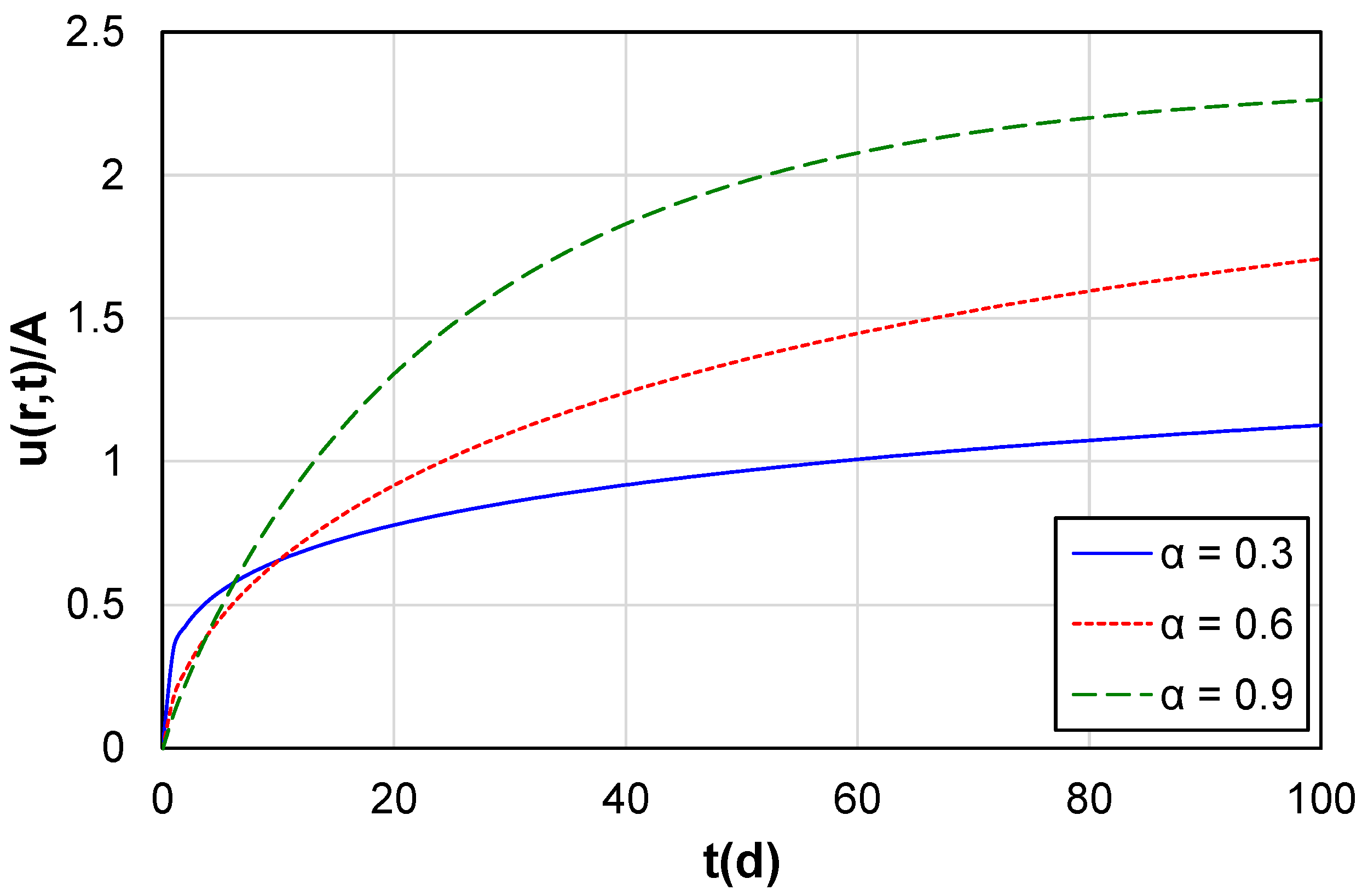
A pollutant is spilled and leaking into the ground as illustrated in Figure 1. The pollutant spill area on the ground is small enough to be assumed a point source. The diffusion problem is to be examined in spherical geometry. The pollutant density within the ground is assumed to be zero initially. Such a problem with ordinary time derivatives for a point pollutant source has already been examined [49].

The center of the leak area is taken to be the origin in the spherical coordinates. The soil is considered isotropic and homogeneous, and it is also assumed that it requires the conformable fractional derivative to be modeled properly. It is further assumed that the original ground spill was highly localized and spatially symmetric. Therefore, the symmetry requires that the concentration is independent of angular variables as shown below:

$${\displaystyle \frac{\partial u}{\partial \varphi }}=0$$

(5)

$${\displaystyle \frac{\partial u}{\partial \theta }}=0$$

(6)

$${\displaystyle \frac{{\partial }^{2}u}{\partial {\theta }^2}}=0$$

(7)

Therefore, the pollutant concentration depends only on time, $t$, and the radial distance, r, into the ground from the point of spill:

$$u=u\left(r,t\right)$$

(8)

Then, the analytical model for the pollutant concentration becomes

$${\displaystyle \frac{{\partial }^{\alpha }u\left(t\right)}{\partial t^{\alpha }}}={\displaystyle \frac{\partial u}{\partial t}}{t}^{1-\alpha }=D_{\alpha }\Delta u={\displaystyle \frac{D_{\alpha }}{r^2}}{\displaystyle \frac{\partial }{\partial r}}\left(r^2{\displaystyle \frac{\partial u}{\partial r}}\right)$$

(9)

where r is the radial distance into the ground from the spill point.

Equation (9), which is a partial differential equation, contains an integer order differential equation at each side due to the definition of the CFD being simpler than FDs such as the Caputo. The solution of this equation can be obtained using the method of separation of variables. Let $u=u\left(r, t\right)=X\left(r\right) T\left(t\right)$, where $X\left(r\right)$ is only the function of $r$ and $T\left(t\right)$ is only the function of $t$, and substitute it into the equation:

$${\displaystyle \frac{\partial u}{\partial t}}{t}^{1-\alpha }=D_{\alpha }\left({\displaystyle \frac{1}{r^2}}{\displaystyle \frac{\partial }{\partial r}}\left(r^2{\displaystyle \frac{\partial u}{\partial r}}\right)\right)=X{\displaystyle \frac{dT}{dt}}{t}^{1-\alpha }=D_{\alpha }\left({\displaystyle \frac{1}{r^2}}{\displaystyle \frac{\partial }{\partial r}}\left(r^2{\displaystyle \frac{dX}{dr}}T\right)\right)$$

(10)

$$X{\displaystyle \frac{dT}{dt}}{t}^{1-\alpha }=D_{\alpha }\left({\displaystyle \frac{1}{r^2}}\left[2r{X}^{\prime } T+r^2{X}^{″} T\right]\right)$$

(11)

$$X{\displaystyle \frac{dT}{dt}}{t}^{1-\alpha }=D_{\alpha }\left({\displaystyle \frac{2}{r}}{X}^{\prime } T+X^{″} \mathrm{T}\right)$$

(12)

When the equation is divided by X(r)T(t),

$${\displaystyle \frac{T^{\prime }}{T}}{ t}^{1-\alpha }=D_{\alpha }\left({\displaystyle \frac{2}{r}}{\displaystyle \frac{X^{\prime }}{X}}+{\displaystyle \frac{X^{″}}{X}} \right)$$

(13)

or

$${\displaystyle \frac{X^{″}}{X}}+{\displaystyle \frac{2}{r}}{\displaystyle \frac{X^{\prime }}{X}}={\displaystyle \frac{T^{\prime }}{T}} {\displaystyle \frac{t^{1-\alpha }}{D_{\alpha }}}=\mu$$

(14)

if $\mu ={\lambda }^2$,

$${\displaystyle \frac{X^{″}}{X}}+{\displaystyle \frac{2}{r}}{\displaystyle \frac{X^{\prime }}{X}}={\displaystyle \frac{T^{\prime }}{T}} {\displaystyle \frac{t^{1-\alpha }}{D_{\alpha }}}={\lambda }^2$$

(15)

When the first part of the above equation is solved, we have

$${\displaystyle \frac{X^{″}}{X}}+{\displaystyle \frac{2}{r}}{\displaystyle \frac{X^{\prime }}{X}}={\lambda }^2$$

(16)

if both sides of the equation are multiplied by $r^{2}X$, then

$$r^2{X}^{″}+2r{X}^{\prime }=r^2{\lambda }^2$$

(17)

or

$$r^2{X}^{″}+2r{X}^{\prime }-r^2{\lambda }^{2}X=0$$

(18)

Considering the values $\mu$ can take, there are three possible cases (Case 1, Case 2, and Case 3) to be considered. For Case 1, let us take $\mu ={\lambda }^2=0$. In this case, the following equation should be solved for $X_0$:

$$r^2{X}_0^{″}+2r{X}_0^{\prime }=0$$

(19)

If the last equation is divided by $r^2$, $\left(\mathrm{for} r\ne 0\right)$

$$X_0^{″}+{\displaystyle \frac{2}{r}}{X}_0^{\prime }=0$$

(20)

Solving this equation, we obtain

$${\displaystyle \frac{\frac{d^2{X}_0}{d{r}^2}}{2\frac{d{X}_0}{dr}}}=-{\displaystyle \frac{1}{r}} \Rightarrow {\displaystyle \frac{\frac{d^2{X}_0}{d{r}^2}dr}{2\frac{d{X}_0}{dr}}}=-{\displaystyle \frac{1}{r}}dr$$

(21)

Also, it is known that

$$d\left({\displaystyle \frac{d{X}_0}{dr}}\right)=d{X}_0^{\prime }$$

(22)

Submitting Equation (22) into Equation (21),

$${\displaystyle \frac{d{X}_0^{\prime }}{2X_0^{\prime }}}=-{\displaystyle \frac{dr}{r}}$$

(23)

By integrating both sides of Equation (23),

$$\int {\displaystyle \frac{d{X}_0^{\prime }}{2X_0^{\prime }}}=\int -{\displaystyle \frac{1}{r}}dr$$

(24)

The solution for $\mu ={\lambda }^2=0$ is obtained as follows:

$${\displaystyle \frac{1}{2}}\mathit{ln}{X}_0^{\prime }=-\mathit{ln}r+\mathit{ln}c$$

(25)

where $\mathit{ln}c$ is the integral constant. Using the properties of the logarithm and some algebraic operations, Equation (26) is given as follows:

$$X_0^{\prime }={\displaystyle \frac{c^2}{r^2}}$$

(26)

Renaming $c^2=c_1$, then

$$X_0^{\prime }={\displaystyle \frac{c_1}{r^2}}$$

(27)

When both sides of the last equation are integrated, the solution becomes

$$X_0=\int {\displaystyle \frac{c_1}{r^2}}dr=-{\displaystyle \frac{c_1}{r}}+c_2$$

(28)

For $\mu =0$ (Case 1), considering the time-dependent part of the differential equation,

$$\mu =0 \Rightarrow {\displaystyle \frac{d{T}_0}{dt}} {\displaystyle \frac{t^{1-\alpha }}{T_0{D}_{\alpha }}}=0$$

(29)

then,

$${\displaystyle \frac{d{T}_0}{dt}}=0$$

(30)

Next, the result is obvious that

$$T_0\left(t\right)=c_3$$

(31)

By multiplying $X_0\left(r\right)$ and $T_0\left(t\right)$, the solution of $u_0\left(r,t\right)$ for $\mu =0$ is found as follows:

$$u_0\left(t\right)=X_0\left(r\right)T_0\left(t\right)=\left(-{\displaystyle \frac{c_1}{r}}+c_2\right)c_3=C_2-{\displaystyle \frac{C_1}{r}}$$

(32)

where $C_2=c_2{c}_3$ and $C_1=c_1{c}_3$. Therefore, for $\lambda =0$ or $\mu =0$, the solution is found in Equation (33):

$$u_0=C_2-{\displaystyle \frac{C_1}{r}}$$

(33)

In the second case (Case 2), for $\mu ={\lambda }^2>0$,

$$r^2{X}_1^{″}+2r{X}_1^{\prime }-r^2{\lambda }^2{X}_1=0$$

(34)

or,

$$r{X}_1^{″}+2X_1^{\prime }-r{\lambda }^2{X}_1=0$$

(35)

This equation is called the Emden-Fowler Equation [50,51], and its solution is given below:

$$X_1\left(r\right)={\displaystyle \frac{k_1 e^{-\sqrt{\mu } r}}{r}}+{\displaystyle \frac{k_{2 }{e}^{\sqrt{\mu } r}}{\sqrt{\mu } r}}$$

(36)

where $k_1$ and $k_{2 }$ are integration constants. However, in the second case, for $\mu ={\lambda }^2>0$, the time-dependent part of Equation (15) is shown as follows:

$${\displaystyle \frac{T_1^{\prime }}{T_1}} {\displaystyle \frac{t^{1-\alpha }}{D_{\alpha }}}=\mu , \left(D_{\alpha }\ne 0\right)$$

(37)

$${\displaystyle \frac{T_1^{\prime }}{T_1}} {\displaystyle \frac{t^{1-\alpha }}{D_{\alpha }}}=\mu >0$$

(38)

Its solution can be obtained as follows:

$${\displaystyle \frac{t^{1-\alpha }\frac{d{T_1}^{\prime }}{dt}}{D_{\alpha }{T}_1}}=\mu$$

(39)

From here, ${T_1}^{\prime }$ is obtained so that

$${T_1}^{\prime }=D_{\alpha }\mu t^{\alpha -1}{T}_1$$

(40)

Let us divide Equation (40) by $T$:

$${\displaystyle \frac{T_1^{\prime }}{T_1}}=D_{\alpha }\mu t^{\alpha -1}$$

(41)

By taking the integral with respect to t on both sides,

$$\int {\displaystyle \frac{T_1^{\prime }}{T_1}} dt=D_{\alpha }\mu \int t^{\alpha -1}dt$$

(42)

Hence, the solution is found as below:

$$T_1\left(t\right)=c_4{e}^{ \left({\displaystyle \frac{D_{\alpha }\mu { t}^{\alpha }}{\alpha }}\right)}$$

(43)

Returning to the main equation and combining both solutions, the solution for $\mu >0$ is found in Equation (44):

$$\begin{array}{cc}{u}_1\left(r, t\right)=& X_1\left(r\right) T_1\left(t\right)=\left({\displaystyle \frac{k_1 e^{-\sqrt{\mu } r}}{r}}+{\displaystyle \frac{k_{2 }{e}^{\sqrt{\mu } r}}{\sqrt{\mu } r}}\right)c_4{e}^{ \left({\displaystyle \frac{D_{\alpha }\mu { t}^{\alpha }}{\alpha }}\right)}\\ & =\left({\displaystyle \frac{K_1 e^{-\sqrt{\mu } r}}{r}}+{\displaystyle \frac{K_{2 }{e}^{\sqrt{\mu } r}}{\sqrt{\mu } r}}\right)e^{ \left({\displaystyle \frac{D_{\alpha }\mu { t}^{\alpha }}{\alpha }}\right)}\end{array}$$

(44)

where $K_{1 }=k_1{c}_4$ and $K_{2 }=k_{2 }{c}_4$. The solution is not physical for $\mu >0$ since $U\left(r, t\right)$ goes to infinity as $t$ goes to infinity. At $r=R$, $u$ should be zero, and this condition can only be satisfied if $K_1$ and $K_2$ are equal to zero. Therefore,

$$u_1\left(r, t\right)=0$$

(45)

In the third case (Case 3), for $\lambda >0$ and $\mu =-{\lambda }^2<0$, the solution can be found by using different integration constants A and B and replacing $\mu =-{\lambda }^2$ in Equation (44). The solution is found as follows:

$$u_2\left(r, t\right)=\left({\displaystyle \frac{A e^{-\sqrt{\mu } r}}{r}}+{\displaystyle \frac{B{e}^{\sqrt{\mu } r}}{\sqrt{\mu } r}}\right)e^{ -\left({\displaystyle \frac{D_{\alpha }\mu { t}^{\alpha }}{\alpha }}\right)}$$

(46)

Since $\mu =-{\lambda }^2$, and remembering $j=\sqrt{-1}$,

$$\lambda =j\sqrt{\mu }$$

(47)

If $\lambda$ is different from and less than zero, Equation (47) turns into the following equations:

$$u_2\left(r,t\right)=\left({\displaystyle \frac{A{\mathrm{e}}^{-j\sqrt{\mu }r}}{r}}+{\displaystyle \frac{B{\mathrm{e}}^{j\sqrt{\mu }r}}{j\sqrt{\mu }r}}\right){\mathrm{e}}^{-\left({\displaystyle \frac{D_{\alpha }\mu t^{\alpha }}{\alpha }}\right)}$$

(48)

$$u_2\left(r,t\right)=\left({\displaystyle \frac{A{\mathrm{e}}^{-j\lambda r}}{r}}+{\displaystyle \frac{B{\mathrm{e}}^{j\lambda r}}{j\lambda r}}\right){\mathrm{e}}^{-\left({\displaystyle \frac{D_{\alpha }\mu t^{\alpha }}{\alpha }}\right)}$$

(49)

$$u_2\left(r,t\right)=\left({\displaystyle \frac{A{\mathrm{e}}^{-j\lambda r}}{r}}-{\displaystyle \frac{jB{\mathrm{e}}^{j\lambda r}}{\lambda r}}\right){\mathrm{e}}^{-\left({\displaystyle \frac{D_{\alpha }\mu t^{\alpha }}{\alpha }}\right)}$$

(50)

Equation (50) does not go to infinity when time goes to infinity. Therefore, it is a physical solution. However, it is not a unique solution. There may be an infinite number of $\lambda$ values (${\lambda }_n$) and an infinite number of solutions of $u_2\left(r,t\right)$, and the total solution can be given as the sum of all solutions:

$$u_2\left(r,t\right)={\displaystyle \sum }_{n=1}^{\infty }\left({\displaystyle \frac{A_n{\mathrm{e}}^{-j{\lambda }_{n}r}}{r}}-{\displaystyle \frac{j{B}_n{\mathrm{e}}^{j{\lambda }_{n}r}}{{\lambda }_{n}r}}\right){\mathrm{e}}^{-\left({\displaystyle \frac{D_{\alpha }\mu t^{\alpha }}{\alpha }}\right)}$$

(51)

The total solution of the DE is the sum of its solutions for Case 1 and Case 3:

$$u\left(r,t\right)=u_0\left(r,t\right)+u_2\left(r,t\right)$$

(52)

$$u\left(r,t\right)=u_o\left(r,t\right)+u_2\left(r,t\right)=C_2-{\displaystyle \frac{C_1}{r}}+{\displaystyle \sum }_{n=1}^{\infty }\left({\displaystyle \frac{A_n{\mathrm{e}}^{-j{\lambda }_{n}r}}{r}}-{\displaystyle \frac{j{B}_n{\mathrm{e}}^{j{\lambda }_{n}r}}{{\lambda }_{n}r}}\right){\mathrm{e}}^{-\left({\displaystyle \frac{D_{\alpha }\mu t^{\alpha }}{\alpha }}\right)}$$

(53)

Using the Euler formula $\left(e^{i\theta }=\cos \theta +i\sin \theta \right)$, Equation (53) turns into the following equation:

$$u\left(r,t\right)=C_2-{\displaystyle \frac{C_1}{r}}+{{\displaystyle \sum }}_{n=1}^{\infty }\left({\displaystyle \frac{A_n\left(\cos \left({\lambda }_{n}r\right)+i.\sin \left({\lambda }_{n}r\right)\right)}{r}}-{\displaystyle \frac{i{B}_n\left(\cos \left({\lambda }_{n}r\right)-i.\sin \left({\lambda }_{n}r\right)\right)}{{\lambda }_{n}r}}\right){\mathrm{e}}^{-\left({\displaystyle \frac{D_{\alpha }\mu t^{\alpha }}{\alpha }}\right)}$$

(54)

By rearranging the coefficients, Equation (54) turns into Equation (55):

$$u\left(r,t\right)=C_2-{\displaystyle \frac{C_1}{r}}+{{\displaystyle \sum }}_{n=1}^{\infty }{\displaystyle \frac{E_n\cos \left({\lambda }_{n}r\right)+F_n\sin \left({\lambda }_{n}r\right)}{r}}{\mathrm{e}}^{-\left({\displaystyle \frac{D_{\alpha }\mu t^{\alpha }}{\alpha }}\right)}$$

(55)

where the $E_n=A_n-{\displaystyle \frac{i{B}_n}{{\lambda }_n}}$ and $F_n=A_n-{\displaystyle \frac{B_n}{{\lambda }_n}}$.

The rate of the pollutant mass entering the ground is assumed to be constant. Initially, the soil was unpolluted; hence, the initial pollutant concentration within the ground is equal to zero:

$$u(r, 0)=0$$

(56)

At far distances from the point of pollution, the pollutant density can also be assumed to be zero for all time:

$$u(R, t)=0$$

(57)

${\lambda }_n$ is an eigenvalue for Equation (55). By taking ${\lambda }_n={\displaystyle \frac{n\pi }{R}}$, both boundary conditions, $u\left(R,0\right)=0$ and $u\left(0,t\right)=0$, must be satisfied. Therefore, at $t=0$ and $R=0$,

$$u\left(R,t\right)=C_2-{\displaystyle \frac{C_1}{R}}+{{\displaystyle \sum }}_{n=1}^{\infty }{\displaystyle \frac{E_n\cos \left(\frac{n\pi }{R}R\right)+F_n\sin \left(\frac{n\pi }{R}R\right)}{R}}{\mathrm{e}}^{-\left({\displaystyle \frac{D_{\alpha }\mu 0^{\alpha }}{\alpha }}\right)}=0$$

(58)

$$u\left(R,t\right)=C_2-{\displaystyle \frac{C_1}{R}}+{{\displaystyle \sum }}_{n=1}^{\infty }{\displaystyle \frac{E_n\cos \left(n\pi \right)+F_n\sin \left(n\pi \right)}{R}}{\mathrm{e}}^0=C_2-{\displaystyle \frac{C_1}{R}}+{{\displaystyle \sum }}_{n=1}^{\infty }{\displaystyle \frac{E_n}{R}}=0$$

(59)

Hence, the following conditions must be satisfied:

$$E_n=0$$

(60)

and

$$C_2-{\displaystyle \frac{C_1}{R}}=0$$

(61)

Therefore,

$$C_2={\displaystyle \frac{C_1}{R}}$$

(62)

Equation (55) turns into the following equation:

$$u\left(r,t\right)={\displaystyle \frac{C_1}{R}}-{\displaystyle \frac{C_1}{r}}+{\displaystyle \frac{{{\displaystyle \sum }}_{n=1}^{\infty }{F}_n\sin \left({\lambda }_{n}r\right){\mathrm{e}}^{-\left(\frac{D_{\alpha }\mu t^{\alpha }}{\alpha }\right)}}{r}}$$

(63)

Taking the partial derivative of the Equation (63) with respect to $r$:

$${\displaystyle \frac{\partial u\left(r,t\right)}{\partial r}}={\displaystyle \frac{C_1}{r^2}}+{\displaystyle \frac{{{\displaystyle \sum }}_{n=1}^{\infty }{\lambda }_n{F}_n(\cos \left({\lambda }_{n}r\right)r-\sin \left({\lambda }_{n}r\right)){\mathrm{e}}^{-\left(\frac{D_{\alpha }\mu t^{\alpha }}{\alpha }\right)}}{r^2}}$$

(64)

Since the pollutant source is assumed to be a point source, the conservation of mass law or the continuity equation requires that

$$2\mathsf{\pi }k\underset{r\to 0}{\mathit{lim}} \left(r^2{\displaystyle \frac{\partial u(r,t)}{\partial r}}\right)=-{\displaystyle \frac{dm}{dt}}$$

(65)

where ${\displaystyle \frac{dm}{dt}}$ is the rate of the pollutant mass entering the ground and $k$ is the permeability of the earth to this compound. Submitting Equation (64) into Equation (65),

$$2\mathsf{\pi }k\underset{r\to 0}{\mathit{lim}}\left(r^2\left({\displaystyle \frac{C_1}{r^2}}+{\displaystyle \frac{{{\displaystyle \sum }}_{n=1}^{\infty }{\lambda }_n{F}_n(\cos \left({\lambda }_{n}r\right)r-\sin \left({\lambda }_{n}r\right)){\mathrm{e}}^{-\left(\frac{D_{\alpha }\mu t^{\alpha }}{\alpha }\right)}}{r^2}}\right)\right)=-{\displaystyle \frac{dm}{dt}}$$

(66)

$$2\mathsf{\pi }k\underset{r\to 0}{\mathit{lim}}\left(C_1+{\displaystyle \sum }_{n=1}^{\infty }{\lambda }_n{F}_n(\cos \left({\lambda }_{n}r\right)r-\sin \left({\lambda }_{n}r\right)){\mathrm{e}}^{-\left({\displaystyle \frac{D_{\alpha }\mu t^{\mathsf{\alpha }}}{\alpha }}\right)}\right)=-{\displaystyle \frac{dm}{dt}}$$

(67)

$$2\mathsf{\pi }k\left(C_1+{\displaystyle \sum }_{n=1}^{\infty }{\lambda }_n{F}_n(\cos \left(0\right).0-\sin (0){\mathrm{e}}^{-\left({\displaystyle \frac{D_{\alpha }\mu t^{\alpha }}{\alpha }}\right)}\right)=-{\displaystyle \frac{dm}{dt}}$$

(68)

$$2\mathsf{\pi }k{C}_1=-{\displaystyle \frac{dm}{dt}}$$

(69)

$$\dot{m}={\displaystyle \frac{dm}{dt}}=-2\pi k{C}_1$$

(70)

$$C_1=-{\displaystyle \frac{\dot{m}}{2\pi k}}$$

(71)

Equation (55) turns into

$$u\left(r,t\right)={\displaystyle \frac{C_1}{R}}-{\displaystyle \frac{C_1}{r}}+{\displaystyle \frac{{{\displaystyle \sum }}_{n=1}^{\infty }{F}_n\sin \left(\frac{n\pi }{R}r\right){\mathrm{e}}^{-\left(\frac{D_{\alpha }\mu t^{\alpha }}{\alpha }\right)}}{r}}$$

(72)

$$u\left(r,t\right)={\displaystyle \frac{C_1}{R}}-{\displaystyle \frac{C_1-{{\displaystyle \sum }}_{n=1}^{\infty }{F}_n\sin \left(\frac{n\pi }{R}r\right){\mathrm{e}}^{-\left(\frac{D_{\alpha }\mu t^{\alpha }}{\alpha }\right)}}{r}}$$

(73)

$$u\left(r,t\right)={\displaystyle \frac{C_{1}r-R{C}_1-{{\displaystyle \sum }}_{n=1}^{\infty }R{F}_n\sin \left(\frac{n\pi }{R}r\right){\mathrm{e}}^{-\left(\frac{D_{\alpha }\mu t^{\alpha }}{\alpha }\right)}}{\mathit{Rr}}}$$

(74)

At t = 0, the initial pollutant distribution within the soil is zero. Therefore, the following is true: at $t=0$. Considering $u (r, 0)=0,$ the nominator should also be zero at $t=0$:

$$C_{1}r-R{C}_1-{\displaystyle \sum }_{n=1}^{\infty }R{F}_n\sin \left({\displaystyle \frac{n\pi }{R}}r\right){\mathrm{e}}^0=0$$

(75)

This means that for $0<r<R$

$$C_{1}r-R{C}_1={\displaystyle \sum }_{n=1}^{\infty }R{F}_n\sin \left({\displaystyle \frac{n\pi }{R}}r\right)$$

(76)

Any function can be represented as a Fourier series. In the range of $-R<r<R$, let us assume that the ${{\displaystyle \sum }}_{n=1}^{\infty }R{F}_n\sin \left({\displaystyle \frac{n\pi }{R}}r\right)$ is an odd function due to the sinusoidal terms with a period of $2R$. Its equation can be written as

$${\displaystyle \sum }_{n=1}^{\infty }R{F}_n\sin \left({\displaystyle \frac{n\pi }{R}}r\right)=\left\{\begin{array}{cc}{C}_{1}r-R{C}_1 ,& 0<r<R\\ -C_{1}r+R{C}_1 ,& -R<r<0\end{array}\right.$$

(77)

Its Fourier series coefficients are found as follows:

$$R{F}_n=2{\displaystyle \frac{2}{2R}}{{\displaystyle \int }}_{r=0}^{r=R}u\left(r,0\right)\sin \left({\displaystyle \frac{n\pi }{R}}r\right)dr$$

(78)

$$R{F}_n={\displaystyle \frac{2}{R}}{{\displaystyle \int }}_{r=0}^{r=R}\left(C_{1}r-R{C}_1\right)\sin \left({\displaystyle \frac{n\pi }{R}}r\right)dr$$

(79)

$$R{F}_n=-{\displaystyle \frac{2}{R}}{\displaystyle \frac{\left(R{C}_1\right)}{\left(\frac{n\pi }{R}\right)}}=-{\displaystyle \frac{2R{C}_1}{n\pi }}$$

(80)

Therefore,

$$R{F}_n=-{\displaystyle \frac{2R{C}_1}{n\pi }}$$

(81)

Thus, the sought solution is found below:

$$u\left(r,t\right)={\displaystyle \frac{C_{1}r-R{C}_1-{{\displaystyle \sum }}_{n=1}^{\infty }\left(-\frac{2R{C}_1}{n\pi }\right)\sin \left(\frac{n\pi }{R}r\right)e^{-\left(\frac{D_{\alpha }\mu t^{\alpha }}{\alpha }\right)}}{\mathit{Rr}}}$$

(82)

$$u\left(r,t\right)={\displaystyle \frac{C_{1}r-R{C}_1+{{\displaystyle \sum }}_{n=1}^{\infty }\left(\frac{2R{C}_1}{n\pi }\right)\sin \left(\frac{n\pi }{R}r\right)e^{-\left(\frac{D_{\alpha }\mu t^{\alpha }}{\alpha }\right)}}{\mathit{Rr}}}$$

(83)

Substituting $C_1=-{\displaystyle \frac{\dot{m}}{2\pi k}}$, $C_2$ and $\lambda ={\displaystyle \frac{\pi }{R}}$ into Equation (83), we obtain

$$u\left(r,t\right)=-{\displaystyle \frac{\dot{m}}{2\pi k}}\left({\displaystyle \frac{r-R+{{\displaystyle \sum }}_{n=1}^{\infty }\left(\frac{2R}{n\pi }\right)\sin \left(\frac{n\pi }{R}r\right)e^{-\left(\frac{D_{\alpha }\mu t^{\alpha }}{\alpha }\right)}}{\mathit{Rr}}}\right)$$

(84)

3. Results

A program was written in Matlab^TM (https://www.mathworks.com/products/matlab.html) to simulate the pollutant problem. The simulation results are shown in Figure 2 and Figure 3. The normalized pollutant concentration as a function of the normalized radius $\left(r/R\right)$ is given in Figure 2 for three different α values.

The concentration of the pollutant decreases from the spill point into the earth. The pollutant density is much higher just under the spill and falls rapidly further away from it. The normalized pollutant concentration curves converge at low values of $\left(r/R\right)$ since the term $\left(1/r\right)$ becomes dominant, resulting in an almost hyperbolic behavior. It appears to fall to zero when the pollutant diffuses further into the earth and the three different curves start asymptotically converging.

The normalized pollutant concentration as a function of time is presented in Figure 3 for three different α values at $r/R=0$.

The pollutant concentration increases with increasing time due to the non-zero rate of the pollutant mass entering the ground since the initial pollutant concentration was zero. Remarkably, higher orders of the conformal derivative lead to larger contamination concentration profiles when time increases beyond 10 days, while lower orders of the conformal derivative lead to larger contamination concentration profiles when time is less than 3 days. This can be explained by the term $e^{-\left({\displaystyle \frac{D_{\alpha }\mu t^{\alpha }}{\alpha }}\right)}$ behaving differently considering the $t^{\alpha }$ term. Its dynamics are governed by the order of CFD and the increasing time. Importantly, the observed curves do not follow an exponential trend, since α is not equal to 1. As the order of CFD increases, the type of the diffusion process changes gradually from sub-diffusion to normal diffusion.

4. Discussion

Diffusion is a three-dimensional problem. It is impossible to obtain solutions to each three-dimensional problem analytically. However, the diffusion problem with a spherical symmetry examined here yielded an analytical solution. Such a solution may not be possible without using more sophisticated techniques such as the green function approach with well-known fractional derivatives like Caputo [52]. The solution given here can easily be modified for the spherically symmetric problems with different boundary conditions. The solution given here can also be applied to the heat transfer problems describable with similar equations. In this problem, a point pollutant source is assumed. If the source has a considerable surface, a numerical method such as the finite difference time domain method may be utilized for the solutions. The solution given here can be applied to pollutant problems with an almost point source to see whether the CFD is usable to describe the pollutant diffusion in the concerned soil or not. Also, examining the pollutant concentration in the near field of the point source, the order of the conformal fractional derivative cannot be determined since there is an almost hyperbolic behavior. However, by taking polluted soil samples in several places away from the point-like source within the ground at different times, it may be possible to define the order of the CFD and the generalized diffusion coefficient D_α.

It is well known that the Fourier series converges at every point where the function is continuous [49,53]. Equation (77) represents a sawtooth waveform. Except for the discontinuity at $r=0$, practically everywhere its Fourier series converges pointwise to the function; nonetheless, because of the Gibbs phenomenon, it exhibits oscillating behavior at that point. A Fourier series converges to the average of the left-hand and right-hand limits [49,54]. Since their average is equal to zero as seen from Equation (77), the Fourier series of the solution converges to zero. This can also be observed from the fact that the sinusoidal terms, $\sin \left({\displaystyle \frac{n\pi }{R}}r\right),$ are zero at $r=0$. However, as $r$ approaches zero from the right-hand side, the numerator of Equation (81) approaches the value $-R{C}_1. u\left(r,t\right)$ diverges at $r=0$. It converges at all the other points where the function is continuous. It is well known that the Fourier series of the sawtooth wave overshoots the actual value by about 9% at the points of discontinuity, leading to an oscillatory behavior that does not disappear as more terms are added. However, the overshoot remains bounded, and this is a characteristic of the Fourier series representing discontinuous functions. At $r=0$, due to the $r$ term in the denominator, the $u\left(r,t\right)$ diverges. That is why the function should not be evaluated at around $r=0$. However, Equation (84) is the solution of the CFD-based diffusion equation, and it converges at all points away from the discontinuity at $r=0$ since the function is continuous.

5. Conclusions

The inspection of pollutants in soils is a significant issue. In recent years, studies on diffusion using fractional differential equations have gained popularity. Given that soil is not a homogeneous medium, diffusion problems in certain soils can be effectively modeled with fractional derivatives (FDs). This study analytically solved a CFD-based diffusion equation in three dimensions with complete symmetry, assuming constant soil permeability and temperature, and that the soil is isotropic and homogeneous. The solution was examined parametrically, considering the order of the CFD.

The method presented here can also be applied to pollution problems with various boundary conditions, such as irregular and inter-boundary conditions. A parametric analysis was conducted for different values of α. The solution of the CFD-based differential equation includes a stretched exponential term. For α = 1, the conformable diffusion equation simplifies to the traditional diffusion equation. Future work could examine anisotropic diffusion or diffusion without axisymmetric in spherical coordinates. The solution of the CFD-based differential equation has proven to be more practical, simple, and easily applicable than solutions using other fractional derivatives, such as Caputo or Riemann–Liouville. This solution can guide researchers working on conformable fractional differential equations and may serve as a useful tool for solving certain mathematical models. Given that soil is a heterogeneous medium, the technique presented in this study can be extended to more complex diffusion problems, potentially involving heterogeneous soil regions with inter-boundary and irregular boundary conditions.

References

1. Miller, K.S.; Ross, B. An Introduction to the Fractional Calculus and Fractional Differential Equations, 1st ed.; Wiley: Hoboken, NJ, USA, 1993. [Google Scholar]
2. Ross, B. The development of fractional calculus 1695–1900. Hist. Math. 1977, 4, 75–89. [Google Scholar] [CrossRef]
3. Podlubny, I. Fractional Differential Equations: An Introduction to Fractional Derivatives, Fractional Differential Equations, to Methods of Their Solution and Some of Their Applications, 1st ed.; Elsevier: Amsterdam, The Nederlands, 1998. [Google Scholar]
4. Samko, S.G.; Kilbas, A.A.; Marichev, O.I. Fractional Derivatives and Integrals: Theory and Applications; Gordon and Breach Science Publishers: Philadelphia, PA, USA, 1993. [Google Scholar]
5. Yang, X.J. General Fractional Derivatives: Theory, Methods and Applications, 1st ed.; Chapman and Hall/CRC: Boca Raton, FL, USA, 2019. [Google Scholar]
6. Su, N. Fractional Calculus for Hydrology, Soil Science and Geomechanics: An Introduction to Applications, 1st ed.; CRC Press: Boca Raton, FL, USA, 2020. [Google Scholar]
7. Babiarz, A.; Czornik, A.; Klamka, J.; Niezabitowski, M. Theory and applications of non-integer order systems. In Proceedings of the 8th Conference on Non-integer Order Calculus and Its Applications, Zakopane, Poland, 20–21 September 2016. [Google Scholar]
8. Kilbas, A.A.; Srivastava, H.M.; Trujillo, J.J. Theory and Applications of Fractional Differential Equations, 1st ed.; Elsevier: Amsterdam, The Nederlands, 2006. [Google Scholar]
9. Desai, C.S.; Zaman, M. Advanced Geotechnical Engineering: Soil-Structure Interaction Using Computer and Material Models; Taylor & Francis: London, UK, 2013. [Google Scholar]
10. Langlands, T.A.; Henry, B.I. The accuracy and stability of an implicit solution method for the fractional diffusion equation. J. Comput. Phys. 2005, 205, 719–736. [Google Scholar] [CrossRef]
11. Li, C.; Zeng, F. Numerical Methods for Fractional Calculus, 1st ed.; CRC Press: Boca Raton, FL, USA, 2015. [Google Scholar]
12. Tadjeran, C.; Meerschaert, M.M. A second-order accurate numerical method for the two-dimensional fractional diffusion equation. J. Comput. Phys. 2007, 220, 813–823. [Google Scholar] [CrossRef]
13. Aslefallah, M.; Rostamy, D.; Hosseinkhani, K. Solving time-fractional differential diffusion equation by theta-method. Int. J. Adv. Appl. Math. Mech. 2014, 2, 1–8. [Google Scholar]
14. Gong, C.; Bao, W.; Tang, G.; Jiang, Y.; Liu, J. A parallel algorithm for the two-dimensional time fractional diffusion equation with implicit difference method. Sci. World J. 2014, 2014, 219580. [Google Scholar] [CrossRef]
15. Pandey, P.; Kumar, S.; Gomez-Aguilar, J.F. Numerical solution of the time fractional reaction-advection-diffusion equation in porous media. J. Appl. Comput. Mech. 2022, 8, 84–96. [Google Scholar] [CrossRef]
16. Li, L.; Jiang, Z.; Yin, Z. Compact finite-difference method for 2D time-fractional convection-diffusion equation of groundwater pollution problems. Comput. Appl. Math. 2020, 39, 142. [Google Scholar] [CrossRef]
17. Atangana, A.; Kilicman, A. Analytical solutions of the space-time fractional derivative of advection dispersion equation. Math. Probl. Eng. 2013, 2013, 853127. [Google Scholar] [CrossRef]
18. Khalil, R.; Al Horani, M.; Yousef, A.; Sababheh, M. A new definition of fractional derivative. J. Comput. Appl. Math. 2014, 264, 65–70. [Google Scholar] [CrossRef]
19. Abdeljawad, T. On conformable fractional calculus. J. Comput. Appl. Math. 2015, 279, 57–66. [Google Scholar] [CrossRef]
20. Teodoro, G.S.; Machado, J.T.; De Oliveira, E.C. A review of definitions of fractional derivatives and other operators. J. Comput. Phys. 2019, 388, 195–208. [Google Scholar] [CrossRef]
21. Zhao, D.; Luo, M. General conformable fractional derivative and its physical interpretation. Calcolo 2017, 54, 903–917. [Google Scholar] [CrossRef]
22. Abu Hammad, I.; Khalil, R. Fractional fourier series with applications. Am. J. Comput. Appl. Math. 2014, 4, 187–191. [Google Scholar] [CrossRef]
23. Hammad, M.A.; Khalil, R. Legendre fractional differential equation and legender fractional polynomials. Int. J. Appl. Math. Res. 2014, 3, 214–219. [Google Scholar] [CrossRef]
24. Tajadodi, H.; Khan, Z.A.; Irshad, A.R.; Gomez-Aguilar, J.F.; Khan, A.; Khan, H. Exact solutions of conformable fractional differential equations. Results Phys. 2021, 22, 103916. [Google Scholar] [CrossRef]
25. Patel, H.; Patel, T.; Pandit, D. An efficient technique for solving fractional-order diffusion equations arising in oil pollution. J. Ocean Eng. Sci. 2023, 8, 217–225. [Google Scholar] [CrossRef]
26. Bouaouid, M.; Hilal, K.; Melliani, S. Nonlocal telegraph equation in frame of the conformable time-fractional derivative. Adv. Math. Phys. 2019, 2019, 7528937. [Google Scholar] [CrossRef]
27. Ortega, A.; Rosales, J.J. Newton’s law of cooling with fractional conformable derivative. Rev. Mex. Fís. 2018, 64, 172–175. [Google Scholar] [CrossRef]
28. Bayrak, M.A.; Demir, A.; Ozbilge, E. A novel approach for the solution of fractional diffusion problems with conformable derivative. Numer. Meth. Part Differ. Equ. 2023, 39, 1870–1887. [Google Scholar] [CrossRef]
29. Chaudhary, M.; Kumar, R.; Singh, M.K. Fractional convection-dispersion equation with conformable derivative approach. Chaos Solitons Fractals 2020, 141, 110426. [Google Scholar] [CrossRef]
30. Zhou, H.; Yang, S.; Zhang, S. Conformable derivative approach to anomalous diffusion. Physica A 2018, 491, 1001–1013. [Google Scholar] [CrossRef]
31. Sabaté, J.; Vinas, M.; Solanas, A. Laboratory-scale bioremediation experiments on hydrocarbon-contaminated soils. Int. Biodeterior. Biodegrad. 2004, 54, 19–25. [Google Scholar] [CrossRef]
32. Reible, D.; Demnerova, K. Innovative Approaches to the On-Site Assessment and Remediation of Contaminated Sites, 15th ed.; Springer: Berlin/Heidelberg, Germany, 2012. [Google Scholar]
33. Blazek, J. Computational Fluid Dynamics: Principles and Applications, 3rd ed.; Elsevier: Amsterdam, The Nederlands, 2015. [Google Scholar]
34. He, J.H. Approximate analytical solution for seepage flow with fractional derivatives in porous media. Comput. Meth. Appl. Mech. Eng. 1998, 167, 57–68. [Google Scholar] [CrossRef]
35. Ordu, S.; Ordu, E.; Mutlu, R. Axisymmetric spilled pollutant analysis in steady-state using finite difference method. Fresenius Environ. Bull. 2022, 31, 9587–9592. [Google Scholar]
36. Ordu, S.; Ordu, E.; Mutlu, R. Seepage analysis from a long-polluted river in steady-state using finite difference method. Adiyaman Univ. J. Eng. Sci. 2023, 10, 1–14. (In Turkish) [Google Scholar] [CrossRef]
37. Salehi, Y.; Darvishi, M.T.; Schiesser, W.E. Numerical solution of space fractional diffusion equation by the method of lines and splines. Appl. Math. Comput. 2018, 336, 465–480. [Google Scholar] [CrossRef]
38. Wang, Y.M.; Wang, T. A compact locally one-dimensional method for fractional diffusion-wave equations. J. Appl. Math. Comput. 2015, 49, 41–67. [Google Scholar] [CrossRef]
39. Zhang, K. Existence results for a generalization of the time-fractional diffusion equation with variable coefficients. Bound. Value Probl. 2019, 2019, 10. [Google Scholar] [CrossRef]
40. Zhuang, P.; Liu, F. Finite difference approximation for two-dimensional time fractional diffusion equation. J. Algorithms Comput. Technol. 2007, 1, 1–16. [Google Scholar] [CrossRef]
41. Murio, D.A. Implicit finite difference approximation for time fractional diffusion equations. Comput. Math. Appl. 2008, 56, 1138–1145. [Google Scholar] [CrossRef]
42. Baleanu, D.; Agheli, B.; Al Qurashi, M.M. Fractional advection differential equation within Caputo and Caputo–Fabrizio derivatives. Adv. Mech. Eng. 2016, 8, 1687814016683305. [Google Scholar] [CrossRef]
43. Bohaienko, V.; Bulavatsky, V. Mathematical modeling of solutes migration under the conditions of groundwater filtration by the model with the k-Caputo fractional derivative. Fractal Fract. 2018, 2, 28. [Google Scholar] [CrossRef]
44. Gulkaç, V. A method of finding source function for inverse diffusion problem with time-fractional derivative. Adv. Math. Phys. 2016, 2016, 6470949. [Google Scholar] [CrossRef]
45. Bildik, N.; Deniz, S. A new fractional analysis on the polluted lakes system. Chaos Solitons Fractals 2019, 122, 17–24. [Google Scholar] [CrossRef]
46. Yao, L.; Ren, L.; Gong, G. Time-fractional model of chloride diffusion in concrete: Analysis using meshless method. Adv. Mater. Sci. Eng. 2020, 2020, 4171689. [Google Scholar] [CrossRef]
47. Mirza, I.A.; Akram, M.S.; Shah, N.A.; Akhtar, S.; Muneer, M. Study of one-dimensional contaminant transport in soils using fractional calculus. Math. Meth. Appl. Sci. 2021, 44, 6839–6856. [Google Scholar] [CrossRef]
48. Atangana, A.; Bildik, N. The use of fractional order derivative to predict the groundwater flow. Math. Probl. Eng. 2013, 2013, 543026. [Google Scholar] [CrossRef]
49. MacCluer, C.R. Boundary Value Problems and Orthogonal Expansions: Physical Problems from a Sobolev Viewpoint, 1st ed.; IEEE Press: Piscataway, NJ, USA, 1994. [Google Scholar]
50. Wong, J.S. On the generalized Emden–Fowler equation. J. Korean Soc. Ind. Appl. Math. 1975, 17, 339–360. [Google Scholar] [CrossRef]
51. Emden, R. Gaskugeln, Anwendungen der Mechanischen Warmen-Theorie auf Kosmologie und Meteorologische Probleme, 1st ed.; Bibliotheca Teubneriana: Berlin, Germany, 1907. [Google Scholar]
52. Lucena, L.; Da Silva, L.; Evangelista, L.; Lenzi, M.; Rossato, R.; Lenzi, E. Solutions for a fractional diffusion equation with spherical symmetry using green function approach. Chem. Phys. 2008, 344, 90–94. [Google Scholar] [CrossRef]
53. Carleson, L. On convergence and growth of partial sums of Fourier series. Acta Math. 1966, 116, 135–157. [Google Scholar] [CrossRef]
54. Dirichlet, G.L. Sur la convergence des series trigonometriques qui servent à represénter une fonction arbitraire entre des limites donnees. J. Reine Angew. Math. 1829, 4, 157–169. [Google Scholar]
Figure 1. Pollutant problems in spherical coordinates.
Symmetry 16 01358 g001
Figure 2. Concentration profiles for different conformable derivative orders at t = 100 days, with D α μ = 0.05.
Symmetry 16 01358 g002
Figure 3. Diffusion curves for r = 0.3R with different conformable derivative orders.
Symmetry 16 01358 g003
Disclaimer/Publisher’s Note: The statements, opinions and data contained in all publications are solely those of the individual author(s) and contributor(s) and not of MDPI and/or the editor(s). MDPI and/or the editor(s) disclaim responsibility for any injury to people or property resulting from any ideas, methods, instructions or products referred to in the content.