A Discrete-Time Queueing Model of a Bottleneck with an Energy-Saving Mechanism Based on Setup and Shutdown Times

Abstract

Producers are encouraged to reduce their energy consumption of manufacturing systems by applying less-energy-intensive modern technologies and advanced machine tools and operating methods at the system level. In the paper, organizational and analytical solutions are combined to model the sustainable production system. Managers can study the behavior of a production system organized using energy-saving rules by changing key parameters of the input model (arrival intensity, bottleneck service rate, buffer size, setup and shutdown time) to analyze the queue size of the production system and therefore performance. A discrete-time queueing model of a single-bottleneck production line with a finite input buffer capacity is proposed. Jobs occur according to a binomial process and are processed individually, one by one, according to the natural FIFO service discipline, with a general discrete-type cumulative distribution function. The total number of jobs present in the system is bounded by a non-random fixed value N. Every time the system becomes empty, an energy-saving mechanism is started: the processing machine (server) is turned off during a geometrically distributed shutdown time. Similarly, the first job arriving into the empty system initializes a geometrically distributed setup time. Identifying renewal moments in the evolution of the model, a system of difference equations is built for the transient queue-size distribution conditioned by the state of the system at the opening. The solution is obtained explicitly in terms of probability-generating functions. In addition, the Drum-Buffer-Rope concept is proposed to reduce the energy consumption of the production line. The throughput of the production system is maximized by adjusting the time between the order arrivals and the size of the input buffer to the capacity of the bottleneck. Turning off a machine under certain conditions and slowing down non-critical machines are strategies to reduce energy consumption. A detailed illustrating numerical and simulation study of the considered model is attached as well, in which the sensitivity of the queue-size behavior to changes of the key input model parameters is investigated.

1. Introduction

The energy crisis is a very pressing problem due to the constant use of non-renewable energy sources and the greenhouse effect [1]. Solving the problems of sequencing and scheduling that focus on energy efficiency is a hot topic [2]. The accurate measurement of energy consumption during operation is necessary to minimize energy [3,4]. Due to rising energy prices, the reduction in energy consumption costs of production machines is the subject of much research [5]. Machines operate in different processing modes, consuming different levels of energy, which have different effects on the wear process of the machines [6].

Producers are encouraged to reduce their energy consumption of manufacturing systems by applying less-energy-intensive modern technologies and advanced machine tools or operating methods at the system level, such as energy-efficient scheduling (EES) [7]. In the related literature, various models of energy consumption processes by machines [5] and types of shop floors are analyzed. The models are classified according to computational complexity, such as scheduling individual machines [8,9,10,11,12,13], flow shops [1,2,6,14,15], job shops [16,17,18], and flexible job shops [19], as well as hybrid systems for specific issues [20,21,22]. No-wait flow shop scheduling is a hot topic in academic research due to its wide applicability in industrial domains [6]. Including energy-efficient scheduling, the complexity of the last problem is $n!L^{nl}$, where n, l and L are numbers of the production tasks, machines and speed grades of the machines, respectively. Flow shop planning problems are popular because more than 25% of production systems, assembly lines and information services can be simplified to a flow shop problem [23]. No-wait flow shop energy-efficient scheduling is rarely studied in academic research [2,6].

In the case of many machine tools, the power consumption at idle is only slightly lower than the power consumption during operation [24]. Studies show that shutting down the idle machine is a common measure that is appropriate for all types of workshops [24] but requires more setup and shutdown operations than usual [25,26], which makes management difficult. Grouping different jobs into the batches and starting the production for the sequenced batches called the blocking permutation flow shop scheduling problem is also the strategy for energy cost reduction [27]. A batch stays on the machine after processing until the next machine is available. Optimization of the machine amount for each job in the distributed flow shop is proposed in [28]. For efficient energy consumption, the energy consumption is analyzed not only during processing but also in the idle and setup states [28]. In order to reduce processing, idle, and turnoff energy consumption, jobs are processed in parallel in the first stage, and once assigned to a single batch, the batch is processed in the second stage [14]. Of course, batch production involves more operational and practical decisions, especially regarding how to form a batch when starting batch processing [14].

Researchers also include time-dependent energy costs, such as time-of-use electricity tariffs, as well as machine-based energy charges, such as processing, idle, setup and close-down times [27,28]. The energy consumption is minimized based on the power consumption of each machine, which is known and deterministic [29]. A very interesting approach is to optimize the machine processing speed of non-critical operations from three possible levels of operation: slow, fast and normal is proposed in [6,30]. Reducing the processing speed of non-critical operations reduces energy consumption without compromising the makespan. An energy-efficient permutation flow shop with sequence-dependent setup times and transportation times is presented in [22]. However, transportation times can be analyzed as operation times in flow shop problems.

The simplest mechanism for saving energy is to turn the machine off [15] if it has been waiting for a relatively long time for a new job and then restart it when a new job is available. When sequencing and selecting the size of a production batch, it is necessary to analyze whether it is worth waiting for a certain number of tasks to accumulate in the finite-capacity input buffer and releasing the batch at the right time to production to save energy and complete tasks on time. Production in batches (repetitive) is popular, an example being the automotive industry, but it is often overlooked in the flow problems under consideration. The method of waiting (on the Kanban board) for the required number of batches of a given type of product in the Kanban card control is known and common [31], but energy-efficient analysis is strongly needed. Only a few examples of the flow shop energy-efficient scheduling problem for a given batch size for serial flow, parallel flow [27,32], and serial–parallel flow [33] are available in the related literature.

Taking into account the literature review, the research gap is related to the setup and shutdown activities associated with more frequent machine starts and shutdowns, which are often overlooked. A batch size analysis is definitely needed for energy-efficient sequencing and planning.

Enterprises try to minimize the number of orders lost due to input buffer overflow by maximizing machine utilization. Increasing the processing capacity of machines and devices for timely production increases energy consumption. Sustainable production requires energy-efficient production, so optimization is key. Predicting the sojourn time (waiting time + processing time) of a queued job helps to decide whether to accept a new job and to plan production resources with limited capacity. Estimating the actual sojourn time of production tasks should take into account the analysis of two objectives: energy-efficient and timely production.

The use in the considered model of an energy-saving mechanism based on temporarily turning off the machine and the associated setup and shutdown periods allows for achieving a certain symmetry in the effective use of the machine. On the one hand, obvious benefits are achieved in terms of reducing the costs of system operation (during the period when the machine is turned off). On the other hand, these periods can be used for additional activities: checking the machine’s efficiency, installing additional components, etc. Therefore, although no tasks are handled during the setup/closedown periods, which results in a temporary extension of the queue, after a restart, the machine is, for example, better prepared for possible failures and disruptions.

The analyzed studies show that the improvement of energy efficiency when using EES is significant. The goal is to develop a research framework for energy-efficient planning using an original discrete simulation model for queueing analysis. A production model including the Drum-Buffer-Rope concept as well as an energy-efficiency policy is also proposed. The impact of the changes in the intensity of arrivals, service rate of the bottleneck, input buffer size, and setup and shutdown time durations of the bottleneck on the throughput of the production system is analyzed.

Most results regarding stochastic models describing task-processing processes concern the steady state of the system under consideration (the limiting case in which time tends to infinity). Mathematical analysis is then easier, but unfortunately in practice, the applicability of this approach is not always justified. In a situation of less-intensive task input traffic, an unexpected system failure, or a change in the process control regulations, the functioning of the system destabilizes, and the steady state is no longer a determinant of its typical behavior. One of the most important goals of the article was to build, solve and then illustrate numerically a model in which the system is considered in a non-stationary (transient) state, i.e., at a fixed moment in time.

1.1. Drum-Buffer-Rope Concept for Energy Reduction

The concept of Drum-Buffer-Rope (DBR) [34] is key when allocating buffers and estimating buffer size. Interest in DBR began in the early 1980s, when many authors attempted to apply the Theory of Constraint (TOC) to systems. The TOC core is based on the identification and exploitation of system constraints. The exploitation of a constraint is conducted by inserting buffers and their sizing for the production system. Buffers are designed to protect the system from fluctuations caused by internal disturbances. The drum states, as the constraint (the bottleneck and critical machine), the schedule that sets the rate of production. The bottleneck is connected to the gate operation by a rope. Materials are released for each machine at a rate that depends on the material consumption at the bottleneck. The rope ensures a constant inventory level between the bottleneck and the gate (material release). A buffer is placed before the bottleneck in order to protect the bottleneck output against statistical fluctuations [35,36].

Machines need to be considered with setup and shutdown times for a flow shop system in order to identify the bottleneck. The bottleneck can be different without the setup and shutdown times analysis. The critical machine dictates the rhythm of production, and therefore is necessary to analyze and enough to make operational decisions, including order acceptance for fulfillment, order sequencing, batch sizing and operation scheduling. Orders are collected in batches of a certain size for release to production. The batch size should be analyzed in terms of timeliness, efficient machines utilization, transport containers capacity and energy consumption. The release time to production should depend on energy tariffs depending on day or night shifts. A smaller batch size enables better agility of the production system to satisfy client requirements and better non-critical machines utilization. The operation times of non-critical machines can be increased to save energy under the constraint that the takt time (cycle time) dictated by the drum (bottleneck) is not exceeded. According to the TOC, any hour/minute saved on non-critical machines is only delusion. And it is recommended to increase the operation times of non-critical machines for energy reduction under the constraint that the machine operator is not machine bound. The energy consumption and productivity analysis needs to be performed for each product batch in a sequence, considering that each product can have different bottlenecks and a number of bottlenecks are possible for a product.

Usually, energy reduction by extending the runtime on non-critical machines is not possible for assembly lines. Almost all assembly stations consume takt time, except the last one assigned in the balancing process. The takt time is estimated, taking into account the quantity of required products and the time available (shift). With a takt time of less than 10 s, the operator’s work is monotonous and stressful. Takt times greater than 120 s increase the risk of errors. The number of procedures and activities can be so large that workflows are difficult to standardize [37]. The takt time determines how often a finished piece comes out at the end of the line. Processes should run in less than the takt time if the system operates in three shifts. Otherwise, there is no time buffer in case of equipment failure [37]. The cycle time of assembly stations should take into account the analysis of energy consumption in the event of the incomplete use of the production capacity of machines and/or production capacity of employees. This is the case when the production capacity exceeds the load resulting from a decrease in demand for products. In this case, the takt time for the assembly system is increased, and energy reduction is possible.

There are two ways to control a DBR system: using a time buffer or a work in process buffer (WIP) [38,39]. The time buffer sets the input rate, while the WIP ahead of the bottleneck varies according to the stochastic characteristics. The input rate must be periodically updated to accommodate the rate dictated by the bottleneck to prevent infinite WIP. The WIP buffer depends on the bottleneck, while the input rate varies. Upstream WIP is constrained by a bottleneck that sends kanbans or conwips to release jobs and materials in the systems. Ref. [40] proposed three types of buffers: capacity, time and stock. The time buffer consists in introducing a time window in the production plan in order to secure further production against downtime caused by a bottleneck disruption. The time buffer can be reduced by extending the operating time of the upper flow machines to save energy. Provided that bottleneck disruption is not anticipated, the constraint (WIP) buffer includes the optimal number of intermediates (buffer capacity) waiting before the bottleneck and protects them against inaction. A time buffer is recommended if a bottleneck is expected to be disrupted. In the case study by [41], adding a time buffer was a better solution than inventory buffers because they were not tied to specific parts. A master production schedule proposed by [42] contained more than one bottleneck. The critical machine was set by analyzing the biggest difference between actual and required performance. Two buffers were placed: between the raw material release stage and the first bottleneck. The time buffer was assumed to be the sum of the processing and setup times from the first machine to the constraint. Authors [40] proposed a constraint buffer, assembly buffer and dispatch buffer to the production system. The assembly buffer was at the bottleneck and was also fed by the resource without limits without waiting. The shipping buffer was at the end of the production line to ensure timely deliveries. They proposed an interesting approach to the buffer size estimation related to machine reliability. Each parent machine could fail at a different rate, and thus, MTTR had a different percentage effect on the buffer size. Necessary analyses are needed to compare the advantages of setting time buffers versus increasing operation times for energy reduction. In this paper, capacity buffers are recommended instead of time buffers due to the possibility of failure of non-critical machines whose operating times have been extended to reduce energy consumption.

1.2. Problem Formulation

Including queues and work in process, other machines can act as bottlenecks. The setup times, shutdown times, and operation times of the bottleneck impact the throughput of the production line. The FIFO priority rule applies when products are assigned to machines. For the system, the input values constrained by the technology, reliability analysis, and employee skills that would generate the best machine utilization and productivity need to be analyzed. Furthermore, organizational improvements are proposed to reduce energy consumption in order to generate a sustainable production model. Model assumptions are presented in Figure 1.

In the paper, a discrete-time queueing model of a production line with finite buffer capacity is presented. Tasks arrive according to a binomial process and are processed individually, one by one, according to the FIFO rule, with a general discrete-type cumulative distribution function. The total number of tasks present in the production system is described by a non-random fixed value N. Every time the system becomes empty, an energy-saving mechanism is started: the processing machine is turned off during a geometrically distributed shutdown time. After that, N tasks arrive into the empty initial buffer, and a geometrically distributed setup time of the machine is initialized. Identifying renewal moments in the evolution of the model, a system of difference equations is built for the transient queue-size distribution conditioned by the state of the production system at the opening. The solution is obtained explicitly in terms of probability generating functions.

In the considered model, we use geometric (discrete-type) probability distribution describing the arrival process of jobs. Typically, discrete-time queueing systems are used in telecommunication and computer science. They can, however, also be used in modeling production processes, transport and logistics issues, in which the system status is monitored at precisely defined times, e.g., at the end of each day or every hour.

The aim of the paper is to analyze the impact of changes in key parameters of the production model controlled by DBR theory, such as arrival intensity, bottleneck service speed, buffer size, configuration and shutdown time. The question is how changing the values of key parameters dictated by the desire to reduce energy consumption affects the efficiency of the production system.

In the following sections, a detailed illustrating numerical and simulation study of the considered model is attached as well, in which the sensitivity of the queue-size behavior to changes of the key input model parameters—intensity of arrivals (interarrival time), rhythm of production (processing rate), buffer size, and setup and shutdown duration—is investigated.

2. Mathematical Model Description

In this section, we present a detailed mathematical description of the considered queueing model and, moreover, introduce some necessary notation. Let us assume that incoming jobs arrive into the system in time intervals, being independent and identically distributed geometric random variables with the probability mass function (PMF for short), given by the formula

$$\begin{array}{cc}\hfill & a_k\stackrel{def}{=}a{(1-a)}^{k-1},k=1,2,\dots ,\hfill \end{array}$$

(1)

where $a\in (0,1)$ is a predefined parameter, and $a_k$ stands for the probability that the interarrival time between two successive job occurrences equals k. So, the arrival stream of jobs is governed by a binomial process. In consequence, the probability that during i time slots (units of time) exactly j jobs arrive into the system is represented by the formula

$$\begin{array}{cc}\hfill & p(i,j)\stackrel{def}{=}{a}^j{(1-a)}^{i-j}\sum _{l=j}^i\left(\genfrac{}{}{0pt}{}{l-1}{j-1}\right),\hfill \end{array}$$

(2)

where we assume that $\left(\genfrac{}{}{0pt}{}{0}{0}\right)=1$ and $0\le j\le i$.

Jobs are processed one by one, according to the natural FIFO service discipline, with a general discrete-type probability distribution described by a sequence $\left(b_k\right)$, $k=1,2,\dots ,$ where $b_k$ denotes the probability that a single service time duration equals k time slots (units).

The maximal system capacity is assumed to be N, i.e., we have an accumulating buffer with $N-1$ places for waiting jobs and one place at the service station (machine). Hence, the arriving job is lost if only it finds the machine busy with processing and the buffer being saturated.

Every time the system becomes empty, the machine is switched off; this process, however, requires a certain shutdown (close-down) time, being a geometrically distributed random variable with the PMF given by the formula

$$\begin{array}{cc}\hfill & c_k\stackrel{def}{=}c{(1-c)}^{k-1},k=1,2,\dots ,\hfill \end{array}$$

(3)

where $c\in (0,1)$ is a fixed parameter, and $c_k$ denotes the probability that the shutdown time duration equals exactly k time slots.

Similarly, if a job enters into the empty system, the machine is switched on, and it requires certain time (called setup time) for a machine to be ready for job processing. It is assumed that the setup time is a geometrically distributed random variable with the PMF of the form

$$\begin{array}{cc}\hfill & s_k\stackrel{def}{=}s{(1-s)}^{k-1},k=1,2,\dots ,\hfill \end{array}$$

(4)

where $s\in (0,1)$ is a predefined parameter, and $s_k$ stands for the probability that the setup time duration is equal to k time units.

In the case that the first arrival into the empty system occurs during the shutdown time, then after its completion, the setup time begins immediately. During the setup and shutdown times, the processing is blocked completely.

3. Non-Steady Equations for System Behavior

In this section, we investigate the queue-size distribution in the non-steady state of the considered queueing model. Indicating renewal moments in the system operation, we establish appropriate difference equations via the formula of total probability.

Let $L_r$ denote the number of jobs present in the system exactly at time r, where $r=0,1,\dots$, including a job, the service of which is in progress at time r, if any. Introduce the following notation:

$$\begin{array}{cc}\hfill & L_i(r,m)\stackrel{def}{=}\mathbf{P}\{L_r=m|L_0=i\},\hfill \end{array}$$

(5)

where $i,m\in \{0,\dots ,N\}$ and $r=0,1,\dots$. So, $L_i(r,m)$ represents the probability that at the fixed time r, the number of jobs present in the system equals m on the condition that initially (at time 0), the system (the accumulating buffer, in fact) contains i jobs.

3.1. The Case of the System Being Empty at the Opening

Firstly, let us study the case of the system that is empty at the opening. At the starting epoch $r=0$, the service station encounters no jobs waiting for service, so the shutdown time is initialized at once. At the completion moment of the shutdown time, the state of the accumulating buffer is checked. If there is at least one job waiting for service, the setup time begins immediately. Otherwise, the server “waits” for the first arrival, and at this moment, the setup time is initialized.

To find the representation for $L_0(r,m)$, let us observe that, for a fixed value of time r, it is possible to define the following set of pairwise disjoint random events $B_k\left(r\right)$, $k=1,\dots ,6$, whose union is the entire sample space:

• $B_1\left(r\right)$—This represents the situation where the first job arrives before time r and after, or at the completion epoch of the shutdown time; moreover, the setup time also ends before time r.
• $B_2\left(r\right)$—This describes the case the the first arrival occurs before time r and after, or at the completion epoch of the shutdown time. However, the setup time closes at time r or later.
• $B_3\left(r\right)$—This corresponds to the case where the first job enters before time r during the shutdown time (before its completion), and the following setup time also completes before r.
• $B_4\left(r\right)$—This is related to the situation in which the first job comes before time r during the shutdown time (before its completion), but the following setup time completes exactly at time r or after this time.
• $B_5\left(r\right)$—This describes the case where the first arrival occurs before r and during the shutdown time. This time, however, completes after time r or exactly at this time.
• $B_6\left(r\right)$—This represents the event in which the first job enters into the system exactly at time r or later.

Let us note that, referring to the random event $B_1\left(r\right)$, the following representation is true:

$$\begin{array}{cc}\hfill & \mathbf{P}\{(L_r=m)\cap B_1\left(r\right)|L_0=0\}=\sum _{k=1}^{r-2}{a}_k\sum _{i=1}^k{c}_i\sum _{j=1}^{r-k-1}{s}_j\hfill \\ \hfill & \times \left[\sum _{l=0}^{N-2}p(j,l)L_{l+1}(r-k-j,m)+L_N(r-k-j,m)\sum _{l=N-1}^{\infty }p(j,l)\right].\hfill \end{array}$$

(6)

Indeed, in Formula (6), the first job enters into the system at time $k\le r-2$, and the shutdown time completes at most at time k. Denoting by j the setup time duration, the processing of jobs starts at time $r-k-j$. If during the setup time, the next $l\le N-2$ jobs enter into the system, then the machine begins the service process with $l+1$ jobs present (including the one that “initializes” the setup time). If $l\ge N-1$, then the system starts processing with N jobs present (some jobs entering into the system during the setup time may be dropped because of the buffer overflow).

Arguing similarly, the following formula can be written in the case of the random event $B_2\left(r\right)$:

$$\begin{array}{cc}\hfill & \mathbf{P}\{(L_r=m)\cap B_2\left(r\right)|L_0=0\}=\sum _{k=1}^{r-1}{a}_k\sum _{i=1}^k{c}_i\sum _{j=r-k}^{\infty }{s}_j\hfill \\ \hfill & \times \left[{\mathbf{1}}_{\{1,\dots ,N-1\}}\left(m\right)p(r-k,m-1)+{\mathbf{1}}_{\left\{N\right\}}\left(m\right)\sum _{l=N-1}^{\infty }p(r-k,l)\right],\hfill \end{array}$$

(7)

where

$$\begin{array}{cc}\hfill & {\mathbf{1}}_{\mathbb{A}}\left(m\right)\stackrel{def}{=}\left\{\begin{array}{cc}1,& \mathrm{if}m\in \mathbb{A}\\ 0,& \mathrm{if}m\notin \mathbb{A}\end{array}\right.\hfill \end{array}$$

(8)

is the indicator of the set $\mathbb{A}$.

Let us comment (7) briefly. If $m\in \{1,\dots ,N-1\}$, then after the first arrival occurring at time $k<r$, exactly $m-1$ next jobs must enter into the system up to time r. In the case $m=N$, the number of arrivals after the first job occurrence until time r must be equal to at least $N-1$. Evidently, in the case of $l>N-1$ arrivals, the number $l-(N-1)$ of them will be lost due to the buffer saturation.

Considering the random event $B_3\left(r\right)$, we obtain

$$\begin{array}{cc}\hfill & \mathbf{P}\{(L_r=m)\cap B_3\left(r\right)|L_0=0\}=\sum _{k=1}^{r-3}{a}_k\sum _{i=k+1}^{r-2}{c}_i\sum _{j=1}^{r-i-1}{s}_j\hfill \\ \hfill & \times \left[\sum _{l=0}^{N-2}p(i+j-k,l)L_{l+1}(r-i-j,m)+L_N(r-i-j,m)\sum _{l=N-1}^{\infty }p(i+j-k,l)\right]\hfill \end{array}$$

(9)

and the interpretation of the right side of (9) is similar to that for (6).

Let us note that, in relation to the definition of the random event $B_4\left(r\right)$, we obtain

$$\begin{array}{cc}\hfill & \mathbf{P}\{(L_r=m)\cap B_4\left(r\right)|L_0=0\}=\sum _{k=1}^{r-2}{a}_k\sum _{i=k+1}^{r-1}{c}_i\sum _{j=r-i}^{\infty }{s}_j\hfill \\ \hfill & \times \left[{\mathbf{1}}_{\{1,\dots ,N-1\}}\left(m\right)p(r-k,m-1)+{\mathbf{1}}_{\left\{N\right\}}\left(m\right)\sum _{l=N-1}^{\infty }p(r-k,l)\right]\hfill \end{array}$$

(10)

and we can explain the right side of (10) similarly to the comment on (7).

Referring to the definition of $B_5\left(r\right)$, we have

$$\begin{array}{cc}\hfill & \mathbf{P}\{(L_r=m)\cap B_5\left(r\right)|L_0=0\}=\sum _{k=1}^{r-1}{a}_k\sum _{i=r}^{\infty }{c}_i[{\mathbf{1}}_{\{1,\dots ,N-1\}}\left(m\right)p(r-k,m-1)\hfill \\ \hfill & +{\mathbf{1}}_{\left\{N\right\}}\left(m\right)\sum _{l=N-1}^{\infty }p(r-k,l)].\hfill \end{array}$$

(11)

Indeed, two summands on the right side of (11) represent the cases in which at time r, there is at least one place in the accumulating buffer and the buffer is saturated at this time, respectively.

Finally, referring to $B_6\left(r\right)$, we obtain

$$\begin{array}{cc}\hfill & \mathbf{P}\{(L_r=m)\cap B_6\left(r\right)|L_0=0\}={\mathbf{1}}_{\left\{1\right\}}\left(m\right)a_r+{\mathbf{1}}_{\left\{0\right\}}\left(m\right)\sum _{k=r+1}^{\infty }{a}_k.\hfill \end{array}$$

(12)

Obviously, the equation

$$\begin{array}{cc}\hfill & L_0(r,m)=\mathbf{P}\{L_r=m|L_0=0\}=\sum _{k=1}^6\mathbf{P}\{(L_r=m)\cap B_k\left(r\right)|L_0=0\}\hfill \end{array}$$

(13)

is the consequence of the formula of total probability.

3.2. The Case of the System Being Non-Empty at the Opening

Now, let us study the case of the system that contains at least one job accumulated in the buffer initially (at time 0).

Due to the memoryless property of the geometric distribution of the interarrival times, successive departure times are renewal moments in the evolution of the system. Hence, applying the formula of total probability with respect to the first departure epoch after the starting of the system (we denote below this moment by j), we obtain the following equation:

$$\begin{array}{cc}\hfill L_n(r,m)=& \sum _{j=1}^{r-1}{b}_j\left[\sum _{l=0}^{N-n-1}p(j,l)L_{n+l-1}(r-j,m)+L_{N-1}(r-j,m)\sum _{l=N-n}^{\infty }p(j,l)\right]\hfill \\ \hfill & +b_r\left({\mathbf{1}}_{\{n-1,\dots ,N-2\}}\left(m\right)p(r,m-n+1)+{\mathbf{1}}_{\{N-1\}}\left(m\right)\sum _{l=N-n}^{\infty }p(r,l)\right)\hfill \\ \hfill & +\left({\mathbf{1}}_{\{n,\dots ,N-1\}}\left(m\right)p(r,m-n)+{\mathbf{1}}_{\left\{N\right\}}\left(m\right)\sum _{l=N-n}^{\infty }p(r,l)\right)\sum _{j=r+1}^{\infty }{b}_j,\hfill \end{array}$$

(14)

where $n\in \{1,\dots ,N\}$.

Indeed, the first summand on the right side of (14) corresponds to the situation in that the first service completes before time r: the first subsummand represents the case where up to the first service-completion epoch, the accumulating buffer does not become saturated, while the second one describes the opposite case. In the second summand on the right side of (14), the first service completes exactly at time r, while in the last one, the first job enters into the system after time r. In the above formula, we accept the general rule “arrival first”, namely, if the service completion and the arrival occur at the same time, we assume that the arrival precedes the departure.

4. Corresponding Equations Written for Discrete Transforms

In this section, we establish equations for the transient conditional state probabilities of the considered queueing model in terms of discrete transformations.

So, we introduce the probability generating function of the conditional queue-size distribution as follows:

$$\begin{array}{cc}\hfill & L_n^{★}(z,m)\stackrel{def}{=}\sum _{r=1}^{\infty }{z}^r{L}_n(r,m),\hfill \end{array}$$

(15)

where $n\in \{0,\dots ,N\}$ and $\left|z\right|<1$.

Moreover, let us define

$$\begin{array}{cc}\hfill & L^{★/B_k}(z,m)\stackrel{def}{=}\sum _{r=1}^{\infty }{z}^r\mathbf{P}\{(L_r=m)\cap B_k\left(r\right)|L_0=0\},\hfill \end{array}$$

(16)

where $k=1,\dots ,6$ and $\left|z\right|<1$.

Referring to the representation (6), we obtain

$$\begin{array}{cc}\hfill L^{★/B_1}(z,m)=& \sum _{r=3}^{\infty }{z}^r\sum _{k=1}^{r-2}{a}_k\sum _{i=1}^k{c}_i\sum _{j=1}^{r-k-1}{s}_j\hfill \\ \hfill & \times \left[\sum _{l=0}^{N-2}p(j,l)L_{l+1}(r-k-j,m)+L_N(r-k-j,m)\sum _{l=N-1}^{\infty }p(j,l)\right].\hfill \end{array}$$

(17)

Changing the order of summation on the right side of (17) according to the scheme

$$\begin{array}{cc}\hfill & \sum _{r=3}^{\infty }\sum _{k=1}^{r-2}\sum _{i=1}^k\sum _{j=1}^{r-k-1}\to \sum _{k=1}^{\infty }\sum _{r=k+2}^{\infty }\sum _{i=1}^k\sum _{j=1}^{r-k-1}\to \sum _{k=1}^{\infty }\sum _{i=1}^k\sum _{j=1}^{\infty }\sum _{r=j+k+1}^{\infty },\hfill \end{array}$$

(18)

we obtain

$$\begin{array}{cc}\hfill L^{★/B_1}(z,m)& =\sum _{k=1}^{\infty }{z}^k{a}_k\sum _{i=1}^k{c}_i\sum _{j=1}^{\infty }{z}^j{s}_j[\sum _{l=0}^{N-2}p(j,l)\sum _{r=j+k+1}^{\infty }{z}^{r-k-j}{L}_{l+1}(r-k-j,m)\hfill \\ \hfill & +\sum _{r=j+k+1}^{\infty }{z}^{r-k-j}{L}_N(r-k-j,m)\sum _{l=N-1}^{\infty }p(j,l)]\hfill \\ \hfill & =\left[\frac{az}{1-z(1-a)}-\frac{az(1-c)}{1-z(1-a)(1-c)}\right]\hfill \\ \hfill & \times s\sum _{j=1}^{\infty }{z}^j{(1-s)}^{j-1}\left[\sum _{l=0}^{N-2}p(j,l)L_{l+1}^{★}(z,m)+L_N^{★}(z,m)\sum _{l=N-1}^{\infty }p(j,l)\right]\hfill \\ \hfill & =\sum _{l=0}^{N-2}{G}_l\left(z\right)L_{l+1}^{★}(z,m)+G^{★}\left(z\right)L_N^{★}(z,m),\hfill \end{array}$$

(19)

where we denote

$$\begin{array}{cc}\hfill & G_l\left(z\right)\stackrel{def}{=}s\left[\frac{az}{1-z(1-a)}-\frac{az(1-c)}{1-z(1-a)(1-c)}\right]\sum _{j=1}^{\infty }{z}^j{(1-s)}^{j-1}p(j,l)\hfill \end{array}$$

(20)

and

$$\begin{array}{cc}\hfill & G^{★}\left(z\right)\stackrel{def}{=}s\left[\frac{az}{1-z(1-a)}-\frac{az(1-c)}{1-z(1-a)(1-c)}\right]\sum _{j=1}^{\infty }{z}^j{(1-s)}^{j-1}\sum _{l=N-1}^{\infty }p(j,l).\hfill \end{array}$$

(21)

In the last transformation in (19), we use the fact that

$$\begin{array}{cc}\hfill \sum _{k=1}^{\infty }{z}^k{a}_k\sum _{i=1}^k{c}_i& =a\sum _{k=1}^{\infty }{z}^k{(1-a)}^{k-1}\sum _{i=1}^{k}c{(1-c)}^{i-1}=a\sum _{k=1}^{\infty }{z}^k{(1-a)}^{k-1}\left[1-{(1-c)}^k\right]\hfill \\ \hfill & =\frac{az}{1-z(1-a)}-\frac{az(1-c)}{1-z(1-a)(1-c)}.\hfill \end{array}$$

(22)

Now, let us deal with the representation (7). Introducing probability generating functions, we obtain

$$\begin{array}{cc}\hfill L^{★/B_2}(z,m)=& \sum _{r=2}^{\infty }{z}^r\sum _{k=1}^{r-1}{a}_k\sum _{i=1}^k{c}_i\sum _{j=r-k}^{\infty }{s}_j\hfill \\ \hfill & \times \left[{\mathbf{1}}_{\{1,\dots ,N-1\}}\left(m\right)p(r-k,m-1)+{\mathbf{1}}_{\left\{N\right\}}\left(m\right)\sum _{l=N-1}^{\infty }p(r-k,l)\right].\hfill \end{array}$$

(23)

Let us change the order of summation in (23) as follows:

$$\begin{array}{cc}\hfill & \sum _{r=2}^{\infty }\sum _{k=1}^{r-1}\sum _{i=1}^k\sum _{j=r-k}^{\infty }\to \sum _{k=1}^{\infty }\sum _{r=k+1}^{\infty }\sum _{i=1}^k\sum _{j=r-k}^{\infty }\to \sum _{k=1}^{\infty }\sum _{i=1}^k\sum _{j=1}^{\infty }\sum _{r=k+1}^{k+j},\hfill \end{array}$$

(24)

and we obtain

$$\begin{array}{cc}\hfill L^{★/B_2}(z,m)& =\sum _{k=1}^{\infty }{a}_k\sum _{i=1}^k{c}_i\sum _{j=1}^{\infty }{s}_j\sum _{r=k+1}^{k+j}{z}^r\hfill \\ \hfill & \times \left[{\mathbf{1}}_{\{1,\dots ,N-1\}}\left(m\right)p(r-k,m-1)+{\mathbf{1}}_{\left\{N\right\}}\left(m\right)\sum _{l=N-1}^{\infty }p(r-k,l)\right]\hfill \\ \hfill & =a\sum _{k=1}^{\infty }{(1-a)}^{k-1}\left[1-{(1-c)}^k\right]\sum _{j=1}^{\infty }s{(1-s)}^{j-1}\sum _{r=k+1}^{k+j}{z}^r\hfill \\ \hfill & \times \left[{\mathbf{1}}_{\{1,\dots ,N-1\}}\left(m\right)p(r-k,m-1)+{\mathbf{1}}_{\left\{N\right\}}\left(m\right)\sum _{l=N-1}^{\infty }p(r-k,l)\right].\hfill \end{array}$$

(25)

Taking into consideration Equation (9), we have

$$\begin{array}{cc}\hfill L^{★/B_3}(z,m)=& \sum _{r=4}^{\infty }{z}^r\sum _{k=1}^{r-3}{a}_k\sum _{i=k+1}^{r-2}{c}_i\sum _{j=1}^{r-i-1}{s}_j\hfill \\ \hfill & \times \left[\sum _{l=0}^{N-2}p(i+j-k,l)L_{l+1}(r-i-j,m)+L_N(r-i-j,m)\sum _{l=N-1}^{\infty }p(i+j-k,l)\right].\hfill \end{array}$$

(26)

As in the previous two cases, let us change the order of summation on the right side of (26) as given below:

$$\begin{array}{cc}\hfill & \sum _{r=4}^{\infty }\sum _{k=1}^{r-3}\sum _{i=k+1}^{r-2}\sum _{j=1}^{r-i-1}\to \sum _{k=1}^{\infty }\sum _{r=k+3}^{\infty }\sum _{i=k+1}^{r-2}\sum _{j=1}^{r-i-1}\to \sum _{k=1}^{\infty }\sum _{i=k+1}^{\infty }\sum _{j=1}^{\infty }\sum _{r=i+j+1}^{\infty }.\hfill \end{array}$$

(27)

After this transformation, we obtain the following formula:

$$\begin{array}{cc}\hfill L^{★/B_3}(z,m)& =\sum _{k=1}^{\infty }{a}_k\sum _{i=k+1}^{\infty }{z}^i{c}_i\sum _{j=1}^{\infty }{z}^j{s}_j\sum _{r=i+j+1}^{\infty }{z}^{r-i-j}\hfill \\ \hfill & \times \left[\sum _{l=0}^{N-2}p(i+j-k,l)L_{l+1}(r-i-j,m)+L_N(r-i-j,m)\sum _{l=N-1}^{\infty }p(i+j-k,l)\right]\hfill \\ \hfill & =a\sum _{k=1}^{\infty }{(1-a)}^{k-1}\sum _{i=k+1}^{\infty }{z}^{i}c{(1-c)}^{i-1}\sum _{j=1}^{\infty }{z}^{j}s{(1-s)}^{j-1}\hfill \\ \hfill & \times \left[\sum _{l=0}^{N-2}p(i+j-k,l)L_{l+1}^{★}(z,m)+L_N^{★}(z,m)\sum _{l=N-1}^{\infty }p(i+j-k,l)\right]\hfill \\ \hfill & =\sum _{l=0}^{N-2}{H}_l\left(z\right)L_{l+1}^{★}(z,m)+H^{★}\left(z\right)L_N^{★}(z,m),\hfill \end{array}$$

(28)

where

$$\begin{array}{cc}\hfill & H_l\left(z\right)\stackrel{def}{=}a\sum _{k=1}^{\infty }{(1-a)}^{k-1}\sum _{i=k+1}^{\infty }{z}^{i}c{(1-c)}^{i-1}\sum _{j=1}^{\infty }{z}^{j}s{(1-s)}^{j-1}p(i+j-k,l)\hfill \end{array}$$

(29)

and

$$\begin{array}{cc}\hfill & H^{★}\left(z\right)\stackrel{def}{=}a\sum _{k=1}^{\infty }{(1-a)}^{k-1}\sum _{i=k+1}^{\infty }{z}^{i}c{(1-c)}^{i-1}\sum _{j=1}^{\infty }{z}^{j}s{(1-s)}^{j-1}\sum _{l=N-1}^{\infty }p(i+j-k,l).\hfill \end{array}$$

(30)

Referring to the representation (10), we have

$$\begin{array}{cc}\hfill L^{★/B_4}(z,m)=& \sum _{r=3}^{\infty }{z}^r\sum _{k=1}^{r-2}{a}_k\sum _{i=k+1}^{r-1}{c}_i\sum _{j=r-i}^{\infty }{s}_j\hfill \\ \hfill & \times \left[{\mathbf{1}}_{\{1,\dots ,N-1\}}\left(m\right)p(r-k,m-1)+{\mathbf{1}}_{\left\{N\right\}}\left(m\right)\sum _{l=N-1}^{\infty }p(r-k,l)\right].\hfill \end{array}$$

(31)

Due to the fact that

$$\begin{array}{cc}\hfill \sum _{i=k+1}^{r-1}{c}_i\sum _{j=r-i}^{\infty }{s}_j& =cs\sum _{i=k+1}^{r-1}{(1-c)}^{i-1}\sum _{j=r-i}^{\infty }{(1-s)}^{j-1}\hfill \\ \hfill & =c\sum _{i=k+1}^{r-1}{(1-c)}^{i-1}{(1-s)}^{r-i-1}=\frac{c}{1-c}{(1-s)}^{r-1}\sum _{i=k+1}^{r-1}{\left(\frac{1-c}{1-s}\right)}^i\hfill \\ \hfill & =\frac{c{(1-s)}^r}{(1-c)(c-s)}{\left(\frac{1-c}{1-s}\right)}^{k+1}\left[1-{\left(\frac{1-c}{1-s}\right)}^{r-k-1}\right],\hfill \end{array}$$

(32)

we can rewrite (31) in the following form:

$$\begin{array}{cc}\hfill L^{★/B_4}(z,m)=& \frac{c{(1-s)}^r}{(1-c)(c-s)}\sum _{r=3}^{\infty }{z}^r\sum _{k=1}^{r-2}a{(1-a)}^{k-1}{\left(\frac{1-c}{1-s}\right)}^{k+1}\left[1-{\left(\frac{1-c}{1-s}\right)}^{r-k-1}\right]\hfill \\ \hfill & \times \left[{\mathbf{1}}_{\{1,\dots ,N-1\}}\left(m\right)p(r-k,m-1)+{\mathbf{1}}_{\left\{N\right\}}\left(m\right)\sum _{l=N-1}^{\infty }p(r-k,l)\right].\hfill \end{array}$$

(33)

Next, taking into consideration the representation (11), we have

$$\begin{array}{cc}\hfill L^{★/B_5}(z,m)& =\sum _{r=2}^{\infty }{z}^r\sum _{k=1}^{r-1}{a}_k\sum _{i=r}^{\infty }{c}_i[{\mathbf{1}}_{\{1,\dots ,N-1\}}\left(m\right)p(r-k,m-1)\hfill \\ \hfill & +{\mathbf{1}}_{\left\{N\right\}}\left(m\right)\sum _{l=N-1}^{\infty }p(r-k,l)]\hfill \\ \hfill & =za\sum _{r=2}^{\infty }{\left[z(1-c)\right]}^{r-1}\sum _{k=1}^{r-1}{(1-a)}^{k-1}[{\mathbf{1}}_{\{1,\dots ,N-1\}}\left(m\right)p(r-k,m-1)\hfill \\ \hfill & +{\mathbf{1}}_{\left\{N\right\}}\left(m\right)\sum _{l=N-1}^{\infty }p(r-k,l)].\hfill \end{array}$$

(34)

Lastly, referring to the Formula (12), we obtain

$$\begin{array}{cc}\hfill L^{★/B_6}(z,m)& =\sum _{r=1}^{\infty }{z}^r\left[{\mathbf{1}}_{\left\{1\right\}}\left(m\right)a_r+{\mathbf{1}}_{\left\{0\right\}}\left(m\right)\sum _{k=r+1}^{\infty }{a}_k\right]\hfill \\ \hfill & =\frac{1}{1-z(1-a)}\left[za{\mathbf{1}}_{\left\{1\right\}}\left(m\right)+z(1-a){\mathbf{1}}_{\left\{0\right\}}\left(m\right)\right].\hfill \end{array}$$

(35)

To write the results in a more compact form, let us introduce the following nomenclature:

$$\begin{array}{cc}\hfill & A_l(z,m)\stackrel{def}{=}{G}_l\left(z\right)+H_l\left(z\right),\hfill \\ \hfill & B\left(z\right)\stackrel{def}{=}{G}^{★}\left(z\right)+H^{★}\left(z\right)\hfill \end{array}$$

(36)

and

$$\begin{array}{cc}\hfill & C(z,m)\stackrel{def}{=}\sum _{i\in \{2,4,5,6\}}{L}^{★/B_i}(z,m).\hfill \end{array}$$

(37)

Let us note that the following equation is a consequence of the formula of total probability (compare (13)):

$$\begin{array}{cc}\hfill & L_0^{★}(z,m)=\sum _{l=0}^{N-2}{A}_l\left(z\right)L_{l+1}^{★}(z,m)+B\left(z\right)L_N^{★}(z,m)+C(z,m).\hfill \end{array}$$

(38)

Now let us deal with the case of the system being non-empty at the opening.

Let us introduce now the following notation:

$$\begin{array}{cc}\hfill & {\beta }_l\left(z\right)\stackrel{def}{=}\sum _{j=1}^{\infty }{z}^j{b}_{j}p(j,l),\hfill \end{array}$$

(39)

where $\left|z\right|\le 1$.

Let us observe that

$$\begin{array}{cc}\hfill & \sum _{r=2}^{\infty }{z}^r\sum _{j=1}^{r-1}{b}_j{L}_i(r-j,m)\sum _{l}p(j,l)\hfill \\ \hfill & =\sum _l\sum _{j=1}^{\infty }{z}^j{b}_{j}p(j,l)\sum _{r=j+1}^{\infty }{z}^{r-j}{L}_i^{★}(r-j,m)=\sum _l{\beta }_l\left(z\right)L_i^{★}(z,m).\hfill \end{array}$$

(40)

In consequence, we obtain from (14) the following system of equations:

$$\begin{array}{cc}\hfill & L_n^{★}(z,m)=\sum _{l=0}^{N-n-1}{\beta }_l\left(z\right)L_{n+l-1}^{★}(z,m)+L_{N-1}^{★}(z,m)\sum _{l=N-n}^{\infty }{\beta }_l\left(z\right)+{\epsilon }_n(z,m),\hfill \end{array}$$

(41)

where $n\in \{1,\dots ,N\}$, and (compare the right side of (14))

$$\begin{array}{cc}\hfill {\epsilon }_n(z,m)\stackrel{def}{=}& \sum _{r=1}^{\infty }{z}^r[b_r\left({\mathbf{1}}_{\{n-1,\dots ,N-2\}}\left(m\right)p(r,m-n+1)+{\mathbf{1}}_{\{N-1\}}\left(m\right)\sum _{l=N-n}^{\infty }p(r,l)\right)\hfill \\ \hfill & +\left({\mathbf{1}}_{\{n,\dots ,N-1\}}\left(m\right)p(r,m-n)+{\mathbf{1}}_{\left\{N\right\}}\left(m\right)\sum _{l=N-n}^{\infty }p(r,l)\right)\sum _{j=r+1}^{\infty }{b}_j].\hfill \end{array}$$

(42)

5. Algebraic Solution in the Matrix Form

In this section, we present the algebraic solution of the system of Equations (38) and (41) in the matrix form.

Rewriting Equation (38) in the expanded form gives

$$\begin{array}{cc}\hfill & L_0^{★}(z,m)-A_0\left(z\right)L_1^{★}(z,m)-A_1\left(z\right)L_2^{★}(z,m)-\dots -A_{N-2}\left(z\right)L_{N-1}^{★}(z,m)-B\left(z\right)L_N^{★}(z,m)=C(z,m).\hfill \end{array}$$

(43)

Similarly, expanding the successive equations of (41), we obtain

$$\begin{array}{cc}\hfill & -{\beta }_0\left(z\right)L_0^{★}(z,m)+(1-{\beta }_1\left(z\right))L_1^{★}(z,m)-\dots -{\beta }_{N-2}\left(z\right)L_{N-2}^{★}(z,m)-L_{N-1}^{★}(z,m)\sum _{l=N-1}^{\infty }{\beta }_l\left(z\right)={\epsilon }_1(z,m),\hfill \\ \hfill & -{\beta }_0\left(z\right)L_1^{★}(z,m)+(1-{\beta }_1\left(z\right))L_2^{★}(z,m)-\dots -{\beta }_{N-3}\left(z\right)L_{N-2}^{★}(z,m)-L_{N-1}^{★}(z,m)\sum _{l=N-2}^{\infty }{\beta }_l\left(z\right)={\epsilon }_2(z,m),\hfill \\ \hfill & -{\beta }_0\left(z\right)L_{N-3}^{★}(z,m)+(1-{\beta }_1\left(z\right))L_{N-2}^{★}(z,m)-L_{N-1}^{★}(z,m)\sum _{l=2}^{\infty }{\beta }_l\left(z\right)={\epsilon }_{N-2}(z,m),\hfill \\ \hfill & -{\beta }_0\left(z\right)L_{N-2}^{★}(z,m)+\left(1-\sum _{l=1}^{\infty }{\beta }_l\left(z\right)\right)L_{N-1}^{★}(z,m)={\epsilon }_{N-1}(z,m),\hfill \\ \hfill & -L_{N-1}^{★}(z,m)\sum _{l=0}^{\infty }{\beta }_l\left(z\right)+L_N^{★}(z,m)={\epsilon }_N(z,m).\hfill \end{array}$$

(44)

Now let us introduce the $(N+1)\times (N+1)$ matrix $\mathbb{A}\left(z\right)=\left({\alpha }_{i,j}\left(z\right)\right)$ with the main diagonal defined in the following way:

$$\begin{array}{cc}\hfill & {\alpha }_{i,i}\left(z\right)\stackrel{def}{=}\left\{\begin{array}{cc}1,& i=1,\\ 1-{\beta }_1\left(z\right),& 2\le i\le N-1,\\ 1-\sum _{k=1}^{\infty }{\beta }_k\left(z\right),& i=N,\\ 1& i=N+1.\end{array}\right.\hfill \end{array}$$

(45)

Entries of the “ribbon” under the main diagonal are defined as follows:

$$\begin{array}{cc}\hfill & {\alpha }_{i,i-1}\left(z\right)\stackrel{def}{=}\left\{\begin{array}{cc}-{\beta }_0\left(z\right),& 2\le i\le N,\\ -\sum _{k=0}^{\infty }{\beta }_0\left(z\right)& i=N+1.\end{array}\right.\hfill \end{array}$$

(46)

Finally, the remaining entries of $\mathbb{A}\left(z\right)$ are given by the following formulae:

$$\begin{array}{cc}\hfill & {\alpha }_{i,j}\left(z\right)=\left\{\begin{array}{cc}-A_{j-2}\left(z\right),& i=1,2\le j\le N,\\ -B\left(z\right),& i=1,j=N+1,\\ -{\beta }_{j-i+1}\left(z\right),& 2\le i\le N-2,i+1\le j\le N-1,\\ -\sum _{k=N-i+1}^{\infty }{\beta }_k\left(z\right),& 2\le i\le N-1,j=N,\\ 0,& \mathrm{otherwise}.\end{array}\right.\hfill \end{array}$$

(47)

Introducing now the following one-column $(N+1)\times 1$ matrix of unknown functions,

$$\begin{array}{cc}\hfill & \mathbb{L}(z,m)\stackrel{def}{=}{\left[L_0^{★}(z,m),\dots ,L_N^{★}(z,m)\right]}^T\hfill \end{array}$$

(48)

and the one-column $(N+1)\times 1$ matrix of free terms,

$$\begin{array}{cc}\hfill & \Phi (z,m)\stackrel{def}{=}{\left[C(z,m),{\epsilon }_1(z,m),\dots ,{\epsilon }_N(z,m)\right]}^T,\hfill \end{array}$$

(49)

we can present the system of Equations (38) and (41) in the following matrix form:

$$\begin{array}{cc}\hfill & \mathbb{A}\left(z\right)\mathbb{L}(z,m)=\Phi (z,m).\hfill \end{array}$$

(50)

Obviously, (50) represents Cramer’s system of equations, so the solution is unique. In consequence, the following theorem is true.

Theorem 1. 

In the considered discrete-time queueing model with capacity N and with the mechanism of setup/close-down times, the queue-size distribution conditioned by the initial accumulation buffer state can be represented in terms of probability generating functions as follows:

$$\begin{array}{cc}\hfill & \mathbb{L}(z,m)={\mathbb{A}}^{-1}\left(z\right)\Phi (z,m),\hfill \end{array}$$

(51)

where functional matrices $\mathbb{A}\left(z\right)$ and $\Phi (z,m)$ are defined in (45)–(47) and (49), respectively.

It is possible to find, just from Theorem 1, the appropriate result for the stationary queue-size distribution. It is well known (Abelian Theorem) that if ${\displaystyle \sum _{n=0}^{\infty }}{a}_n{z}_n$ is convergent for $\left|z\right|<1$ and if $\underset{n\to \infty }{lim}{a}_n=a$, then

$$\begin{array}{cc}\hfill & \underset{z\uparrow 1}{lim}(1-z)\sum _{n=0}^{\infty }{a}_n{z}^n=a.\hfill \end{array}$$

(52)

Since the stationary probabilities are independent on the initial condition (buffer state), then defining

$$\begin{array}{cc}\hfill & {\pi }_m\stackrel{def}{=}\underset{r\to \infty }{lim}\mathbf{P}\{L_r=m|L_0=n\},\hfill \end{array}$$

(53)

where $n\in \{0,\dots ,N\}$, and using the above-mentioned Abelian theorem, we can formulate the following corollary.

Corollary 1. 

The stationary queue-size distribution $\left({\pi }_m\right)$, $m\in \{0,\dots ,N\}$, in the considered queueing system can be found in the following way:

$$\begin{array}{cc}\hfill & {\pi }_m=\underset{z\uparrow 1}{lim}(1-z)L_n^{★}(z,m)=\underset{z\uparrow 1}{lim}\sum _{r=1}^{\infty }{z}^r{L}_n(r,m),\hfill \end{array}$$

(54)

where n can be taken arbitrarily from the set $\{0,\dots ,N\}$.

6. Numerical Study and Discussion

In this section, we investigate numerically the impact of the main “input” parameters of the production system, such as the intensity of job arrival, service time, and the setup time and shutdown time of the bottleneck, as well as the size of the input buffer. Matlab is used to obtain the transient queue-size distribution from Formula (51) for the individual system parameters. The model is described as follows:

• Geometric arrivals of jobs with parameter $a_k=0.1$;
• Geometric processing time of arriving jobs with parameter $b_k=0.1$;
• Geometrically distributed random setup times with parameter $s_k=0.3$;
• Geometrically distributed random shutdown times with parameter $c_k=0.2$;
• Input buffer size $N=6$.

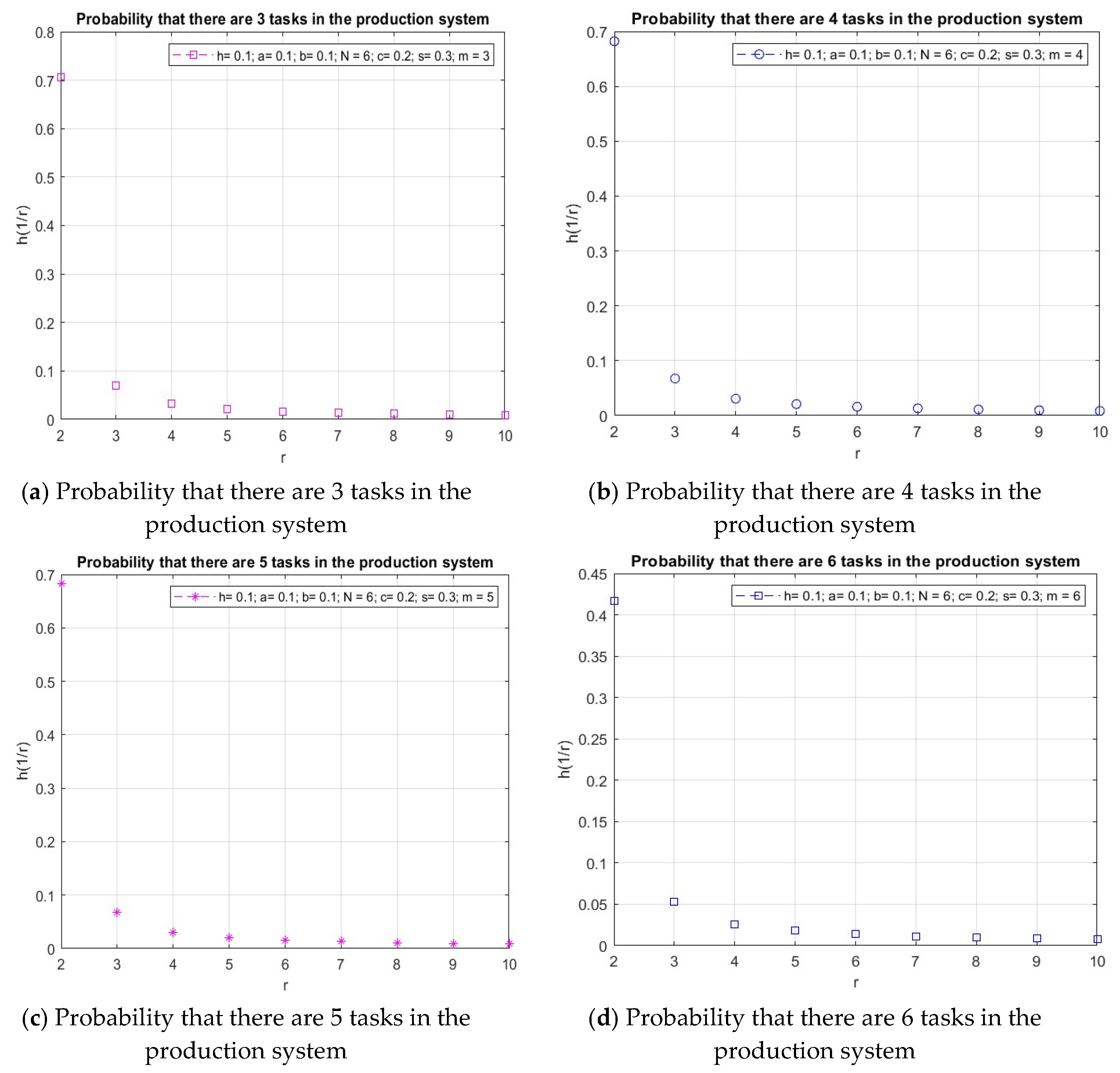
In the considered discrete-time queueing model with capacity N and with the mechanism of setup/close-down times, the queue-size distribution is conditioned by the initial accumulation buffer state. First is the maximal system capacity, $N=6$. Let $L_r$ denote the number of jobs present in the system exactly at time r, where $r=2,\dots ,10$, including a job whose service is in progress at time r, if any. Observe $L_6(r,3)$, the probability that at the fixed time $r=2,\dots ,10$ the number of jobs present in the system equals $m=3$ on the condition that initially (at time 0) the system (the input buffer, in fact) contains $i=6$ jobs,

$$\begin{array}{cc}\hfill & L_i(r,m)\stackrel{def}{=}\mathbf{P}\{L_r=3|L_0=6\},\hfill \end{array}$$

(55)

represented by Figure 2a. Similarly, $L_6(r,4)$, the probability that at the fixed time $r=2,\dots ,10$, the number of jobs present in the system equals $m=4$ on the condition that initially the system contains $i=6$ jobs, is presented in Figure 2b and $L_6(r,5)$, $L_6(r,6)$ in Figure 2c,d, respectively.

The probability that at the fixed time $r=2,\dots ,10$ the number of jobs present in the system equals $m=3,4,5,6$ decreases with time on the condition that initially the system contains $i=6$ jobs. The probability of more tasks present in a given time unit decreases as the number of analyzed tasks increases.

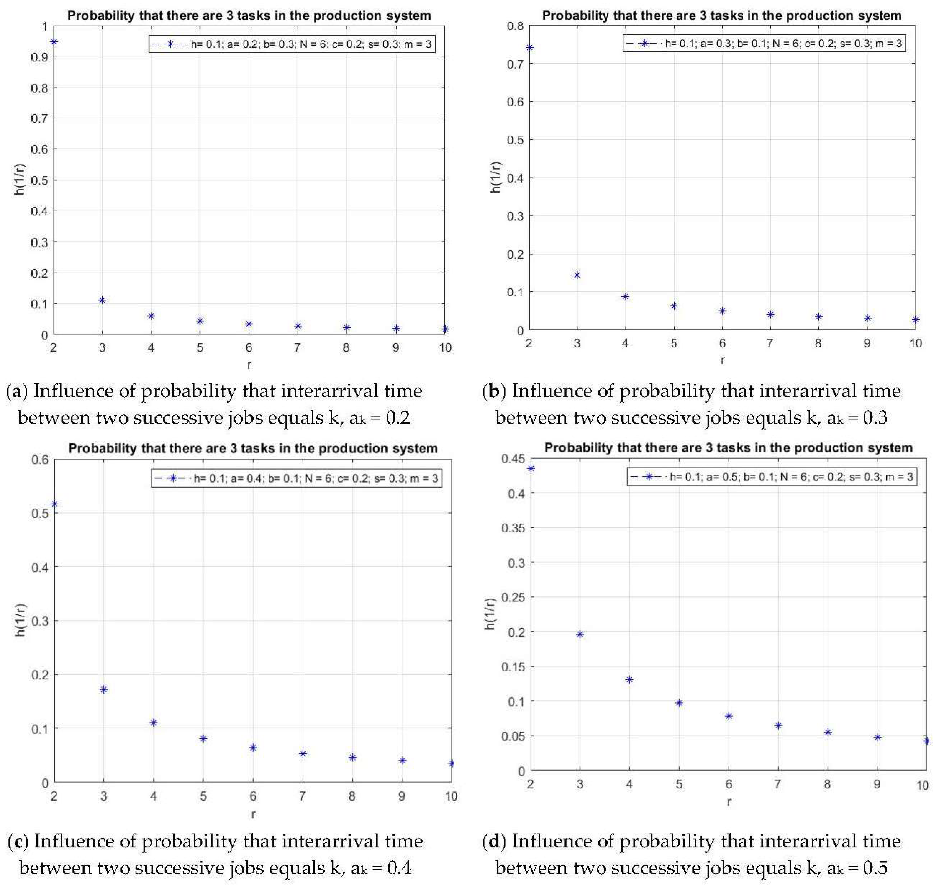
6.1. Impact of Probability That Interarrival Time between Two Successive Jobs Equals k Time Units

Observe $L_6(r,3)$, the probability that at the fixed time $r=2,\dots ,10$ the number of jobs present in the system equals $m=3$ on the condition that initially (at time 0) the system (the input buffer, in fact) contains $i=6$ jobs, $\{L_r=3|L_0=6\}$, and the probability that the interarrival time between two successive jobs equals k time units, $a_k=0.2$ (Figure 3a). The transient conditional distributions decrease after the production system is opened, starting from the peak obtained at time $r=2$.

Observe the influence of the probability that the interarrival time between two successive jobs equals k time units $a_k=0.2,0.3,0.4,0.5$ on the probability that at the fixed time $r=2,\dots ,10$ the number of jobs present in the system equals $m=3$ (Figure 3a–d). With the increase in $a_k$, the probability that at the moment $r=2,\dots ,10$ the number of jobs present in the system equals to $m=3$ decreases the most at the beginning of the production system operation. Starting from $r=6$, the effect of the probability that the interarrival time between two successive jobs equals to k time units $a_k=\{0.2,0.3,0.4,0.5\}$ becomes smaller and smaller. The longer the interarrival time between two successive jobs, the less impact there is on the production system described by $L_6(r,3)$.

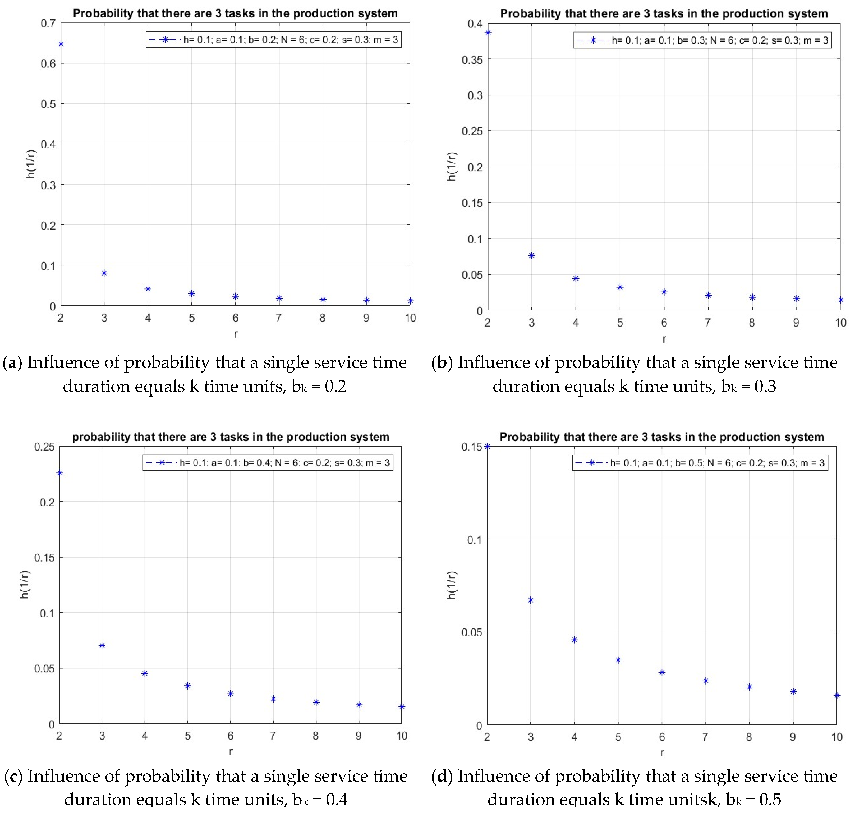
6.2. Impact of Probability That a Single Service Time Equals k Time Units

Observe $L_6(r,3)$, the probability that at the fixed time $r=2,\dots ,10$ the number of jobs present in the system equals $m=3$ on the condition that initially the input buffer contains $i=6$ jobs, $\{L_r=3|L_0=6\}$, and the probability that a single service time duration equals k time units $b_k=0.2$ (Figure 4a). The transient conditional distributions decrease most when the production system is opened, starting from the peak obtained at $r=2$. Given the probability that the duration of a single service is two time units, the probability that there are three jobs at this moment is $65\%$.

Observe the influence of the probability that a single service time equals k time units $b_k=0.2,0.3,0.4,0.5$ on the probability that at the fixed time $r=2,\dots ,10$ the number of jobs present in the system equals $m=3$ (Figure 4a–d). With the increase in $b_k$, the probability that at the moment $r=2,\dots ,10$ the number of jobs present in the system equals to $m=3$ decreases the most at the beginning of the production system operation. The effect of the probability that a single service time equals k time units $b_k=\{0.2,0.3,0.4,0.5\}$ becomes smaller and smaller. The longer a single service time of a job, the less impact there is on the production system described by $L_6(r,3)$.

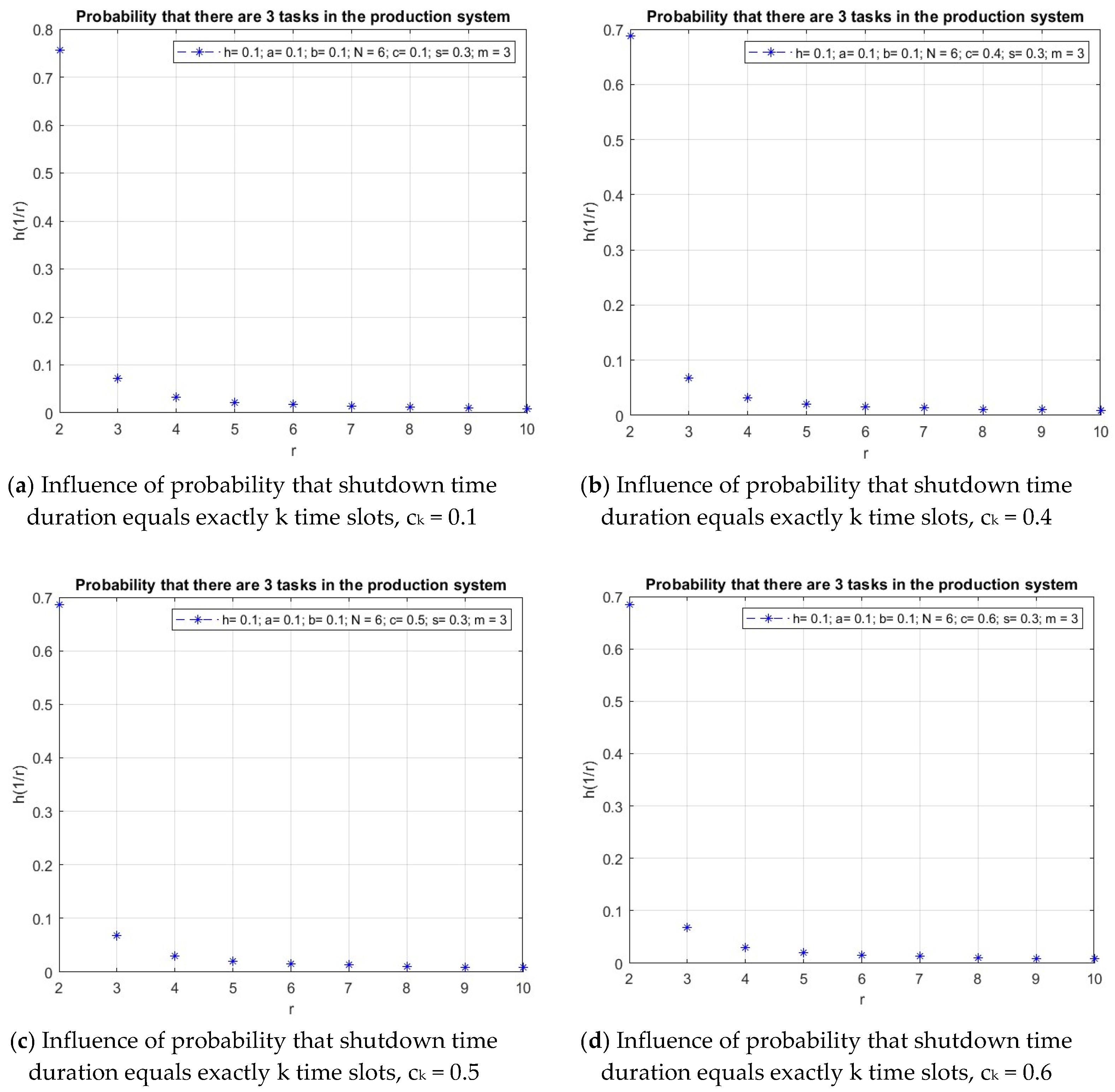
6.3. Impact of Probability That Shutdown Time Duration Equals Exactly k Time Slots

Observe $L_6(r,3)$, the probability that at the fixed time $r=2,\dots ,10$ the number of jobs present in the system equals $m=3$ on the condition $\{L_0=6\}$ and the probability that the shutdown time duration of the bottleneck equals k time units $c_k=0.1$ (Figure 5a). The transient conditional distributions decrease most when the production system is opened, starting from the peak obtained at $r=2$. Given the probability that the shutdown time duration of the bottleneck is two time units, the probability that there are three jobs at this moment is $76\%$.

Observe the influence of the probability that the shutdown time duration equals k time units $c_k=0,1,0.2,0.4,0.5$ on the probability that at the fixed time $r=2,\dots ,10$ the number of jobs present in the system equals $m=3$ (Figure 2a and Figure 5a–d). As $c_k$ increases, the probability that at the moment $r=2,\dots ,10$ the number of jobs present in the system equals to $m=3$ decreases the most at the beginning of the production system operation. The effect of the probability that the shutdown time duration equals k time units $c_k=\{0.1,0.2,0.4,0.5\}$ becomes lower and lower until the time $r=5$. The shutdown time duration of the bottleneck has no effect on the production system operation after $r=5$.

6.4. Impact of Probability That Setup Time Duration Equals Exactly k Time Slots

Observe $L_6(r,3)$, the probability that at the fixed time $r=2,\dots ,10$ the number of jobs present in the system equals $m=3$ on the condition $\{L_0=6\}$ and the probability that the setup time duration of the bottleneck equals k time units $s_k=0.2$ (Figure 6a). Again, the transient conditional distributions decrease most when the production system is opened. Given the probability that the setup time duration of the bottleneck is two time units, the probability that there are three jobs at this moment is $71\%$.

Observe the influence of the probability that the setup time duration equals k time units $c_k=0.2,0.3,0.4,0.5$ on the probability that at the fixed time $r=2,\dots ,10$ the number of jobs present in the system equals $m=3$ (Figure 2a and Figure 6a–d). As $s_k$ increases, the probability that at the moment $r=2,\dots ,10$ the number of jobs present in the system equals to $m=3$ decreases the most after opening the production system. The effect of the probability that the setup time duration equals k time units $s_k=\{0.2,0.3,0.4,0.5\}$ becomes lower and lower until the time $r=4$. Also, the setup time duration of the bottleneck has no effect on the production system operation after $r=5$.

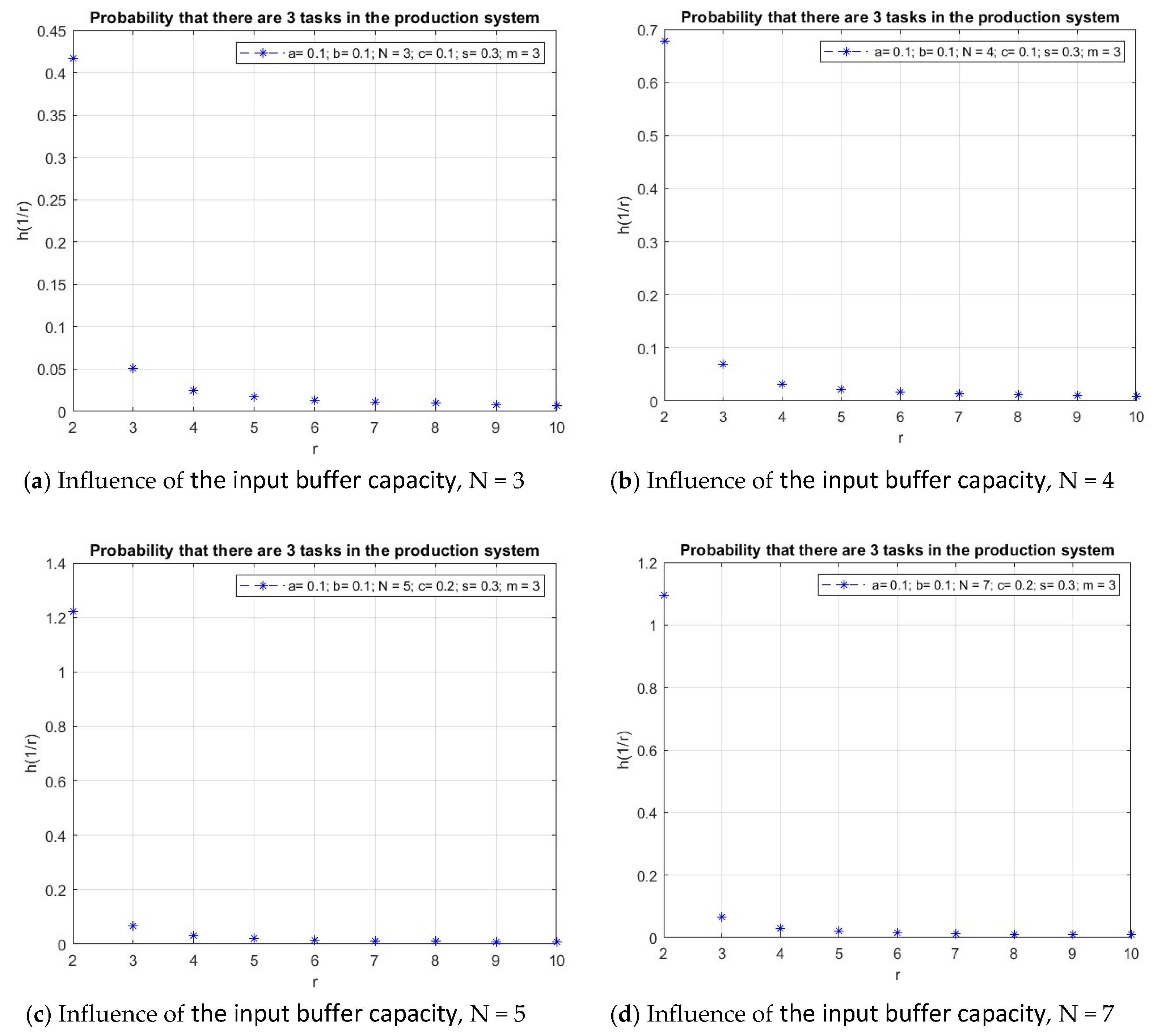
6.5. Impact of Input Buffer Size

Now observe the transient behavior of the considered probabilities, where the capacity of the production system $N=\{3,4,5,6,7\}$ (Figure 2a and Figure 7a–d). The probability that the interarrival time between two successive jobs equals k; the probability that a single service time duration equals k time slots; the probability that the shutdown time duration equals exactly k time slots; and the probability that the setup time duration is equal to k time units are described by the parameters $b=0.1,a=0.1,c=0.2$, and $s=0.3$ as in previous simulations.

In Figure 7a, the behavior of the system is considered for the maximal system capacity, $N=3$. The probabilities of three jobs $m=3$ in the system at time r (two jobs in the input buffer at the beginning, and one job in the bottleneck), provided that the input buffer contains $i=3$ jobs at time 1, decrease most when the production system is opened. After $r=5$, the production system is empty. The larger the input buffer capacity, the greater the probability of three jobs occurring in the production system (Figure 2a and Figure 7a–d).

6.6. Comparative Discussion on Energy-Saving Methods

To reduce production costs, researchers are optimizing batch sizes [43], minimizing losses [44], eliminating waste [45,46] and optimizing machine tools for efficient input and output [5]. Brundage [47] presents the possibility of saving energy based on a window calculated for on-line production data, which allows turning off a specific machine without negatively affecting throughput. Temporarily switching off a machine and switching it back on under a certain condition in order to save energy is also suggested by [48,49,50]. In our approach, we propose the switching-off strategy for the critical machine (if necessary) and extending the operating time of non-critical machines. Analyses are necessary to determine the most effective energy-reduction strategy: switching off a machine or slowing down its operation. The capacity and availability of a machine are reduced with the decision of switching off the machine because operations cannot be performed during setup or shutdown (warm up or cool down).

Continuous improvement and lean design for productivity and quality can lead to improved energy efficiency [45,46]. The common nature of our approach is the use of organizational improvement, i.e., the DBR concept, to reduce energy consumption. The minimum number of capacity buffers has a positive effect on the energy efficiency. By adjusting the interarrival time of orders and the input buffer size to the capacity of the bottleneck, the production system is well balanced, and the throughput of the production system is maximized. The opposite strategy is to add work-in-flow buffers between machines in a production system to maximize throughput and to protect machines from the consequences of failures and blocking [51,52]. According to the Theory of Constraints, the throughput of a production lines is equal to the capacity of the bottleneck. Therefore, the work-in-process buffer is necessary for the machine. However, the work-in-process buffer for the critical machine is actually just another machine that has a negative impact on the energy efficiency and costs of the production line. The analyzed literature ignores the impact of work-in-process buffers on the energy consumption. The advantage of methods for finding the best buffer allocation and optimizing both the throughput and energy consumption for serial production lines is the assumption that the machines are unreliable [51,52]. In particular, bottleneck downtime is crucial to the performance of production systems, upstream and downstream machine run times are shorter than cycle times, and work-in-process buffers may not be necessary. The maximum possible downtime of a non-critical machine without loss of production due to the i-th failure event is analyzed in [47]. The energy gain bottleneck is identified, i.e., the machine that causes the greatest loss of profit on the line. Downtime of the bottleneck and power bottleneck are analyzed to improve the energy efficiency and productivity of a production line in [53].

7. Conclusions

The aim of the paper was to analyze the impact of changes in key parameters of the production model controlled by DBR theory. The answer was sought to the question of how changing the values of key parameters dictated by the desire to reduce energy consumption affects the efficiency of the production system.

In the paper, a discrete-time queueing model of a production line with a single bottleneck and finite input buffer capacity was proposed. Jobs arrive according to a binomial process and are processed individually, one by one, according to the FIFO rule. Every time the system becomes empty, an energy-saving mechanism is started: the processing machine is turned off during a geometrically distributed shutdown time. The short interarrival time of jobs reduces the impact of the shutdown time of the bottleneck. The operation times of non-critical machines can be slowed down to reduce energy up to the takt time of the bottleneck.

The main analytic result of the article is a compact-form representation for the probability generating function of the transient queue-size distribution conditioned by the initial accumulation buffer state. To obtain this result, a theoretical approach based on using the total probability law, the method of generating functions, and linear algebra was applied. The appropriate stationary queue-size distribution is found from the main result directly by using the Abelian theorem.

The model of production system was built using Equations (20), (21), (25), (29), (30), (33)–(35), (39), (42), (45)–(48) and (51). Managers can study the behavior of a production system in terms of queue size by changing the key parameters of the input model (arrival intensity, bottleneck service rate, buffer size, and setup and shutdown times) to analyze the performance of the production system, including decisions regarding energy reduction. By adjusting the time between order arrivals and the size of the input buffer to the capacity of the bottleneck, the throughput of the production system is maximized. Also, the proposed strategy of shutting down the production line and slowing down the operation of non-critical machines balances the production system. One-piece flow with no work-in-process buffers reduces costs, saves energy and eliminate waste. In the paper, organizational and analytical solutions to model the sustainable production system are combined.

In the future, the model will be adopted to the theory of production control using Kanban cards. Possibilities of reducing energy consumption for the production system controlled by Kanban cards will be proposed. Moreover, the next planned steps to extend the considered model and obtain new results are the following:

• Modification of the energy-saving mechanism by adding a threshold discipline (N-policy), according to which the processing of jobs is restarted after an idle period if a fixed number of N jobs are accumulated in the buffer;
• Considering the case in which the arriving jobs occur in groups (batch arrival process), which, in general, can have random capacities;
• Investigating other stochastic and operational characteristic of the considered model, namely queueing delay (waiting time) distribution, time to buffer overflow and departure process.