


An Option Game Model of Supplier R&D Co-Competition under Uncertainty


Abstract
1. Introduction
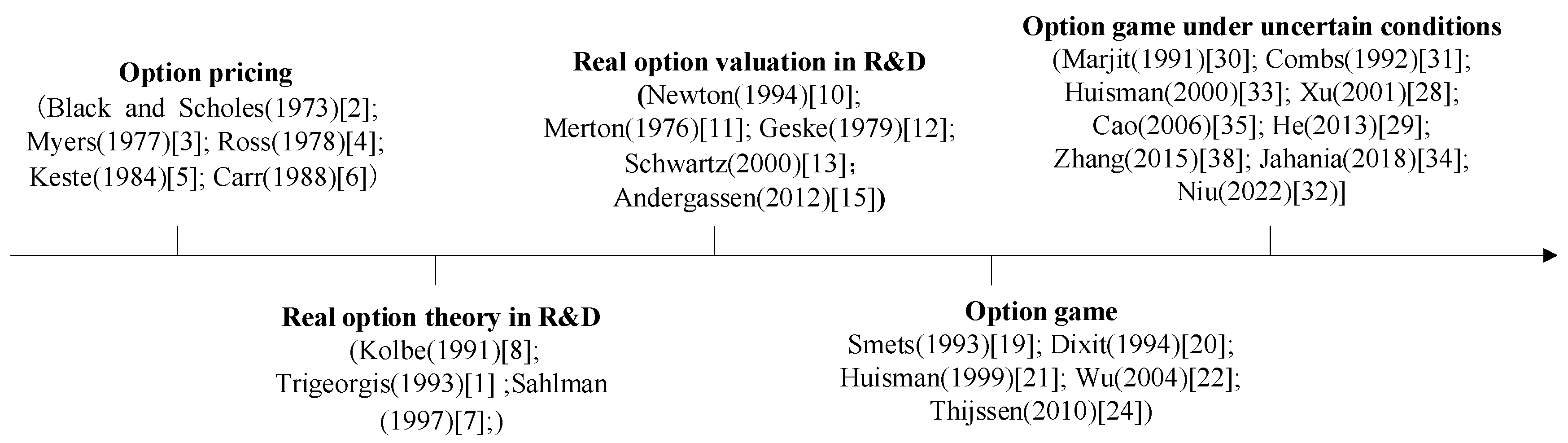
Literature Review
2. Construction of Investment Model
2.1. Model Assumptions
2.2. Investment Model
2.3. Enterprise Option Value
2.4. Investment Models under Different Investment Strategies
2.4.1. Waiting for Investment Strategy
2.4.2. Follow Investment Strategy
2.4.3. Leading Investment Strategy
2.4.4. Cooperative R&D Investment Strategy
3. Case Analysis
3.1. Case of Biolight
3.2. Investment Strategy Analysis
4. Sensitivity Analysis
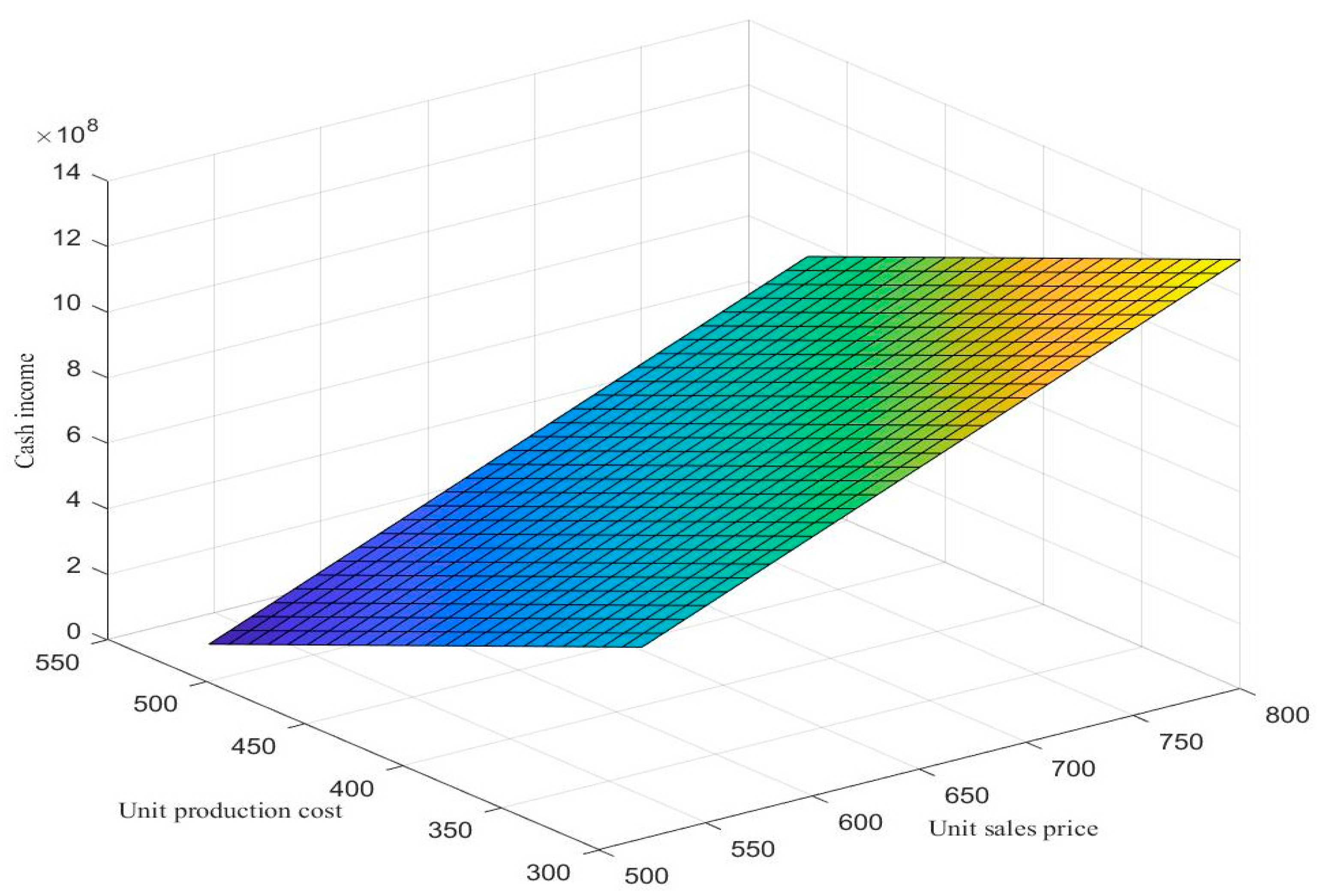
4.1. Impact of Changes in Selling Price and Cost on Expected Income
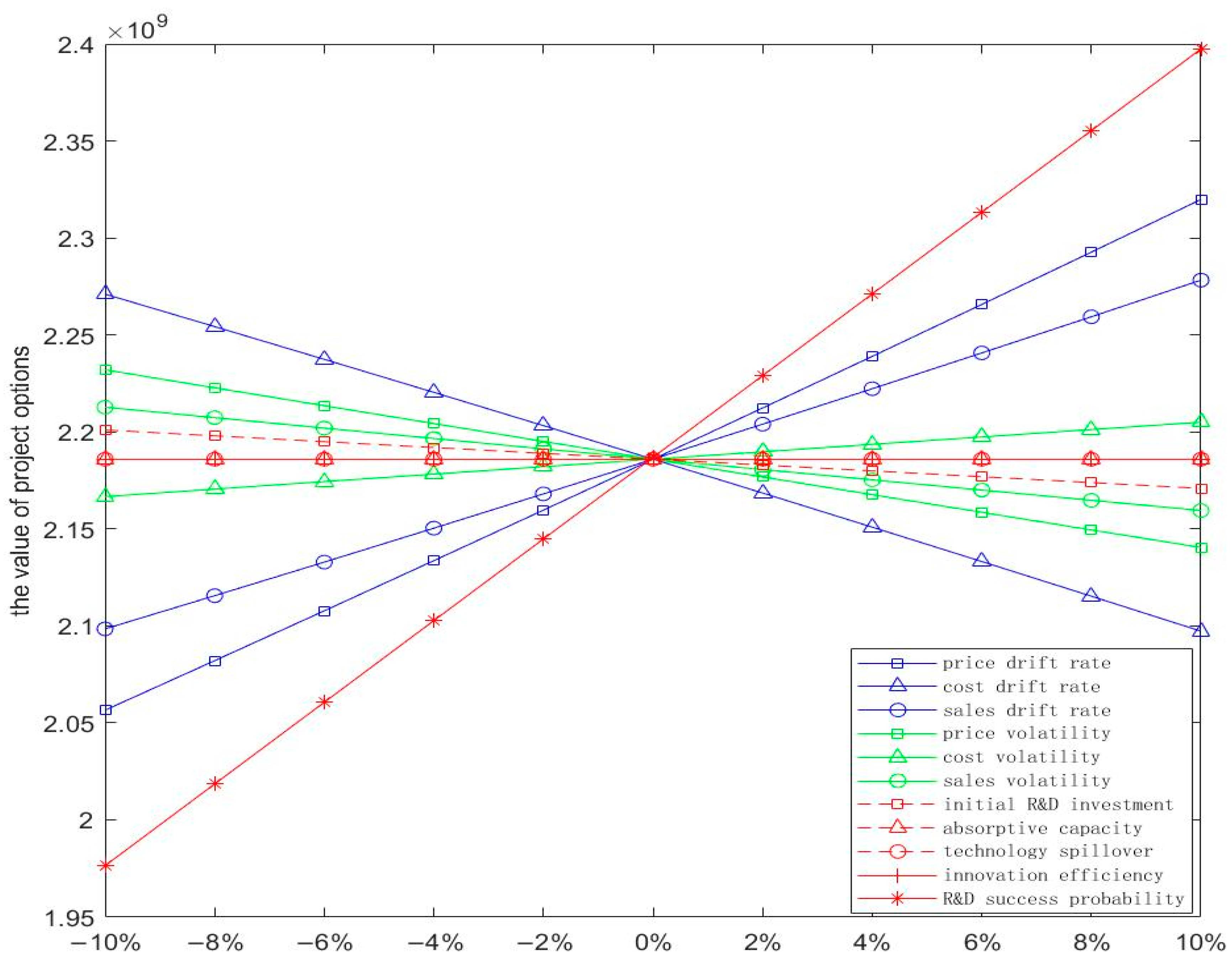
4.2. Impact of Changes in R&D Success Probability and One-Time R&D Investment on Project Option Value
5. Conclusions
Author Contributions
Funding
Institutional Review Board Statement
Data Availability Statement
Conflicts of Interest
References
- Baoting, W.; Hongwu, G. The Blue Book of Medical Device Industry: Annual Report on the Development Medical Device Industry in China (2021); Social Sciences Academic Press (CHINA): Beijing, China, 2021. [Google Scholar]
- Baoting, W.; Hongwu, G. The Blue Book of Medical Device Industry: Annual Report on the Development Medical Device Industry in China (2019); Social Sciences Academic Press (CHINA): Beijing, China, 2019. [Google Scholar]
- Trigeorgis, L. Real Options and Interaction with Financial Flexibility. Financ. Manag. 1993, 22, 202–224. [Google Scholar] [CrossRef]
- Black, F.; Scholes, M. The Pricing of Options and Corporate Liabilities. J. Polit. Econ. 1973, 81, 637–654. [Google Scholar] [CrossRef]
- Myers, S.C.; Turnbull, S.M. Capital Budgeting and the Capital Asset Pricing Model: Good News and Bad News. J. Financ. 1977, 32, 321–333. [Google Scholar] [CrossRef]
- Ross, S.A. A Simple Approach to the Valuation of Risky Streams. J. Bus. 1978, 51, 453–475. [Google Scholar] [CrossRef]
- Kester, W.C. Today’s Options for Tomorrow’s Growth. Harv. Bus. Rev. 1984, 62, 153–160. [Google Scholar] [CrossRef]
- Carr, P. The Valuation of Sequential Exchange Opportunities. J. Financ. 1988, 43, 1235–1256. [Google Scholar] [CrossRef]
- Shalman, W.A. How to Write a Great Business Plan. Harv. Bus. Rev. 1997, 75, 98–108. [Google Scholar]
- Morris, P.A.; Teisberg, E.O.; Kolbe, A.L. When Choosing R&D Projects, Go with Long Shots. Res. Technol. Manag. 1991, 34, 35–40. [Google Scholar] [CrossRef]
- Copeland, T.; Weiner, J. Proactive Management of Uncertainty. Mckinsey Q. 1990, 4, 133–152. [Google Scholar]
- Newton, D.P.; Pearson, A.W. Application of Option Pricing Theory to R&D. RD Manag. 1994, 24, 083–089. [Google Scholar] [CrossRef]
- Merton, R.C. Option Pricing When Underlying Stock Returns Are Discontinuous. J. Financ. Econ. 1976, 3, 125–144. [Google Scholar] [CrossRef]
- Geske, R. The Valuation of Compound Options. J. Financ. Econ. 1979, 7, 63–81. [Google Scholar] [CrossRef]
- Schwartz, E.S.; Moon, M. Rational Pricing of Internet Companies. Financ. Anal. J. 2000, 56, 62–75. [Google Scholar] [CrossRef]
- Schwartz, E.S. Patents and R&D As Real Options. Econ. Notes 2004, 33, 23–54. [Google Scholar] [CrossRef]
- Andergassen, R.; Sereno, L. Valuation of N-Stage Investments under Jump-Diffusion Processes. Comput. Econ. 2012, 39, 289–313. [Google Scholar] [CrossRef]
- Alvarez, L.H.R.; Stenbacka, R. Adoption of Uncertain Multi-Stage Technology Projects: A Real Options Approach. J. Math. Econ. 2001, 35, 71–97. [Google Scholar] [CrossRef]
- Lei, X.; Li, L. Research of R&D Investment under Competition Based on Option Games. J. Manag. S. 2004, 17, 85–89. [Google Scholar]
- Huang, X.; Wu, C. Option Game Model on R&D Investment Decision under Uncertainty. Chin. J. Manag. Sci. 2006, 14, 33–37. [Google Scholar] [CrossRef]
- Smets, F.R. Essays on Foreign Direct Investment. Ph.D. Thesis, Yale University, New Haven, CT, USA, 1993. [Google Scholar]
- Dixit, A.K.; Pindyck, S. Investment under Uncertainty; Princeton University Press: Princeton, NJ, USA, 1994. [Google Scholar]
- Huisman, K.J.M.; Kort, P.M. Effects of Strategic Interactions on the Option Value of Waiting; Working Paper; Tilburg University: Tilburg, The Netherlands, 1999. [Google Scholar]
- Wu, J.; Xuan, H. The Impact of Operating Costs on Firms’ R&D Investment Decision: A Real Option and Game-Theoretic Approach. Syst. Eng. 2004, 22, 30–34. [Google Scholar]
- Yang, Y.; Da, Q. Study on Investment in Technology Innovation of Asymmetric Duopoly. Chin. J. Manag. Sci. 2005, 13, 95–99. [Google Scholar] [CrossRef]
- Thijssen, J.J.J. Preemption in a Real Option Game with a First Mover Advantage and Player-Specific Uncertainty. J. Econ. Theory 2010, 145, 2448–2462. [Google Scholar] [CrossRef]
- Shibata, T. The Impacts of Uncertainties in a Real Options Model under Incomplete Information. Eur. J. Oper. Res. 2008, 187, 1368–1379. [Google Scholar] [CrossRef]
- Won, C. Valuation of Investments in Natural Resources Using Contingent-Claim Framework with Application to Bituminous Coal Developments in Korea. Energy 2009, 34, 1215–1224. [Google Scholar] [CrossRef]
- An, F.; Liu, G. Two-sided Beneficial Value-Added Service Investment and Pricing Strategies in Asymmetric/Symmetric Investment Scenarios. Symmetry 2023, 15, 1246. [Google Scholar] [CrossRef]
- Xu, M.; Zhang, Z. Application of Real Options Theory to R&D Project Evaluation. Syst. Eng. 2001, 19, 10–14. [Google Scholar]
- He, M.; Liu, J.; Gao, Q. An Investment Evaluation Model for Natural Resource Development Project under Multiple Uncertainties. J. Manag. Sci. China 2013, 16, 46–55. [Google Scholar]
- Marjit, S. Incentives for Cooperative and Non-Cooperative R and D in Duopoly. Econ. Lett. 1991, 37, 187–191. [Google Scholar] [CrossRef]
- Combs, K.L. Cost Sharing vs. Multiple Research Projects in Cooperative R&D. Econ. Lett. 1992, 39, 353–357. [Google Scholar] [CrossRef]
- Niu, W.; Shen, H. Investment in Process Innovation in Supply Chains with Knowledge Spillovers under Innovation Uncertainty. Eur. J. Oper. Res. 2022, 302, 1128–1141. [Google Scholar] [CrossRef]
- Huisman, K.J.M. Technology Investment: A Game Theoretic Real Options Approach; Springer: New York, NY, USA, 2001. [Google Scholar]
- Jahania, H.; Abbasia, B.; Alavifard, F.; Talluri, S. Supply Chain Network Redesign with Demand and Price Uncertainty. Int. J. Prod. Econ. 2018, 205, 287–312. [Google Scholar] [CrossRef]
- Cao, G.; Pan, Q. Investment Option-Game Equilibrium Strategy Analyses Based on Time-to-Build. Chinese. J. Manag. Sci. 2006, 14, 135–141. [Google Scholar] [CrossRef]
- Zhang, G.; Guo, J.; Liu, D. An Asymmetric Duopoly Option Game Model under Time-to-Build and Investment Cost. J. Manag. Sci. 2008, 21, 75–81. [Google Scholar] [CrossRef]
- Wang, X.; Zhang, S. Option Games in Finite Investment Project Life. Syst. Eng. Theory Pract. 2011, 31, 247–251. [Google Scholar] [CrossRef]
- Zhang, G.; Gao, X.; Wang, Y. An Asymmetric Duopoly Investment Decision-Making Model Based on Difference of Option. Syst. Eng. Theory Pract. 2015, 35, 751–762. [Google Scholar]
- Zheng, D.; Li, Z. Study on Compound Option Model Based on Asymmetric Volatilities. Syst. Eng. Theory Pract. 2003, 2, 14–18. [Google Scholar]
- Li, Z.W. Impact of Spillover Effects on Corporate R&D Behaviors. J. Xiamen Univ. (Arts Soc. Sci.) 2007, 3, 55–62. [Google Scholar]
- Nishihara, M. Valuation of R&D Investment under Technological, Market, and Rival Preemption Uncertainty. Manag. Decis. Econ. Int. J. Res. Prog. Manag. Econ. 2018, 39, 200–212. [Google Scholar] [CrossRef]
- Xie, B. Stackelberg Game R&D Investment Decision under Uncertainty of Demand and R&D Level. Sci. Technol. Manag. Res. 2021, 41, 7. [Google Scholar] [CrossRef]
- Li, W.; Liu, Y.; Chen, Y. Modeling a Two-Stage Supply Contract Problem in a Hybrid Uncertain Environment. Comput. Ind. Eng. 2018, 123, 289–302. [Google Scholar] [CrossRef]
- Song, Z.; He, S.; An, B. Decision and Coordination in a Dual-Channel Three-Layered Green Supply Chain. Symmetry 2018, 10, 549. [Google Scholar] [CrossRef]


| Date | Sales | Average Unit Cost (RMB) | Average Unit Selling Price (RMB) | Unit Profit (RMB) | Gross Profit Margin |
|---|---|---|---|---|---|
| 2015 | 137,248 | 718.24 | 1293.27 | 575.03 | 44.46% |
| 2016 | 228,567 | 495.41 | 958.42 | 463.02 | 48.31% |
| 2017 | 244,709 | 443.65 | 828.34 | 384.69 | 46.44% |
| 2018 | 250,249 | 503.62 | 937.17 | 433.55 | 46.26% |
| 2019 | 289,419 | 403.88 | 787.78 | 383.91 | 48.73% |
| 2020 | 817,093 | 439.25 | 948.24 | 508.99 | 53.68% |
| 2021 | 769,245 | 280.10 | 520.22 | 240.11 | 46.16% |
| Date | Sales | Average Unit Cost (RMB) | Average Unit Selling Price (RMB) | Unit Profit (RMB) | Gross Profit Margin |
|---|---|---|---|---|---|
| 2015 | 109,195 | 3753.17 | 11,994.13 | 8241 | 68.71% |
| 2016 | 124,644 | 3431.92 | 11,750.55 | 8319 | 70.79% |
| 2017 | 136,386 | 3251.07 | 11,878.97 | 8628 | 72.63% |
| 2018 | 171,869 | 3933.32 | 11,776.41 | 7843 | 66.60% |
Disclaimer/Publisher’s Note: The statements, opinions and data contained in all publications are solely those of the individual author(s) and contributor(s) and not of MDPI and/or the editor(s). MDPI and/or the editor(s) disclaim responsibility for any injury to people or property resulting from any ideas, methods, instructions or products referred to in the content. |
© 2023 by the authors. Licensee MDPI, Basel, Switzerland. This article is an open access article distributed under the terms and conditions of the Creative Commons Attribution (CC BY) license (https://creativecommons.org/licenses/by/4.0/).
Share and Cite
Song, Y.; Sang, X.; Wang, Z.; Xu, H. An Option Game Model of Supplier R&D Co-Competition under Uncertainty. Symmetry 2023, 15, 1584. https://doi.org/10.3390/sym15081584
Song Y, Sang X, Wang Z, Xu H. An Option Game Model of Supplier R&D Co-Competition under Uncertainty. Symmetry. 2023; 15(8):1584. https://doi.org/10.3390/sym15081584
Chicago/Turabian StyleSong, Yinghua, Xiaoyan Sang, Zhe Wang, and Hongqian Xu. 2023. "An Option Game Model of Supplier R&D Co-Competition under Uncertainty" Symmetry 15, no. 8: 1584. https://doi.org/10.3390/sym15081584
APA StyleSong, Y., Sang, X., Wang, Z., & Xu, H. (2023). An Option Game Model of Supplier R&D Co-Competition under Uncertainty. Symmetry, 15(8), 1584. https://doi.org/10.3390/sym15081584