Symmetry in a Fractional-Order Multi-Scroll Chaotic System Using the Extended Caputo Operator

Abstract

In this work, complex dynamics are found in a fractional-order multi-scroll chaotic system based on the extended Gamma function. Firstly, the extended left and right Caputo fractional differential operators are introduced. Then, the basic features of the extended left Caputo fractional differential operator are outlined. The proposed operator is shown to have a new fractional parameter (higher degree of freedom) that increases the system’s ability to display more varieties of complex dynamics than the corresponding case of the Caputo fractional differential operator. Numerical results are performed to show the effectiveness of the proposed fractional operators. Then, rich complex dynamics are obtained such as coexisting one-scroll chaotic attractors, coexisting two-scroll chaotic attractors, or approximate periodic cycles, which are shown to persist in a shorter range as compared with the corresponding states of the integer-order counterpart of the multi-scroll system. The bifurcation diagrams, basin sets of attractions, and Lyapunov spectra are used to confirm the existence of the various scenarios of complex dynamics in the proposed systems.

1. Introduction

In the current century, many engineers, scientists, and economists have described and analyzed their related problems using the aid of fractional calculus (FC) [1,2,3,4,5,6,7,8,9]. The primary rationale is that using FC provides a greater level of accuracy when measuring natural phenomena. Therefore, FC demonstrated immense potential for applications in various scientific and engineering fields. Notably, it has found utility in disciplines such as engineering [6], fluid dynamics [2], thermoelasticity [4,5], mathematical biology [1,8], as well as market dynamics [9]. Additionally, the biological models that are described in terms of FC involve the memory effect which is considered to be a powerful tool in modeling the epidemiological diseases and viral dynamics. In recent times, the Caputo fractional differential operator (CFDO) has gained significant importance as a valuable tool for modeling various scientific and engineering phenomena. This is primarily due to its ability to facilitate the determination of relevant initial values [10]. Consequently, the CFDO is widely used in real-world applications. Indeed, the CFDO is the classic left Caputo fractional differential operator (LCFDO).

On the other hand, chaotic attractors, present in both fractional- and integer-order equations, have demonstrated immense potential for applications in various technological and scientific fields. Notably, they have found utility in disciplines such as meteorological systems [11], chemical systems [12], as well as engineering systems [6,13,14,15]. The first chaotic attractor was discovered by Lorenz when he tried to make a mathematical model that can predict the weather [11]. Afterward, many chaotic attractors were reported by scientists such as Rossler system [12], Chua system [13], Chen system [14], Liu system [15], and MAVPD system [6]. Indeed, the Chua, Chen, Liu, and MAVPD systems are realized through an electronic circuit design. Recently, chaotic attractors in fractional-order equations were shown to have great potential applications in some technological and scientific disciplines such as the fractional Lorenz system [16], the fractional Chua system [17], the fractional Chen system [18], the fractional Rossler system [19], and the fractional MAVPD system [6]. In Ref. [7], the phase transition of chaotic attractors between the integer-order system and its fractional-order counterpart is discussed. It is found that under certain conditions, the chaotic attractors that appear in the fractional-order system may not exist in its integer-order counterpart. However, the periodic orbits that exist in the integer-order system cannot exist in its fractional-order counterpart involving the CFDO [20]. The approximate periodic cycles that may appear in the case of CFDO are due to the truncation error of the solution algorithm and the observation scale.

The multi-scroll chaotic system [21] is an autonomous dynamical system (DS) that has three quadratic nonlinearities. According to Ref. [22], this system is considered to be a transition system between the Chen system and the Lorenz system. So, the multi-scroll chaotic systems have promising applications to science and engineering.

One of the effective tools to describe the complex dynamics of the DS is the plot of the Poincaré points of a component of the solution for every period T of the external forcing signal against the system’s dynamical parameter. This tool is briefly termed the system’s bifurcation diagram. In such diagrams, the shaded (or colored) parts refer to regions where chaotic dynamics occur.

The Lyapunov exponents (LEs) are considered to be excellent estimators to quantify chaotic dynamics. The three-dimensional DS has a maximum of three LEs (${\mathsf{\Lambda }}_i,\hspace{0.17em}i=1,2,3$). In Ref. [23], Haken proved that one LE must vanish for any limit set other than an equilibrium point. Furthermore, one LE must vanish for continuous flows. When chaos exists, the system’s greatest LE must be positive. In addition, the third LE is negative for dissipative three-dimensional DS. Indeed, the sum of the LEs is the divergence of the flow corresponding to the DS. One of the most efficient numerical algorithms to estimate the LEs in the integer-order DS was reported by Wolf et al. [24]. In the fractional-order case, the LEs can successfully be estimated using the numerical algorithm given by Danca and Kuznetsov [25].

The extended Gamma function is a generalization of the well-known Euler Gamma function, which was discovered in the 18th century [26]. Recently, the extended Gamma function has had useful applications in science and engineering. Indeed, the LCFDO involves the Euler Gamma function. Hence, replacing the Euler Gamma function with the extended Gamma function in the Caputo fractional operators is an interesting line for research that was initiated by Matouk and Bachioua in Ref. [27]. Furthermore, in Ref. [28], Matouk and Bachioua investigated some chaotic behaviors in two fractional-order predator–prey models that consist of the generalized Caputo fractional operators. In Ref. [8], Matouk inserted the extended Gamma function into the CFDO for investigating the complex dynamics in an antimicrobial resistance model. These references [8,27,28] assert that the CFDO involving the extended Gamma function is more suitable to handle the complex dynamics arising from the models that describe the natural phenomena due to its high adequacy in predicting the models’ dynamics and also due to the existence of a higher degree of freedom that can be used to obtain more intricate dynamics that cannot present in the case of the corresponding classic fractional Caputo operators.

Here, we intend to investigate the chaotic dynamics of the multi-scroll chaotic system using the extended left Caputo fractional differential operators (ELCFDO). By introducing a new fractional parameter to the ELCFDO, more intricate dynamics can be achieved that were not present in the case of the corresponding classic LCFDO. This leads to the emergence of a diverse range of complex dynamics, including coexisting one-scroll chaotic attractors, coexisting two-scroll chaotic attractors, and approximate periodic cycles. Furthermore, advanced measures of DS such as bifurcation diagrams, basin sets of attractions (BSA), and Lyapunov spectra are utilized to validate the existence of these complex dynamics in multi-scroll chaotic systems. To summarize the main motivations in this article, we recall that the ELCFDO has a higher degree of freedom in comparison with the CFDO, which makes the multi-scroll chaotic system exhibit more scenarios of complex dynamics. In addition, the motivations of this work are clearly provided by comparing the results obtained via the ELCFDO with the results obtained via the classic integer- and fractional-order operators. Therefore, we compare the dynamics of the multi-scroll chaotic system involving the ELCFDO and the dynamics of the corresponding integer-order counterpart of the system by demonstrating the bifurcation diagrams and calculating the LEs. The outcome of this comparison asserts that the ELCFDO is a better candidate to handle the complex dynamics in the multi-scroll chaotic system since it provides varieties of complex dynamics that persist in a shorter range as compared with the corresponding states of the system’s integer-order counterpart.

The rest of this article is organized as follows. The basic definitions of the ELCFDO and the extended right Caputo fractional differential operators (ERCFDO) are introduced in Section 2. The integer-order multi-scroll chaotic system is introduced in Section 3, in which we provide the system’s bifurcation diagrams, the system’s Lyapunov spectra, and compute the system’s BSA. The fractional-order form of the multi-scroll chaotic system involving the ELCFDO is investigated in Section 4 where the system’s bifurcation diagrams and Lyapunov spectra are provided to confirm the main motivations of this work. Finally, we provided the concluding statements and future studies in Section 5.

Notations: Throughout this article, the sets of positive (negative) real numbers are, respectively, represented by $R^{+}(R^{-}).$ The set of all natural numbers is represented by $N.$ $AC([u,v])$ represents the set of all functions that are absolutely continuous on the interval $[u,v]$. The expression of the ceiling function is represented by $⌈.⌉.$

2. Fractional Calculus

The ELCFDO is described by

$${}_C{}^E{\rm O}_{u+}^{q,\eta }\kappa (t)={{\rm K}}_{u+}^{l-q,\eta }\frac{d^l\kappa (t)}{d{t}^l},\hspace{0.17em}\hspace{0.17em}\hspace{0.17em}q\in R^{+},$$

(1)

where $l=⌈q⌉$, ${{\rm K}}_{u+}^{\xi ,\eta }\phi (t)=[{\displaystyle \underset{u}{\overset{t}{\int }}\frac{\phi (x)}{{(t-x)}^{1-\xi }}}dx]/{\Gamma }_0(\xi ,\eta ),\hspace{0.17em}\hspace{0.17em}\hspace{0.17em}\xi \in R^{+},\hspace{0.17em}\hspace{0.17em}t>u,$ represents the $\xi$th-order extended left Riemann–Liouville (ELRL) fractional integral, where ${\Gamma }_0(\xi ,\eta )$ is the extended Gamma function defined by

$${\Gamma }_0(\xi ,\eta )=\left[{\displaystyle \underset{0}{\overset{+\infty }{\int }}\frac{y^{\xi -1}}{e^y}}dy\right]/{\eta }^{\xi },\hspace{0.17em}\hspace{0.17em}\hspace{0.17em}\xi ,\hspace{0.17em}\eta \in R^{+}.$$

(2)

However, the $\xi$th-order extended right Riemann–Liouville (ERRL) fractional integral is

$${{\rm K}}_{v-}^{\xi ,\eta }\phi (t)=[{\displaystyle \underset{t}{\overset{v}{\int }}\frac{\phi (x)}{{(x-t)}^{1-\xi }}}dx]/{\Gamma }_0(\xi ,\eta ),\hspace{0.17em}\hspace{0.17em}\hspace{0.17em}\xi \in R^{+},\hspace{0.17em}\hspace{0.17em}t<v.$$

(3)

Hence, the ERCFDO is given by

$${}_C{}^E{\rm O}_{v-}^{q,\eta }\kappa (t)={{\rm K}}_{b-}^{l-q,\eta }{(-\frac{d}{dt})}^l\kappa (t),\hspace{0.17em}\hspace{0.17em}\hspace{0.17em}q\in R^{+},\hspace{0.17em}\hspace{0.17em}l\in N.$$

(4)

The following relations hold for the ELCFDO

(i)

Let $c\in R\backslash \left\{0\right\}$ be a constant number then ${}_C{}^E{\rm O}_{u+}^{q,\eta }c=0$.

(ii)

Let $\kappa (t)\in AC([u,v])$ and $q\in (0,1]$, then

$$\underset{q\to 1}{\lim }{}_C{}^E{\rm O}_{u+}^{q,\eta }\kappa (t)=\frac{d\kappa (t)}{dt}.$$

(5)

Furthermore, the following properties for the ELRL fractional integral hold

$$\begin{array}{ll}(I)& {{\rm K}}_{u+}^{1,\eta }\kappa (t)=\eta {\displaystyle \underset{u}{\overset{t}{\int }}\kappa (x)dx}.\\ (II)& \mathrm{If} \kappa (t)\in L^1, \mathrm{then} {{\rm K}}_{u+}^{{\xi }_1,\eta }\hspace{0.17em}\hspace{0.17em}{{\rm K}}_{u+}^{{\xi }_2,\eta }\kappa (t)={{\rm K}}_{u+}^{{\xi }_1+{\xi }_2,\eta }\kappa (t).\\ (III)& \underset{\xi \to l}{\lim }{{\rm K}}_{u+}^{\xi ,\eta }\kappa (t)={{\rm K}}_{u+}^{l,\eta }\kappa (t) \mathrm{uniformly} \mathrm{on} [u,v],\hspace{0.17em}\hspace{0.17em}l=1,\hspace{0.17em}2,\hspace{0.17em}3,\dots .\\ (IV)& \underset{\xi \to 0}{\lim }{{\rm K}}_{u+}^{\xi ,\eta }\kappa (t)=\kappa (t) \mathrm{weakly}.\\ (V)& \mathrm{If} 0<\xi <1 \mathrm{and} \kappa \in C[0,v] \mathrm{then} {\left.{{\rm K}}_{0+}^{\xi ,\eta }\kappa (t)\right|}_{t=0}=0.\\ (VI)& {{\rm K}}_{u+}^{{\xi }_1,\eta }\hspace{0.17em}\hspace{0.17em}{{\rm K}}_{u+}^{{\xi }_2,\eta }\kappa (t)={{\rm K}}_{u+}^{{\xi }_2,\eta }\hspace{0.17em}\hspace{0.17em}{{\rm K}}_{u+}^{{\xi }_1,\eta }\kappa (t) \forall {\xi }_1,\hspace{0.17em}\hspace{0.17em}{\xi }_2\in R^{+}\cup \left\{0\right\}.\\ (VII)& {{\rm K}}_{0+}^{\xi ,\eta }{t}^n=\frac{{\Gamma }_0(1+n,\eta )}{{\Gamma }_0(1+n+\xi ,\eta )}{t}^{\xi +n} \forall n>-1.\end{array}$$

(6)

The relation between the ELCFDO and the classic CFDO (${}_C{}^{}{\rm O}_{u+}^q\kappa (t)$) is given as

$${}_C{}^E{\rm O}_{u+}^{q,\eta }\kappa (t)={\eta }^{l-q}\hspace{0.17em}{}_C{}^{}{\rm O}_{u+}^q\kappa (t),\hspace{0.17em}\hspace{0.17em}\hspace{0.17em}\eta ,q\in R^{+},$$

(7)

where $l=⌈q⌉.$ The parameter $\eta$ acts as a higher degree of freedom for the ELCFDO. Hence, more intricate dynamics can be achieved that were not present in the case of the corresponding classic LCFDO. This leads to the emergence of a diverse range of complex dynamics.

3. Description of the Integer-Order Multi-Scroll Chaotic System

The classic multi-scroll chaotic system [21] is presented as

$$\begin{array}{l}\frac{d{\beta }_1}{dt}=c-d{\beta }_1-{\beta }_2{\beta }_3,\\ \frac{d{\beta }_2}{dt}=a{\beta }_2+{\beta }_1{\beta }_3,\hspace{0.17em}\hspace{0.17em}\hspace{0.17em}\hspace{0.17em}\\ \frac{d{\beta }_3}{dt}\hspace{0.17em}=b{\beta }_3+{\beta }_1{\beta }_2,\end{array}$$

(8)

where $d=\frac{ab}{b+a}$.

Obviously, the divergence of the system (8) is given as div(F) = a + b − d, where F represents the flow vector. Hence, the integer-order multi-scroll system (8) is dissipative if and only if the quantity div(F) is negative. This means that the volume element $V_0$ converges to zero as the time t increases to infinity at an exponential rate, a + b − d. Therefore, the motion of all the system orbits asymptotically settles onto an attractor. In addition, the integer-order multi-scroll chaotic system (8) has a highly symmetric structure that makes the system robust to different small perturbations. Thus, chaotic attractors are expected in this system when it undergoes sensitive dependence on initial data. One-scroll and two-scroll chaotic attractors in this system are obtained using the parameter sets $A=\{a,\hspace{0.17em}b,\hspace{0.17em}c\}=\{-10,-4,18.1\}$ and $B=\{a,\hspace{0.17em}b,\hspace{0.17em}c\}=\{-10,-4,0\},$ respectively. For, $a,b\in R^{-}$ and $c>-\frac{{\gamma }^{\frac{3}{2}}}{b+a},\hspace{0.17em}\hspace{0.17em}\gamma =\sqrt{ab},$ the system’s equilibrium points are

$${{\rm P}}_1=(\frac{c}{d},0,0),{{\rm P}}_{2,3}=(\gamma ,\pm \frac{\gamma }{a}\sqrt{\frac{d{\gamma }^2-\gamma c}{b}},\pm \sqrt{\frac{d{\gamma }^2-\gamma c}{b}}),{{\rm P}}_{4,5}=(-\gamma ,\pm \frac{\gamma }{a}\sqrt{\frac{d{\gamma }^2-\gamma c}{b}},\pm \sqrt{\frac{d{\gamma }^2-\gamma c}{b}}).$$

(9)

The above-mentioned equilibria are reduced to only three when using selection A of the parameter values. So, we obtain

$${{\rm P}}_1=(\frac{c}{d},0,0) \mathrm{and} {{\rm P}}_{2,3}=(\gamma ,\pm \frac{\gamma }{a}\sqrt{\frac{d{\gamma }^2-\gamma c}{b}},\pm \sqrt{\frac{d{\gamma }^2-\gamma c}{b}}).$$

(10)

For $a,b\in R^{-}$ and $c=0,$ the system’s equilibrium points are

$${{\rm P}}_0=(0,0,0),{{\rm P}}_{2,3}=(\gamma ,\pm \frac{\gamma }{a}\sqrt{\frac{a{\gamma }^2}{b+a}},\pm \sqrt{\frac{a{\gamma }^2}{b+a}}),{{\rm P}}_{4,5}=(-\gamma ,\pm \frac{\gamma }{a}\sqrt{\frac{a{\gamma }^2}{b+a}},\pm \sqrt{\frac{a{\gamma }^2}{b+a}}).$$

(11)

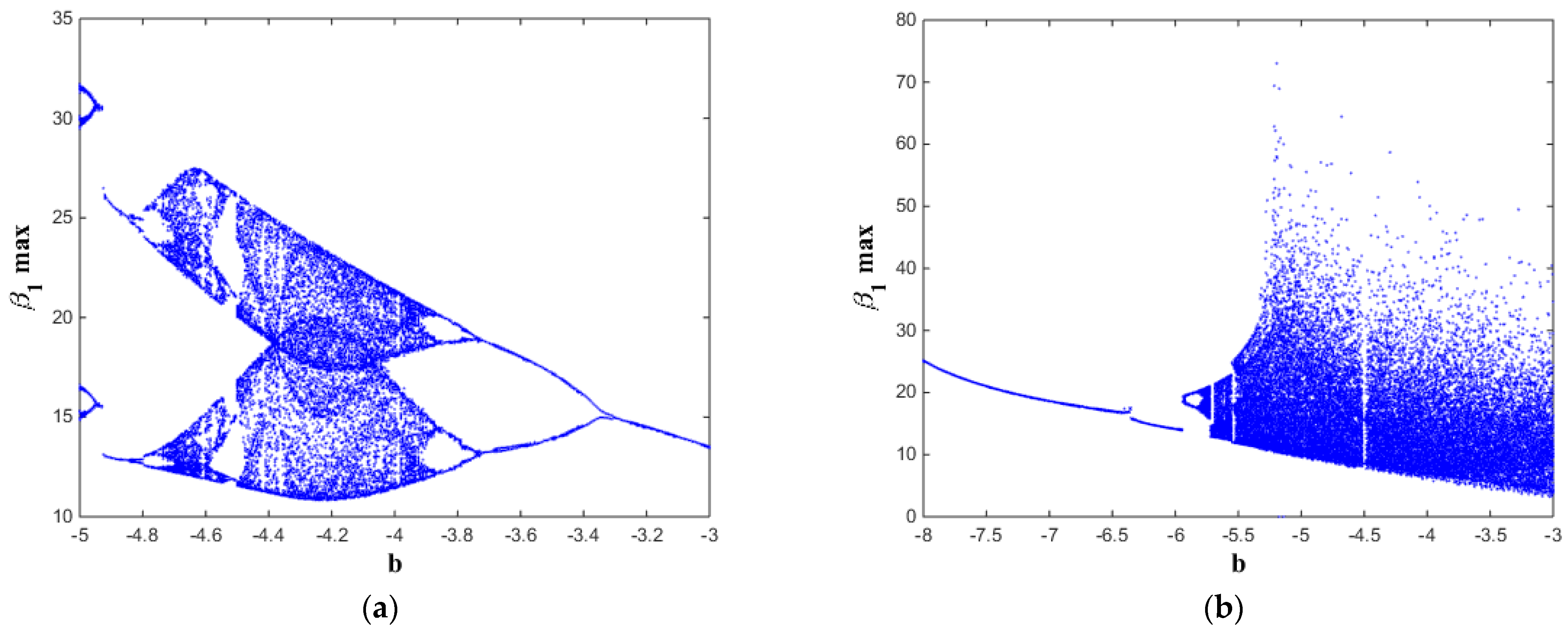
System (8) is numerically integrated based on the MATLAB command ODE45 to obtain its bifurcation diagrams (See Figure 1, Figure 2 and Figure 3) and the BSA. The initial states are chosen as $({\beta }_{10},{\beta }_{20},{\beta }_{30})=(0.1,0.1,0.1)$. The bifurcation diagrams confirm the existence of a rich variety of chaotic attractors in this system and different routes to chaos via period-doubling bifurcations.

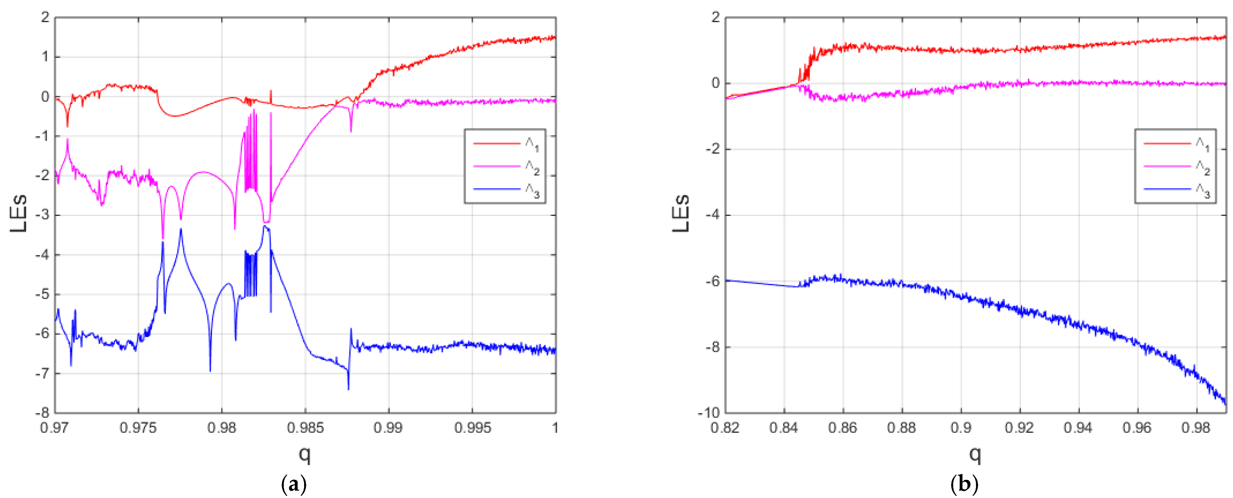
The corresponding Les are calculated based on the numerical algorithm in Ref. [24]. Furthermore, the Lyapunov spectra of the system (8) are also obtained to confirm the existence of such wide regions of chaotic dynamics. The results are depicted in Figure 4, Figure 5 and Figure 6.

The bifurcation diagrams and the Les illustrate the region of chaotic dynamics in the system (8) as follows. In Figure 1, chaotic dynamics exist when −11 < a ≤ −8.96 (see Figure 1a) and exist when −11 ≤ a ≤ −7 (See Figure 1b). In Figure 2, chaotic dynamics exist when −4.7 < b ≤ −4 (see Figure 2a) and exist when −5.7 < b ≤ −3 (see Figure 2b). In Figure 3, chaotic dynamics exist when 17 < c < 19.3 (see Figure 3a) and exist when 0 ≤ c < 12 and 15 ≤ c ≤ 19 (see Figure 3b).

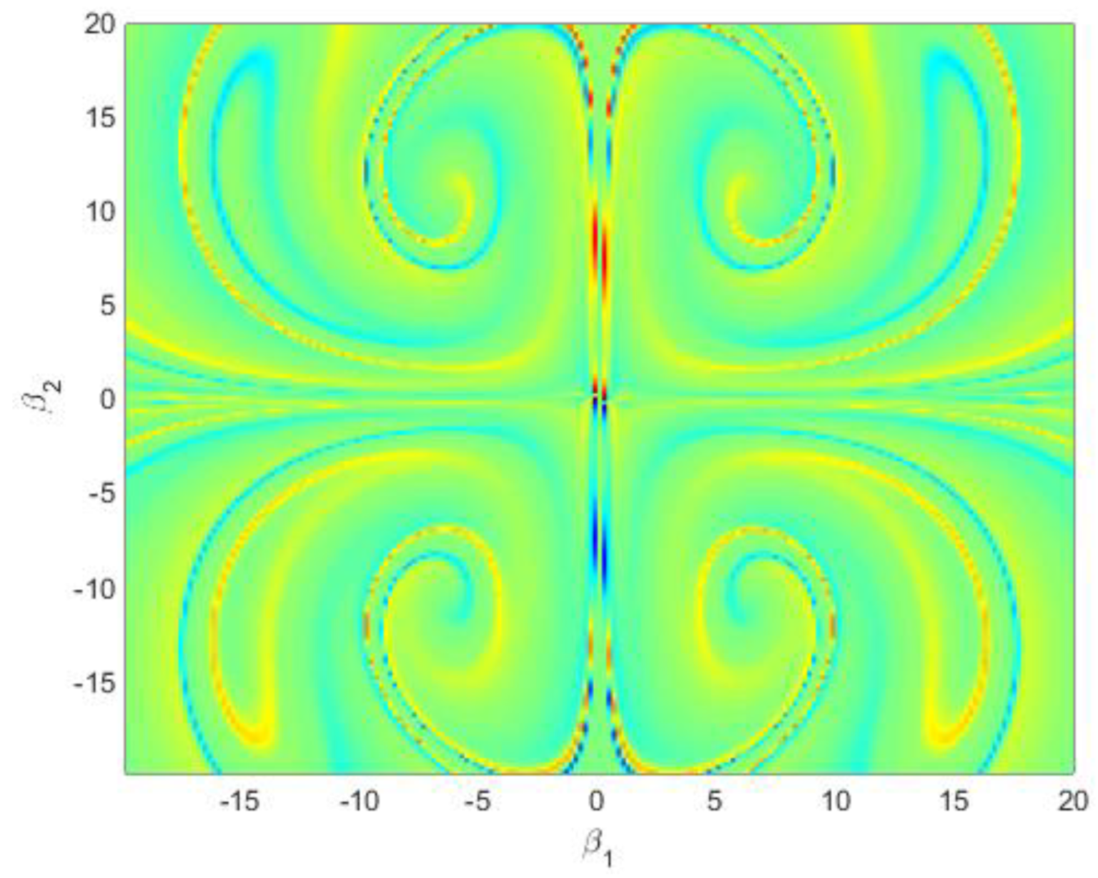
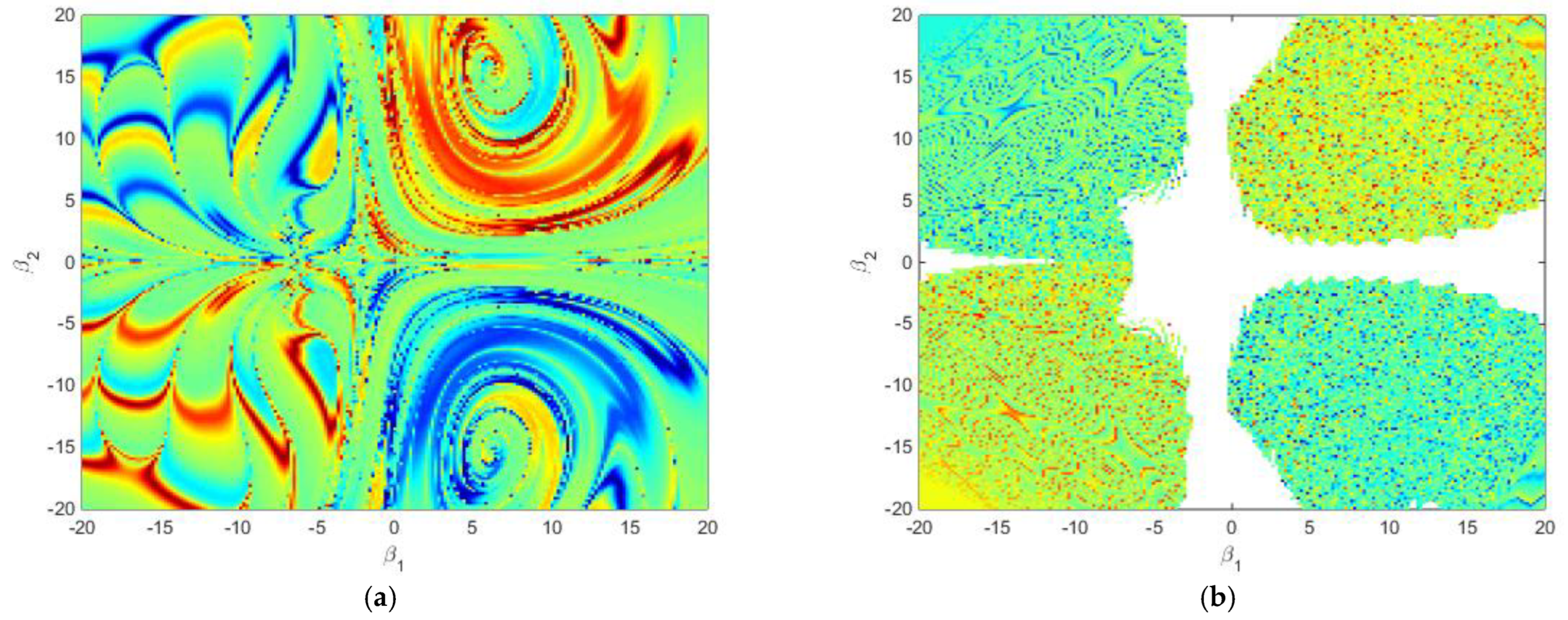
The BSA is given in the Figure 4 and Figure 5 to confirm the coexistence of multi-attractors in this system. In Figure 7, the blue and the red regions refer to the coexisting two one-band chaotic attractors. In Figure 8, the yellow and the turquoise regions refer to the coexisting two double-band chaotic attractors.

4. The Fractional-Order Multi-Scroll Chaotic System via the ELCFDO

The fractional-order version of the system (8) via the ELCFDO is given by

$$\begin{array}{l}{}_C{}^E{\rm O}_{0+}^{q,\eta }{\beta }_1=c-d{\beta }_1-{\beta }_2{\beta }_3,\\ {}_C{}^E{\rm O}_{0+}^{q,\eta }{\beta }_2=a{\beta }_2+{\beta }_1{\beta }_3,\hspace{0.17em}\hspace{0.17em}\hspace{0.17em}\hspace{0.17em}\hspace{1em}q\in (0,1).\\ \hspace{0.17em}{}_C{}^E{\rm O}_{0+}^{q,\eta }{\beta }_3=b{\beta }_3+{\beta }_1{\beta }_2,\end{array}$$

(12)

Since the ELCFDO is a linear operator, we obtain ${}_C{}^E{\rm O}_{0+}^{q,\eta }(-{\beta }_i(t))=-{}_C{}^E{\rm O}_{0+}^{q,\eta }({\beta }_i(t)),\hspace{0.17em}\hspace{0.17em}i=1,2,3$ . So, the multi-scroll chaotic system (12) is symmetrical about the ${\beta }_i-axis,\hspace{0.17em}\hspace{0.17em}i=1,2,3$ due to the invariance of this system under the transforms $({\beta }_1,{\beta }_2,{\beta }_3)\to ({\beta }_1,-{\beta }_2,-{\beta }_3),\hspace{0.17em}\hspace{0.17em}({\beta }_1,{\beta }_2,{\beta }_3)\to (-{\beta }_1,{\beta }_2,-{\beta }_3),$ and $({\beta }_1,{\beta }_2,{\beta }_3)\to (-{\beta }_1,-{\beta }_2,{\beta }_3)$.

Then, numerical simulations based on the modified PECE scheme [27] are carried out for the system (12) using the parameter sets A and B. Throughout the simulations, the selection of initial values $({\beta }_{10},{\beta }_{20},{\beta }_{30})=(0.1,0.1,0.1)$ and $({\beta }_{10},{\beta }_{20},{\beta }_{30})=(0.1,0.1,-0.1)$ are used for the upper attractors (red domain) and the lower attractors (blue domain), respectively. In Figure 9, coexisting upper and lower one-scroll chaotic attractors and approximate periodic cycles are shown. In Figure 10, different types of coexisting upper and lower two-scroll chaotic attractors with different intensities are depicted.

The bifurcation diagrams for system (12) are obtained via the local maxima algorithm to confirm the existence of a wide range of chaotic dynamics. The results are depicted in Figure 11, Figure 12, Figure 13 and Figure 14.

On the other hand, the Les are calculated based on the numerical algorithm in Ref. [25]. Furthermore, the Lyapunov spectra of the system (12) are also obtained to confirm the existence of such wide regions of chaotic dynamics. Then, the results are depicted in Figure 15, Figure 16, Figure 17 and Figure 18.

The region of chaotic dynamics in the system (12) can be illustrated via the bifurcation diagrams and the Les as follows. In Figure 11, chaotic dynamics exist when −11 < a ≤ −8.9 (see Figure 11a) and exist when −11 ≤ a ≤ −7 (see Figure 11b). In Figure 12, chaotic dynamics exist when −5 ≤ b < −4 (see Figure 12a) and exist when −6.5 < b < −5.7, and −5.7 < b < −4.1 (see Figure 12b). In Figure 13, chaotic dynamics exist when 17 < c ≤ 17.2, and 17.3 < c ≤ 18 (see Figure 13a) and exist when 0 ≤ c < 13, and 13 < c ≤ 17 (see Figure 13b). In most corresponding cases, except Figure 2a and Figure 12a observe that the chaotic dynamics in the multi-scroll chaotic system involving the ELCFDO are displayed in shorter ranges when compared with the system’s integer-order form. Furthermore, the approximate periodic cycles in Figure 12a exist in a shorter range than the corresponding periodic orbits in Figure 2a. Thus, the ELCFDO can be implemented to shorten the complex dynamics in this system using a suitable choice of the new fractional parameter η.

Figure 19 is carried out to confirm the existence of a higher degree of unpredictability and complexity of basins’ structures in the system (12). In Figure 19a, the blue and the red regions refer to the coexisting two approximate period 4 cycles. In Figure 19b, the coexisting two approximate higher periodic cycles are characterized by the dotted line and the dotted turquoise regions.

5. Conclusions

The ERCFDO and ELCFDO have been presented, and some related mathematical relations have been provided. Complex dynamics have been found in the fractional multi-scroll chaotic system using the ELCFDO. It has been found that the new parameter of the ELCFDO helps the multi-scroll chaotic system to exhibit more complex dynamics that cannot be found in its counterpart with the classic LCFDO. As an illustration, a wide array of complex dynamics are achieved, encompassing coexisting one-scroll chaotic attractors, coexisting two-scroll chaotic attractors, and approximate periodic cycles. Furthermore, advanced measures of DS such as the bifurcation diagrams, basin sets of attraction, and Lyapunov spectra have been utilized to confirm the existence of the complex dynamics in the multi-scroll chaotic systems.

Throughout this article, some comparisons have been performed by demonstrating the systems’ bifurcation diagrams and calculating the systems’ LEs, which illustrate that full scenarios of complex dynamics in the multi-scroll chaotic system involving the ELCFDO persist in a shorter range as compared with the corresponding states of the system’s integer-order counterpart. Moreover, the higher degree of freedom in the case of the ELCFDO increases the system’s ability to display more varieties of complex dynamics than the corresponding CFDO case. The summary of such results indicates that the ELCFDO is a better choice to describe the complex dynamics of the multi-scroll chaotic system.

Future studies can be extended to implement microcontroller-based circuits based on the multi-scroll chaotic system involving the ELCFDO, which may be useful in real digital engineering applications such as secure communication. Studying chaos control and synchronization in the multi-scroll chaotic system involving the ELCFDO are also two main points of interest for future works.

References

1. Ahmed, E.; Elgazzar, A.S. On fractional order differential equations model for non-local epidemics. Phys. A 2007, 379, 607–614. [Google Scholar] [CrossRef] [PubMed]
2. Abbas, S.; Nazar, M.; Nisa, Z.U.; Amjad, M.; El Din, S.M.; Alanzi, A.M. Heat and Mass Transfer Analysis of MHD Jeffrey Fluid over a Vertical Plate with CPC Fractional Derivative. Symmetry 2022, 14, 2491. [Google Scholar] [CrossRef]
3. Kumar, A.; Alzaid, S.S.; Alkahtani, B.S.T.; Kumar, S. Complex Dynamic Behaviour of Food Web Model with Generalized Fractional Operator. Mathematics 2022, 10, 1702. [Google Scholar] [CrossRef]
4. Zenkour, A.; Abouelregal, A. Fractional thermoelasticity model of a 2D problem of mode-I crack in a fibre-reinforced thermal environment. J. Appl. Comput. Mech. 2019, 5, 269–280. [Google Scholar] [CrossRef]
5. Abouelregal, A.; Ahmad, H. A Modified Thermoelastic Fractional Heat Conduction Model with A Single-Lag and Two Different Fractional-Orders. J. Appl. Comput. Mech. 2021, 7, 1676–1686. [Google Scholar] [CrossRef]
6. Matignon, D. Stability results for fractional differential equations with applications to control processing. In Proceedings of the Computational Engineering in Systems and Application Multi-Conference, IMACS, IEEE-SMC Proceedings, Lille, France, 9–12 July 1996; Volume 1, pp. 963–968. [Google Scholar]
7. Matouk, A.E. Chaotic attractors that exist only in fractional-order case. J. Adv. Res. 2023, 45, 183–192. [Google Scholar] [CrossRef]
8. Matouk, A.E. Applications of the generalized gamma function to a fractional-order biological system. Heliyon 2023, 9, e18645. [Google Scholar] [CrossRef]
9. Laskin, N. Fractional market dynamics. Phys. A 2000, 287, 482–492. [Google Scholar] [CrossRef]
10. Caputo, M. Linear Models of Dissipation whose Q is almost Frequency Independent—II. Geophys. J. R. Astron. Soc. 1967, 13, 529–539. [Google Scholar] [CrossRef]
11. Lorenz, E.N. Deterministic nonperiodic flow. J. Atmos. Sci. 1963, 20, 130–141. [Google Scholar] [CrossRef]
12. Rössler, O.E. An equation for continuous chaos. Phys. Rev. A 1976, 57, 397–398. [Google Scholar] [CrossRef]
13. Chua, L.O.; Lin, G.-N. Canonical realization of Chua's circuit family. IEEE Trans. Circuits Syst. 1990, 37, 885–902. [Google Scholar] [CrossRef]
14. Chen, G.; Ueta, T. Yet another chaotic attractor. Int. J. Bifurc. Chaos 1999, 9, 1465–1466. [Google Scholar] [CrossRef]
15. Liu, C.; Liu, T.; Liu, L.; Liu, K. A new chaotic attractor. Chaos Solitons Fractals 2004, 22, 1031–1038. [Google Scholar] [CrossRef]
16. Grigorenko, I.; Grigorenko, E. Chaotic Dynamics of the Fractional Lorenz System. Phys. Rev. Lett. 2003, 91, 034101. [Google Scholar] [CrossRef] [PubMed]
17. Hartley, T.T.; Lorenzo, C.F.; Qammer, H.K. Chaos in a fractional order Chua’s system. IEEE Trans. Circuits Syst. I 1995, 42, 485–490. [Google Scholar] [CrossRef]
18. Li, C.P.; Peng, G.J. Chaos in Chen’s system with a fractional order. Chaos Solitons Fractals 2004, 22, 443–450. [Google Scholar] [CrossRef]
19. Li, C.G.; Chen, G. Chaos and hyperchaos in the fractional-order Rössler equations. Phys. A 2004, 341, 55–61. [Google Scholar] [CrossRef]
20. Tavazoei, M.S. A note on fractional-order derivatives of periodic functions. Automatica 2010, 46, 945–948. [Google Scholar] [CrossRef]
21. Lü, J.; Chen, G.; Cheng, D. A new chaotic system and beyond: The generalized lorenz-like system. Int. J. Bifurc. Chaos 2004, 14, 1507–1537. [Google Scholar] [CrossRef]
22. Vanecek, A.; Celikovsky, S. Control Systems: From Linear Analysis to Synthesis of Chaos; Prentice-Hall: London, UK, 1996. [Google Scholar]
23. Haken, H. At least one Lyapunov exponent vanishes if the trajectory of an attractor does not contain a fixed point. Phys. Lett. A 1983, 94, 71–72. [Google Scholar] [CrossRef]
24. Wolf, A.; Swift, J.B.; Swinney, H.L.; Vastano, J.A. Determining Lyapunov exponents from a time series. Phys. D Nonlinear Phenom. 1985, 16, 285–317. [Google Scholar] [CrossRef]
25. Danca, M.-F.; Kuznetsov, N. Matlab Code for Lyapunov Exponents of Fractional-Order Systems. Int. J. Bifurc. Chaos 2018, 28, 1850067. [Google Scholar] [CrossRef]
26. Agarwal, S.K.; Kalla, S.L. A generalized gamma distribution and its application in reliability. Commun. Statist. Theory Meth. 1996, 25, 201–210. [Google Scholar] [CrossRef]
27. Matouk, A.E.; Bachioua, L. Rich complex dynamics in new fractional-order hyperchaotic systems using a modified Caputo operator based on the extended Gamma function. Part. Diff. Equat. Appl. Math. 2022, 6, 100458. [Google Scholar] [CrossRef]
28. Matouk, A.E.; Bachioua, L. Chaotic dynamics in some fractional predator–prey models via a new Caputo operator based on the generalised Gamma function. Chaos Solitons Fractals 2023, 166, 112946. [Google Scholar] [CrossRef]
Figure 1. The bifurcation diagram of the system (8) with varying a and using (a) the parameter set A and (b) the parameter set B.
Symmetry 15 01582 g001
Figure 2. The bifurcation diagram of the system (8) with varying b and using (a) the parameter set A and (b) the parameter set B.
Symmetry 15 01582 g002
Figure 3. The bifurcation diagram of the system (8) with varying c and using (a) the parameter set A and (b) the parameter set B.
Symmetry 15 01582 g003
Figure 4. The Lyapunov spectrum of the system (8) with varying a and using (a) the parameter set A and (b) the parameter set B.
Symmetry 15 01582 g004
Figure 5. The Lyapunov spectrum of the system (8) with varying b and using (a) the parameter set A and (b) the parameter set B.
Symmetry 15 01582 g005
Figure 6. The Lyapunov spectrum of the system (8) with varying c and using (a) the parameter set A and (b) the parameter set B.
Symmetry 15 01582 g006
Figure 7. The BSA of the system (8) with the parameter set A.
Symmetry 15 01582 g007
Figure 8. The BSA of the system (8) with the parameter set B.
Symmetry 15 01582 g008
Figure 9. Phase plots of the multi-scroll chaotic system (12) with the set A, q = 0.99 and (a) η = 1.0, and (b) η = 4.12.
Symmetry 15 01582 g009
Figure 10. Phase plots of the multi-scroll chaotic system (12) with the set B, q = 0.99 and (a) η = 1.05, (b) η = 1.0, (c) η = 0.9, and (d) η = 0.5.
Symmetry 15 01582 g010
Figure 11. The bifurcation diagram of the system (12) with varying a, setting q = 0.99 and using (a) the parameter set A, η = 4.12, and (b) the parameter set B, η = 1.05.
Symmetry 15 01582 g011
Figure 12. The bifurcation diagram of the system (12) with varying b, setting q = 0.99 and using (a) the parameter set A, η = 4.12, and (b) the parameter set B, η = 1.05.
Symmetry 15 01582 g012
Figure 13. The bifurcation diagram of the system (12) with varying c, setting q = 0.99 and using (a) the parameter set A, η = 4.12, and (b) the parameter set B, η = 1.05.
Symmetry 15 01582 g013
Figure 14. The bifurcation diagram of the system (12) with varying q and using (a) the parameter set A, η = 4.12, and (b) the parameter set B, η = 1.05.
Symmetry 15 01582 g014
Figure 15. The Lyapunov spectrum of the system (12) with varying a, setting q = 0.99 and using (a) the parameter set A, η = 4.12, and (b) the parameter set B, η = 1.05.
Symmetry 15 01582 g015
Figure 16. The Lyapunov spectrum of the system (12) with varying b, setting q = 0.99 and using (a) the parameter set A, η = 4.12, and (b) the parameter set B, η = 1.05.
Symmetry 15 01582 g016
Figure 17. The Lyapunov spectrum of the system (12) with varying c, setting q = 0.99 and using (a) the parameter set A, η = 4.12, and (b) the parameter set B, η = 1.05.
Symmetry 15 01582 g017
Figure 18. The Lyapunov spectrum of the system (12) with varying q and using (a) the parameter set A, η = 1.18, and (b) the parameter set B, η = 1.05.
Symmetry 15 01582 g018
Figure 19. The BSA of the system (12) with the parameter set A q = 0.99 and using (a) η = 1, and (b) η = 4.12.
Symmetry 15 01582 g019
Disclaimer/Publisher’s Note: The statements, opinions and data contained in all publications are solely those of the individual author(s) and contributor(s) and not of MDPI and/or the editor(s). MDPI and/or the editor(s) disclaim responsibility for any injury to people or property resulting from any ideas, methods, instructions or products referred to in the content.