A Multi-Controller Placement Strategy for Hierarchical Management of Software-Defined Networking

Abstract

Software-Defined Networking (SDN) is a new architecture with symmetric/asymmetric network structures that separates the control plane of network devices from the data plane, and a Controller Placement Problem (CPP) is a critical management problem in SDN. The main research content of the CPP is to determine the number and location of controllers placed in a network topology, as well as the connection relationship between controllers and switches. However, traditional CPP solutions based on symmetric/asymmetric structures may not be efficient to meet the increasing requirements of SDN applications. In order to improve the CPP solutions from the viewpoint of hierarchical management, this paper considers the CPP solutions as a multi-objective optimization problem based on symmetric/asymmetric structures in the SDN architecture. Thus, this paper then proposes a multi-controller placement strategy based on an improved Harris Hawks Optimization algorithm. Firstly, the local controller load is limited, and a Sin chaotic map is introduced to initialize the CPP scheme. The total latency of the network, the reliability of the node, the total failure rate of the link and the total placement cost are seriously considered when placing the controllers. Secondly, a Cos nonlinear function is added to the global search. A dynamic adaptive weight factor is used to smooth the switching approach between the global search and the local search, so as to enhance the global search ability. Then, a Cauchy variation perturbation is added to the obtained CPP scheme to strengthen the diversity of CPP schemes, and the CPP scheme with the Pareto front is finally solved. The topology simulation of three real large-scale SDN networks shows that the proposed strategy, based on an improved Harris Hawks Optimization algorithm, has more robust advantages in comparison to other algorithms.

1. Introduction

The rapid iteration of internet technologies and the explosive growth of network size and data traffic have led to an increasingly complex approach to network management and control using traditional network architectures. To address the bottlenecks of conventional network architectures, the Clean Slate research group at Stanford University has proposed a new network architecture based on the centralized control of Software-Defined Networking (SDN) [1]. With the promotion of the SDN concept, the Open Networking Foundation (ONF) [2] has given a more detailed definition and architecture of SDN. Its core concept is to separate the control plane of network devices from the data plane, using the control plane for centralized control decisions. In contrast, the data plane is only responsible for data forwarding packets. SDN was initially designed to use a single controller to manage all devices in a network [3]. As research progressed and the network grew, the single controller exposed drawbacks such as a single point of failure, limited controller processing power and reduced fault tolerance, etc. Therefore, researchers have proposed distributed multi-controller architectures [4]: one for multiple controllers with a flat control approach, in which all controllers have the same privileged architecture, such as Hyper-Flow [5]; and another for a hierarchical multi-controller architecture, in which only the local controller has privileges for its domain. The global controller is responsible for maintaining network-wide information, such as Kandoo [6]. The Controller Placement Problem (CPP) has attracted more and more attention from network researchers since the location and number of controllers dramatically affect the overall network performance of a multi-controller architecture [7]. The core of the multi-controller placement problem is to determine the optimal number and placement locations of controllers based on predefined objectives and to configure the mapping of controllers to switches [8].

The basic idea of the CPP solutions is to determine the optimization objectives and constitute the objective function according to the actual requirements, divide the network to narrow the search area and, finally, use the search algorithm to find feasible solutions. The relationship between the switch and the local controller may be symmetric or asymmetric and, in this paper, it is mapped by the minimum transmission delay and the minimum transmission link failure rate under a limited load, and the location of the local and global controllers is determined by the minimum control link failure rate and node reliability. The Harris Hawks Optimization (HHO) algorithm is then improved to solve the multi-controller placement scheme for the hierarchical architecture of SDN through three objectives, which are network integrated latency, reliability and integrated placement cost.

The remaining parts of the paper are organized as follows. In Section 2, related work is discussed. Section 3 illustrates the construction of the optimization index and the mathematical model for CPP. In Section 4, the basic HHO algorithm is described, and an improved HHO algorithm is then proposed. Section 5 presents the multi-controller placement strategy based on the proposed improved HHO algorithm for the hierarchical architecture of SDN by a multi-objective optimization. In Section 6, the design and analysis of the simulation experiments are demonstrated. Section 7 concludes this paper and presents prospects for future work.

2. Related Work

Heller et al. [9] first proposed CPP in 2012, analyzing the metrics as the average and worst latency from the switch to the controller, and only the metrics related to latency were optimized and solved using the brute force method. Alowa et al. [10] proposed an algorithm using MCDS to minimize the communication latency between controllers and between controllers and switches, among which the latency between distributed SDN controllers was the smallest. Kurra et al. [11] proposed a new technique for FANIC based on K-means clustering, which divided the network into k clusters and assigned all switches to specific controllers. Alhazmi et al. [12] addressed the SDN controller placement problem by combining hierarchical clustering and betweenness centrality concepts, the proposed framework of which achieved the best compromise between latency and domain imbalance across different clusters. Zhang et al. [13] proposed an improved quantum-behaved particle swarm optimization algorithm to solve the controller placement problem in SDN by introducing the whole history elite strategy and the new dimension update strategy. Hock et al. [14] constituted CPP as a multi-objective to solve, optimizing latency, load and fault resilience simultaneously, using a POCO framework with Pareto optimality to solve. Ahmadi et al. [15] used an adaptive heuristic algorithm to solve for switch-to-controller latency, inter-controller latency and load as three optimization metrics. Wang et al. [16] designed a robust link controller placement model and a heuristic algorithm with lower time complexity to solve the CPP problem more efficiently. Firouz et al. [17] used a hybrid discrete multi-objective algorithm to solve the three metrics’ optimization of switch-to-controller latency, inter-controller latency and load.

All the representative multi-controller placement strategies demonstrated above are proposed based on the flat control approach architecture. However, the hierarchical control approach has the advantages of higher network scalability, higher flexibility and effective reducing of the computational complexity of the controllers themselves than the flat control approach [18,19], and it is of high research value to use the hierarchical control approach to place multiple controllers in large SDN [20]. The thinking of hierarchical management for SDN by multi-controller placement is shown in Figure 1.

The HHO algorithm is a population-based and gradient-free optimization algorithm proposed by Heidari et al. [21], inspired by the behavior of Harris Hawk populations to chase, track, encircle, drive and eventually attack potential prey for predation, which consists of a global exploration and local development phases, and is characterized by simple principles, fewer parameters and more substantial global search capability. Guo et al. [22] proposed an improved Harris Hawks algorithm based on random uncased sigma point mutation, which adopted quasi-opposition learning and quasi-reflective learning strategies, executed according to probability in the attack phase, in order to further improve the optimization performance of the HHO algorithm. Basha et al. [23] proposed an HHO algorithm for evolving convolutional neural network architectures, which uses the algorithm to classify various levels of brain tumors. Concerning the optimization metrics that need to be considered in the flat controller approach, this paper proposes a multi-controller placement strategy based on the improved HHO algorithm for the SDN multi-controller placement architecture from the viewpoint of hierarchical management. The proposed strategy aims to limit the maximum load capacity of each local controller, combine the minimum switch-to-local-controller transmission latency and the minimum transmission link failure rate, which adjust the mapping relationship between switches and local controllers, use the maximum node reliability and the minimum control link failure rate to combine the selected local and global controller placement locations to solve for a feasible multi-controller placement scheme and, finally, solve for the optimal number and location of controller placement in the SDN topology by integrating the placement cost.

3. Construction of Optimization Index and Mathematical Model for CPP

The following CPP optimization indexes in this paper were designed by synthesizing references [24,25,26,27]. The core of CPP is to find the optimal number of controllers and the mapping relationship between controllers and switches for any SDN topology. There are several optimization indicators in this paper, and many variable names are involved. In addition to the common indicator representation and English alphabet in the CPP research field, other variable naming conventions use letters plus subscripts, so as to avoid ambiguity. The subscript naming conventions are abbreviated according to the length of English words, for example, loc means locality and ove represents overall situation. The SDN topology can be denoted as an undirected graph $G(V,E)$, where V represents the network nodes and E means the group of network links. With C for the controller, there are two types of controllers in the hierarchical architecture of SDN with symmetry attributes, which are complementary relationships. The local controller is responsible for controlling the flow policy rules of the switch, while the global controller operates on the local controller to achieve the effect of controlling the global network with $C_{loc}$ for the local controller, with $C_{ove}$ for the global controller, and S for the switch. That is, $C,S\in V$; $C_{loc},C_{ove}\in C$. For large SDN, the controllers usually adopt the in-band placement approach [28]. In this study, the in-band placement approach is also adopted, so the placement position of a controller is present in the existing network node. The number of switch nodes in SDN is denoted by N and N = |V|, and the number of controllers placed in SDN is represented by K. Related equations are as follows:

$$V=\left\{{\mathit{v}}_i\right|i=1,2,\dots ,N\}$$

(1)

$$C_{loc}=\left\{C_i\right|i=1,2,\dots ,K,1<K<N\}$$

(2)

$$C_{ove}=\left\{C_j\right|j=1,j\in i\}$$

(3)

$$E=\{link(v_i,v_j),v_i,v_j\in V\}$$

(4)

$$x_{ij}=\left\{\begin{array}{c}1\\ 0\end{array}\begin{array}{c},\\ ,\end{array}\right.\begin{array}{l}\mathrm{Indicates} \mathrm{that} \mathrm{node} v_i \mathrm{is} \mathrm{connected} \mathrm{to} \mathrm{node} v_j\hfill \\ \mathrm{Indicates} \mathrm{that} \mathrm{there} \mathrm{is} \mathrm{no} \mathrm{link} \mathrm{between} \mathrm{node} v_i \mathrm{and} \mathrm{node} v_j\hfill \end{array}$$

(5)

3.1. Indicator 1: Latency

Network latency is a basic performance indicator of current network technology. For solving CPP, latency fundamentally determines the performance of hierarchical architecture SDN. As the hierarchical architecture of SDN is composed of multiple controller nodes and switch nodes, and has symmetry characteristics in network topology representation, it is necessary to consider the latency from the switch to the local controller. Since the transformation of the local controller always affects the position of the global controller, which, in turn, determines the robustness of the network, the latency between controllers should also be considered [29], which increases as the distance between nodes increases. For large SDN, the Haversine equation is used in this paper to calculate the distance between nodes, which is as follows:

$$T_{{\mathit{c}}_{loc}s}=\frac{d_{ij}}{vc},vc=3\times {10}^8\times \frac{2}{3}m/s,i\in C_{loc},j\in S$$

(6)

$$T_{{\mathit{c}}_{loc}{c}_{ove}}=\frac{d_{\mathrm{g}q}}{vc},vc=3\times {10}^8\times \frac{2}{3}m/s,g\in C_{loc},q\in C_{ove}$$

(7)

where $d_{ij}$ denotes the distance between switch i and local controller j, $d_{gq}$ indicates the distance between the local controller g and the global controller q and vc represents the transmission speed of data in the link and its value is generally 2/3 times of the speed of light. The transmission latency between a single switch and a controller is denoted by $T_{{\mathrm{c}}_{loc}s}$ and the transmission latency between controllers is characterized by $T_{{\mathrm{c}}_{loc}{c}_{ove}}$.

The average latency between the local controller and its switch is as follows:

$$T_{\mathit{avg}}=\frac{1}{N}*{\displaystyle \sum _{s_i\in S}{\displaystyle \sum _{c_j\in C_{\mathit{loc}}}\frac{d_{ij}}{vc}*x_{ij}}}$$

(8)

where N denotes the number of nodes in the topology and x_ij represents that switch i is connected to controller j.

The average latency from the local controller to the global controller is as follows:

$$T_{\mathit{ca}}=\frac{1}{K(K-1)}*{\displaystyle \sum _{c_g\in C_{\mathit{loc}},c_q\in C_{ove}}\frac{d_{gq}^c}{vc}}$$

(9)

where K denotes the number of local controllers.

Objective function 1. The total network latency is as follows:

$$T={\lambda }_1\ast T_{avg}+{\lambda }_2*T_{\mathit{ca}},{\lambda }_1+{\lambda }_2=1$$

(10)

where ${\lambda }_1$ and ${\lambda }_2$ are the proportion of the average local controller latency and the average global controller latency in the regulated optimization problem.

3.2. Restriction: Controller Load

The mapping relationship between switches and controllers is named as controller load in studying CPP-related problems [30]. The size of the controller load affects the Quality of Service (QoS) for SDN [31]. Therefore, controller load is one of the critical performance measures for solving CPP. Ideally, the load on each switch is the same, and the difference in load between controllers is determined only by the difference in the number of managed switches by each controller. To ensure that each controller is not overloaded, L_rat is set as the maximum rated load of the local controller and the maximum number of switches each controller can control. The actual load utilization of controller i is $L_{act}^i$, while the value is the ratio of the number of switches N_i included in the maximum rated load. L_avg denotes the average load differences between local controllers, and related equations are as follows:

$$\left\{\begin{array}{c}{L}_{\mathit{act}}^{\mathit{i}}=\frac{N_i}{L_{rat}},L_{rat}=\frac{\left|V\right|}{K},i=1,2,\dots K\\ 0<L_{\mathit{act}}^{\mathit{i}}\le 1\end{array}\right.$$

(11)

$$L_{avg}=\frac{1}{K*(K-1)}*{\displaystyle \sum _{i,j\in C_{loc}}\left|n_{\mathrm{i}}-n_j\right|}$$

(12)

where n_i and n_j denote the number of switches in local controller i and local controller j.

3.3. Indicator 2: Reliability

In the hierarchical architecture of SDN, the control of the network is carried out by the control path responsible for transmitting instructions from the controller, mainly from the global controller to the local controller, and from the local controller to its controlled switch. In the process of sending control instructions, the instructions of the global controller will affect the effectiveness of the instructions of the local controller, and the information collected by the local controller from the switch will be transmitted back to the global controller, accompanied by a high degree of symmetry between each control path. When a network failure occurs, communication between the controller and the switch may be affected, thereby reducing overall network performance. In CPP studies, the main factors that affect the reliability of the controllers are link quality and the location of the controllers in the topology [32]. This paper designs the reliability metrics that include the worst transmission latency from the local controller to the switch and from the local controller to the global controller, the link failure rate and the node reliability. Among them, node reliability determines whether a particular network topology node is suitable for placing a controller.

When selecting a node as the controller at which to place the node, the reliability of the selected node needs to be determined. The node might lack reliability, although the time latency is small. The node reliability R_r(i) is a rating of the reliability of node i in the network. The larger the value is, the more reliable the node is and the less likely it will have a single point of failure. The R_r(i) is calculated as follows:

$$R_{\mathit{r}}(i)=\left(\frac{{\displaystyle \sum _{j=1}^n{x}_{ij}}}{{\displaystyle \sum _{i=1,j=1,i\ne j}^n{x}_{ij}}}\right)*{\displaystyle \sum _{j=1,j\ne i}^n\frac{1}{(n-1)*d_{ij}*x_{ij}}}*{\lambda }_{\mathrm{i}}$$

(13)

where ${\lambda }_i$ is usually set to a constant.

The worst-case probability of the control path is represented by the worst-case transmission latency P_worst, with the calculation equation as follows:

$$P_{worst}=\frac{0.1}{K}\left(\frac{1}{N}{\displaystyle {\sum }_{i\in C_{loc},j\in s}^{}\max d_{ij}(C_{loc},S)}+\underset{g\in C_{loc},q\in C_{ove}}{\max }{d}_{gq}(C_{loc},C_{ove})\right)$$

(14)

The maximum link failure rate is as follows:

$$P_{{\mathit{c}}_{loc}s}={\displaystyle \sum _{\mathit{i}\in C_{\mathit{loc}}}(\max }{\displaystyle \sum _{j\in S}P(i,j)}),P(i,j)={\displaystyle \prod _{l\in E}{p}_l}$$

(15)

$$P_{{\mathit{c}}_{loc}{\mathit{c}}_{ove}}=\max {\displaystyle \sum _{\mathit{g}\in C_{loc},q\in C_{ove}}P(g,q)},P(g,q)={\displaystyle \prod _{l\in E}{p}_l}$$

(16)

where $p_l$ is the probability of failure of the link(v_i,v_j), this paper uses a random number between 0.01 and 0.1, which can also be replaced by collecting the actual probability of link failure. P(i, j) is the probability of failure between node i and node j, $P_{{\mathrm{c}}_{loc}s}$ is the sum of the maximum likelihood of link failure between all local controllers C_loc, and all switches S in the control domain to which they belong, and $P_{{\mathrm{c}}_{loc}{c}_{ove}}$ is the maximum probability of link failure between all local controllers C_loc to the global controller C_ove.

Objective function 2. Link comprehensive failure rate is as follows:

$$P=P_{c_{loc}s}+P_{{\mathit{c}}_{\mathit{loc}}{\mathit{c}}_{\mathit{ove}}}+P_{worst}$$

(17)

3.4. Indicator 3: Cost

As for CPP studies in the hierarchical architecture of SDN, the cost is an indicator with asymmetry characteristics due to its accompanying randomness and spatiotemporal characteristics. The cost is influenced by various factors such as the mapping relationship between local controllers and global controllers, the load of local controllers, and the deployment of flow policies [33,34]. This leads to considering the control cost C_trans, the processing cost C_cp of the local controller and the flow policy cost C_f. In the commercial applications of SDN, the placement scheme used for a specific topology plays a decisive role.

C_trans consists of the communication cost between the switch and the local controller and from the local controller to the global controller, with the calculation equation as follows:

$$C_{trans}={\displaystyle \sum _{i\in S}{\displaystyle \sum _{j\in C_{loc}}{d}_{ij}\ast u_s\ast x_{ij}+{\displaystyle \sum _{g\in C_{loc},q\in C_{ove}}{d}_{gq}^c\ast u_c}}}$$

(18)

where u_s denotes the communication rate between the switch and the local controller, and u_c indicates the communication rate between the local controller and the global controller. u_c is less than u_s, because the controller will only synchronize a portion of the information in the subdomain.

(a) Processing cost of the local controller

When the load value L_loc of the local controller exceeds the rated value L_rat, the controller processing overhead is added. The processing overhead is increased linearly, and when it is greater than a specific value, it is increased by two times for each additional load. Otherwise, it is not added. The maximum number of loads per controller in the ideal state is found based on the number of nodes. Then, L_avg is subtracted from that number. The calculation equation is as follows:

$$C_{c{p}_{loc}}=\left\{\begin{array}{c}2*(L_{rat}-L_{avg})\\ 0\end{array}\right.\begin{array}{c}\\ \end{array}\begin{array}{c}{L}_{loc}>L_{rat}\\ L_{loc}\le L_{rat}\end{array}$$

(19)

(b) Placement cost of the flow policy

To ensure optimal SDN performance, the controller should respond to network events and complete the placement of flow policies in the shortest possible time. The flow policy placement cost consists of the number of messages requested by the switch to the controller w(n) and the switch-to-controller transfer cost f(n,s). w(n) can be measured by the population of the city where the network node is located; f(n,s) can be expressed by the controller–switch transfer latency or the controller load. The calculation equation is as follows:

$$C_{\mathit{f}}={\displaystyle \sum _{n\in N}(w(n)f(n,s))}$$

(20)

Objective function 3. The total placement cost is as follows:

$$C=C_{trans}+C_{c{p}_{\mathit{loc}}}+C_f$$

(21)

Combining the optimization indexes above, the CPP solved in this paper is considered as a multi-objective optimization problem. The calculation equation is as follows:

$$\begin{array}{cc}\min \mathrm{imize}& f\left(X\right)=\left[f_1\left(T),f_2\right(-P),f_3\left(C\right)\right]\end{array}$$

(22)

$$s.t.\left\{\begin{array}{l}X=\left\{x_1,x_{2,\cdots ,}{x}_d\right\},d\le 50\hfill \\ g_1\left(x\right)=T\ge 0\hfill \\ g_2\left(x\right)=0\le P\le 1\hfill \\ g_3\left(x\right)=C\ge 0\hfill \end{array}\right.$$

(23)

4. An Improved HHO Algorithm

4.1. Basic HHO Algorithm

The basic HHO algorithm consists of two phases, which are a global exploration phase and a local development phase. As for the HHO algorithm, the Harris hawk is the candidate solution, and the best candidate solution in each step is considered as the target prey or near-optimal solution.

Harris hawks randomly perch at specific locations in the global exploration phase and wait for prey discovery according to strategies. During the operation for the HHO algorithm, the prey is a rabbit. The calculation equation is as follows:

$$X(t+1)=\left\{\begin{array}{c}{X}_{rand}\left(t\right)-r_1\left|X_{rand}\right(t)-2r_{2}X(t)|\\ X_{rabbit}\left(t\right)-X_m\left(t\right)-r_3(LB+r_4(UB-LB\left)\right)\end{array}\right.\begin{array}{c}\\ \end{array}\begin{array}{c}q\ge 0.5\\ q<0.5\end{array}$$

(24)

$$X_{\mathit{m}}(t)=\frac{1}{N}{\displaystyle \sum _{i=1}^N{X}_i(t)}$$

(25)

where X_rand is a randomly selected hawk from the current population, X_rabbit is the location of the rabbit, X_m is the average location of the current population, r₁, r₂, r₃, r₄ and q are random numbers in the interval (0,1), LB and UB are the upper and lower bounds of the population and N is the total number of the population.

The HHO algorithm switches the global exploration and local exploitation phases according to the magnitude of the energy E of prey escape, with the calculation equation as follows:

$$E=2E_0(1-\frac{\mathit{t}}{T})$$

(26)

where t is the current number of iterations, T is the maximum number of iterations and E₀ is the random number on the interval (−1,1).

In the local development phase, the HHO algorithm is updated using four strategies, of which the decision to adopt is made by the parameter E and a random number from 0 to 1. Since this paper does not cover the improvements in the local development phase, this phase will not be presented in further detail.

4.2. Proposed Improvements of the HHO Algorithm

The CPP solved in this paper is an NP-Hard problem, which cannot be solved in polynomial time with an exact optimal solution but can be solved by approximating the optimum. The CPP solution designed based on the swarm intelligence algorithm usually models the coordinates of the controllers to be placed in SDN as multidimensional physical objects in the swarm intelligence algorithm, sets the objective function and uses the location update strategy to solve the CPP iteratively. Therefore, it is crucial to select a good swarm intelligence algorithm for the CPP solutions.

Similar to other swarm intelligence optimization algorithms, the HHO algorithm suffers from slow convergence speed, low convergence accuracy and falling into local optimum prematurely when solving complex optimization problems [35]. To obtain a better approximate optimal solution, this paper refers to the hypercube mechanism used in MOPSOs proposed by Coello et al. [36], so that each individual can choose a different guide and the individual uses the idea of a global repository to identify a guide [37]. The following four improvements are made according to the deficiencies of the HHO algorithm, aiming to propose a multi-objective version of the improved HHO algorithm (Multi-Objective Improved HHO, MOIHHO, in short).

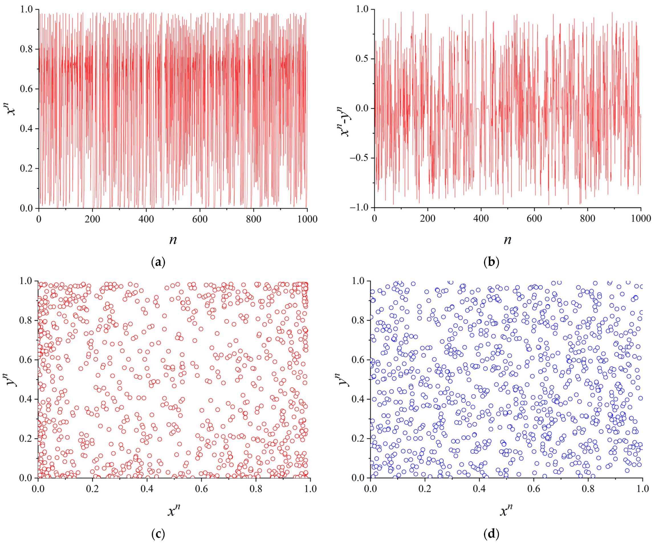
Improvement 1. In the initialization method, r₁, r₂, r₃, r₄ and q parameters of the standard HHO algorithm are all random methods, which will lead to the loss of representativeness of the CPP solution and poor network topology applicability. In order to reduce the shortage of small population diversity and slow the rate of convergence caused by the use of random initialization population, a Sin Chaos model with infinite fold times is introduced. Sin Chaos has the advantages of a fast rate of convergence, strong global search ability, and wide adaptability to engineering problems. The use of chaotic sequences for population initialization operation will affect the entire process of the algorithm, making the population more evenly distributed in the search space, enriching the diversity of initial solutions for global optimization, and thus improving the applicability of the solutions obtained from solving CPP. The Sin chaotic one-dimensional mapping equation is as follows:

$$\left\{\begin{array}{c}{\mathit{x}}_{\mathit{n}+1}=\frac{\alpha }{3}\sin (\pi x_{\mathit{n}}),n=0,1,\dots ,N\\ 0<\alpha \le 3\end{array}\right.$$

(27)

Figure 2a–c show the randomness, initial value sensitivity and ergodicity of the one-dimensional self-mapping after 1000 runs, and Figure 2d shows the population distribution using random initialization when α = 2.9512, x_n = 0.7555, y_n = 0.6555. It is indicated in Figure 2 that the improved population initialization generates more solution cases to be more conducive to global exploration.

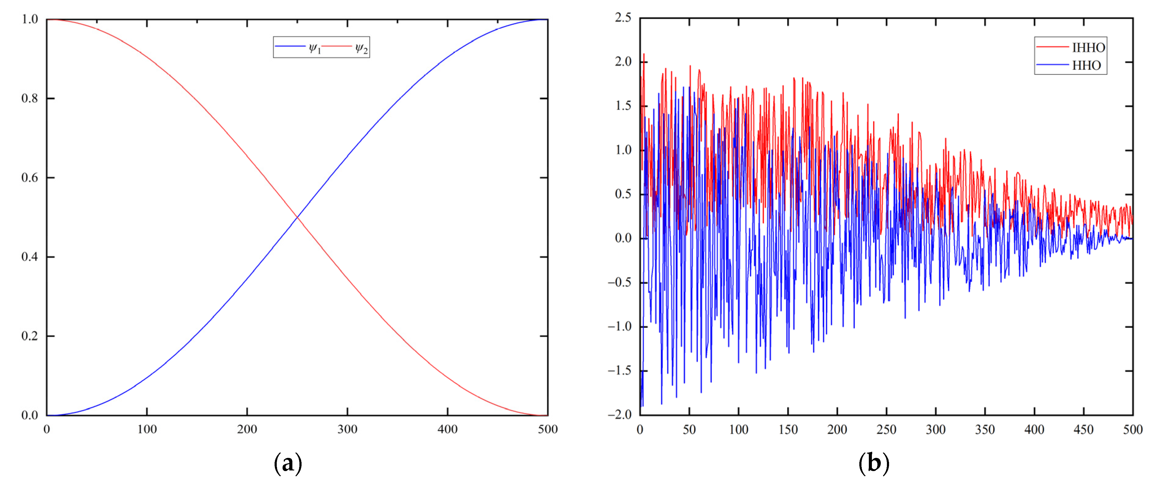
Improvement 2. The standard HHO algorithm only selects the optimal individual during the iteration process and does not communicate with other individuals. However, in order to solve CPP using multi-objective methods, selecting the optimal individual is often not the best choice, which can easily lead to limitations in the placement of the solved controller. The cosine function Cos is an even function that can be incremented or decremented under certain interval constraints and that has symmetry. It is very suitable for specific coefficients in swarm intelligence optimization algorithms for CPP solutions. The original random scaling coefficient r₁ is changed to Cos nonlinearly ${\psi }_1$ increasing to make the hawk swarm move toward the optimal position and achieve a more robust global search performance. As is shown in Figure 3a, the original scaling factor r₃ is changed to Cos nonlinear ${\psi }_2$, decreasing to speed up the algorithm’s convergence. To use the hypercube mechanism, replace X_rabbit(t), which is the current rabbit’s position, with the part of the guide X_leader utilizing the guide. The role of the guide X_leader is selected in such a way that one of the Harris hawks that is greater than the current mean value in the global repository REP is chosen as the guide. The average position X_m of the Harris hawk is improved by adding the part of the best global Harris hawk of the previous generation to reduce the risk that the algorithm is prone to fall into local optima. Related calculation equations are as follows:

$${\psi }_1=-\frac{\cos (\pi *\frac{-t}{T_{\max }})}{2}-1$$

(28)

$${\psi }_2=\frac{\cos (\pi *\frac{-t}{T_{\max }})}{2}+1$$

(29)

$$X_{leader}(t)=rand\left(REP(X_{rabbit}(\mathrm{t}))>\overline{\frac{p}{{\displaystyle \sum _{N\in REP}{e}^{-\beta N}}}}\right)$$

(30)

$$X_{mb}(t)=mean(X(t)))+X_{best}(t-1)$$

(31)

$$X(t+1)=\left\{\begin{array}{c}{X}_{\mathit{rand}}(t)-{\psi }_1|X_{rand}(t)-2r_{1}X(t)|\\ (X_{\mathit{leader}}(t)-(X_{\mathit{mb}}(t-1))-{\psi }_2(LB+r_2(UB-LB))\end{array}\right.\begin{array}{c}\\ \end{array}\begin{array}{c}q\ge 0.5\\ q<0.5\end{array}$$

(32)

Improvement 3. The size of prey energy E plays a vital role in regulating the global exploration and local exploitation. The smaller the E is, the more the HHO algorithm performs local exploitation, and the more significant the E is, the more the algorithm tends to perform global exploration. The basic HHO algorithm is too radical in the design of E, which does not conform to the way prey avoids pursuit in reality. In order to enhance the global search ability of the HHO algorithm, the prey escape energy E parameter is added to the dynamic adaptive weight $\omega$, which is composed of the cos function and the number of iterations T. The purpose is to make the switching between global exploration and local development smoother. The parameter design is based on experimental experience estimation. The iteration diagram of E is shown in Figure 3b. The $\omega$ and E can be calculated as follows:

$$\omega =1-\cos \left(\frac{-{\mathit{e}}^{2(1-\frac{t}{T})}-{\mathit{e}}^{-2(1-\frac{t}{T})}}{{\mathit{e}}^{2(1-\frac{t}{T})}+{\mathit{e}}^{-2(1-\frac{t}{T})}}\right)+\frac{1}{10}$$

(33)

$$E=\omega *4E_0,E_0\in (0,1)$$

(34)

Improvement 4. The switching between global search and local development in the basic HHO algorithm results in a reduced time sequence, leading to premature entry into local development and deviation from the target value in the early stage. Any local optimization is ineffective, and the global search is insufficient. As a result, the solved controller placement scheme cannot meet expectations, and the search group can randomly jump to a new area far from its current location. To check if there is a better target solution and achieve the effect of global development and reduce the deficiency of the HHO algorithm in the population diversity at the end of the iteration due to the decreasing time series, the Cauchy variation perturbation is added at the location of the optimal solution [38]. The peak of the Cauchy function is relatively small, and Harris hawk searches more for the global optimum after the Cauchy variation. Generating new solutions enhances the ability of the algorithm to leap out of the local space to check if a better CPP solution exists. The standard Cauchy distribution function is shown in Equation (35). The mathematical model of the Cauchy variation obtains the current global optimal solution, and X_{best_rabbit} updates the optimal solution with Equation (36).

$$f(x)=\frac{1}{\pi }(\frac{1}{x^2+1})$$

(35)

$$X_{bes\mathrm{t}\_rabbit}^{\prime }=X_{best\_rabbit}+X_{best\_rabbit}\otimes Cauchy(0,1)$$

(36)

5. A Multi-Controller Placement Strategy for SDN Based on the MOIHHO Algorithm

Reference [39] concluded through experimental analysis that, the number of network topology nodes should be fully considered, and the number of controllers placed should be within a reasonable range. Since the algorithm for CPP designed in this paper uses the in-band placement mode, the content of values for the number of controllers is set to no more than 30% of the network topology nodes. Each Harris hawk involved in the algorithm iteration represents a CPP placement scheme.

The placement strategy mainly consists of two stages, which are the construction stage of the objective function for CPP and the iterative solution stage for the CPP scheme. In the construction stage of the objective function for CPP, the main purpose is to convert the values of the three objective functions from specific mathematical models to code expressions that can participate in operations, consisting of a total of 29 steps. In the iterative solution stage for the CPP scheme, the main purpose is to obtain a certain number of CPP solutions within the limit of iteration times based on the value function composed of the previous three objective functions, including a total of 31 steps.

The pseudo-code of the proposed multi-controller placement strategy for SDN is demonstrated in Algorithm 1.

Algorithm 1 Multi-Controller Placement Strategy for SDN

1: undirected graph, link failure rate, city population, population size, maximum iteration number, dimension size, REP size, UB, LB. 2: Calculate the distance matrix between all nodes using Haversine Equation. 3: Construct a diagonal matrix according to the result of step 2. 4: Select the first K nodes as the initial local controller. 5: Use Equation (13) to calculate the reliability of all nodes. 6: for each i: Cloc do 7:    if other V Pr > Cloc Pr then 8:       Replace the initial local controller with an unselected node with higher reliability. 9:    end if 10:  end for 11: Equation (7) calculates the latency of all local controllers. 12: The node with the minimum sum of the results calculated in steps 5 and 6 is selected as the global controller. 13: Equation (11) was used to calculate the local controller’s maximum load value and actual load rate. 14: for each i = 1: N do 15:   for each j = 1: Lrat do 16:   Assign a switch whose value does not exceed the maximum negative value to each local controller. 17:    end for 18:  end for 19: Use Equation (10) to construct objective function 1. 20: Equation (14) is used to calculate the worst failure rate of the control link. 21: Use Equation (15) to calculate the failure rate in the controller domain of the local controller. 22: Equation (16) calculates the failure rate from the global controller to the local control. 23: Use Equation (17) to construct objective function 2. 24: Calculate the communication cost from the switch to the local controller and from the local controller to the global controller using Equation (18). 25: if Lact > Lrat then 26:    Equation (19) is used to calculate the processing cost of the local controller. 27:  end if 28: Calculate the flow processing placement cost using Equation (20). 29: Equation (21) is used to calculate objective function 3. 30: Construct the fitness function. 31: while K < 0.3*|V| do 32:    Initialize MOIHHO algorithm parameters. 33:    Use Equation (27) to initialize the position of the Harris hawk population. 34:    Calculate the fitness value of each Harris hawk. 35:    Set the Harris hawk position with the best fitness to the current prey position. 36:    Dominance assessment of all Harris hawks in the current population. 37:    Deposit the non-dominant Harris hawk into the Pareto front solution set REP. 38:    while it < MAXit do 39:       Use Equation (34) to update the escape energy of rabbits. 40:       for each (each hawk) do 41:       Select the facilitator using Equation (30). 42:           if E > 1 then 43:               Use Equation (32) to update the Harris position. 44:            end if 45:            if E < 1 then 46:               According to the position of the leader, four strategies of the standard HHO algorithm were used to update the part of the Harris hawk. 47:             end if 48:            Calculate the fitness value of each Harris hawk. 49:            Set the Harris hawk position with the best fitness as the prey position. 50:            Cauchy variation was applied according to Equation (36). 51:            Add a non-dominated solution to the REP library. 52:            Judge the dominance of new members. 53:            Store non-dominated solutions only in the REP library. 54:            if num (REP) > MAX (REP) then 55:               Delete a non-dominated solution. 56:             end if 57:       it = it + 1 58:    end for 59:    Output Pareto front solution set. 60:  K = K + 1 61:  end while 62:  return K CPP schemes

6. Simulation Experiments

The simulation experiment environment in this paper is shown in

Table 1. Hardware and software of the experimental environment.

Device	Parameter
simulation software	Matlab2020a
system software	Windows 11
CPU	Core i5 1135G7
RAM	16G
Hard drive	500G

, and the network topology is shown in

Table 2. Network topology information.

Network Topology	Number of Nodes	Number of Edges
ATT North America	25	56
China Telecom	38	62
IRIS Network	51	64

, using three large network topologies provided by the Topology Zoo website. ATT North America network is the next generation North American IP MPLS backbone network, China Telecom is a state-owned mega communications backbone enterprise network in China, and the IRIS network is a more than 5000-mile optical fiber network operating in Tennessee, USA. The classical Non-Dominated Sorting Genetic Algorithm II (NSGA-II) and the previously mentioned Multi-Objective Particle Swarm Algorithm (MOPSO) were used as comparison algorithms [40], the population size of the algorithm was 100, and the maximum number of iterations was set to 500, the REP size was set to 50 and other parameters were set as shown in

Table 3. Parameter Settings of the three algorithms.

MOPSO		NSGA-II		MOIHHO
Parameter Name	Value	Parameter Name	Value	Parameter Name	Value
Vmin	−4	Vmin	−5	LB	0
Vmax	4	Vmax	5	UB	1
w	0.5	Pcrossover	0.7	r1	rand
C1	1	Pmutation	0.4	r2	rand
C2	2			q	rand

, while the original values were used to set other parameters for selected algorithms.

Experiment 1. As shown in Figure 4a–c, the 50 sets of 3 objective function values obtained by the three algorithms were first assigned weights and then averaged to solve the index of the CPP scheme by each algorithm with the change in the number of controllers.

As is indicated in Figure 4, the average weighted values of the 50 CPP schemes solved by the three algorithms have a clear pattern. With the increase in the number of controllers, the average weighted values of the three indicators show a decreasing trend. Still, when the number of controllers reaches a specific number, the average weighted values of the three indicators begin to level off. They even appear to become more prominent again, which indicates that, for the same network topology, regardless of which algorithm is used to solve it, the number of controllers has an upper limit, not more but better. Using this rule, the number of controllers for the average weighted value of the three network topologies is slowed down simultaneously, which can be used as a reference for the analysis of the data in this paper. The use of the Pareto frontier to solve CPP does not mean that the number of other controllers placed is undesirable. For ATT North America topology, the number of local controllers is 5. For China Telecom topology, the number of local controllers is 7. For IRIS Network topology, the number of local controllers is 9.

Experiment 2. For the number of local controllers determined in Experiment 1, setting ${\lambda }_1$, ${\lambda }_2$ to 0.5 and average value Avg are counted for each of the three objectives, with worst latency $T_{worst}^{C_{loc}S}$ from the switch to the local controller, worst latency $T_{worst}^{C_{loc}{C}_{ove}}$ from the local controller to the global controller, average latency $T_{\mathrm{a}vg}^{C_{loc}S}$ from the switch to the local controller, average latency $T_{\mathrm{avg}}^{C_{loc}{C}_{ove}}$ from the local controller to the global controller, and average latency $T_{\mathrm{avg}}^{C_{loc}{C}_{ove}}$ from the local controller to the global controller. The placement reliability $R_{\mathrm{r}}^{C_{loc}}$ of all local controllers and the load variance average $L_{avg}$ of the optimal placement scheme are shown, respectively, in

Table 4. Indicators of ATT North America when the number of local controllers is 5.

Algorithms	Avg(T)	Avg(P)	Avg(C)	${\mathit{T}}_{\mathit{w}\mathit{o}\mathit{r}\mathit{s}\mathit{t}}^{{\mathit{C}}_{\mathit{l}\mathit{o}\mathit{c}}\mathit{S}}$	${\mathit{T}}_{\mathit{w}\mathit{o}\mathit{r}\mathit{s}\mathit{t}}^{{\mathit{C}}_{\mathit{l}\mathit{o}\mathit{c}}{\mathit{C}}_{\mathit{o}\mathit{v}\mathit{e}}}$	${\mathit{T}}_{\mathit{a}\mathit{v}\mathit{g}}^{{\mathit{C}}_{\mathit{l}\mathit{o}\mathit{c}}\mathit{S}}$	${\mathit{T}}_{\mathit{avg}}^{{\mathit{C}}_{\mathit{l}\mathit{o}\mathit{c}}{\mathit{C}}_{\mathit{o}\mathit{v}\mathit{e}}}$	${\mathit{R}}_{\mathit{r}}^{{\mathit{C}}_{\mathit{l}\mathit{o}\mathit{c}}}$	${\mathit{L}}_{\mathit{a}\mathit{v}\mathit{g}}$
MOIHHO	3.4295 × 10−3	1.6099 × 10−1	1.3928 × 103	2.2692 × 10−2	8.8446 × 10−3	1.2854 × 10−2	4.5710 × 10−3	3.4137 × 105	1.00
MOPSO	3.4285 × 10−3	1.4838 × 10−1	1.4108 × 103	2.2146 × 10−2	9.7017 × 10−3	1.4291 × 10−2	3.9884 × 10−3	3.2380 × 105	1.00
NSGA-II	3.6555 × 10−3	1.2429 × 10−1	1.5270 × 103	2.8998 × 10−2	1.0193 × 10−2	1.4423 × 10−2	5.2990 × 10−3	3.0115 × 105	1.00

,

Table 5. Indicators of China Telecom when the number of local controllers is 7.

Algorithms	Avg(T)	Avg(P)	Avg(C)	${\mathit{T}}_{\mathit{w}\mathit{o}\mathit{r}\mathit{s}\mathit{t}}^{{\mathit{C}}_{\mathit{l}\mathit{o}\mathit{c}}\mathit{S}}$	${\mathit{T}}_{\mathit{w}\mathit{o}\mathit{r}\mathit{s}\mathit{t}}^{{\mathit{C}}_{\mathit{l}\mathit{o}\mathit{c}}{\mathit{C}}_{\mathit{o}\mathit{v}\mathit{e}}}$	${\mathit{T}}_{\mathit{a}\mathit{v}\mathit{g}}^{{\mathit{C}}_{\mathit{l}\mathit{o}\mathit{c}}\mathit{S}}$	${\mathit{T}}_{\mathit{avg}}^{{\mathit{C}}_{\mathit{l}\mathit{o}\mathit{c}}{\mathit{C}}_{\mathit{o}\mathit{v}\mathit{e}}}$	${\mathit{R}}_{\mathit{r}}^{{\mathit{C}}_{\mathit{l}\mathit{o}\mathit{c}}}$	${\mathit{L}}_{\mathit{a}\mathit{v}\mathit{g}}$
MOIHHO	3.2438 × 10−3	1.6476 × 10−1	2.9412 × 103	2.9969 × 10−2	5.5100 × 10−3	1.9482 × 10−2	3.0558 × 10−3	2.6642 × 105	0.42
MOPSO	3.2944 × 10−3	1.7203 × 10−1	3.0272 × 103	3.2137 × 10−2	7.3276 × 10−3	2.2678 × 10−2	3.5304 × 10−3	2.5726 × 105	0.51
NSGA-II	3.3524 × 10−3	1.5468 × 10−1	3.0529 × 103	3.4424 × 10−2	8.9033 × 10−3	1.9357 × 10−2	3.5344 × 10−3	2.7567 × 105	0.58

and

Table 6. Indicators of IRIS Network when the number of local controllers is 9.

Algorithms	Avg(T)	Avg(P)	Avg(C)	${\mathit{T}}_{\mathit{w}\mathit{o}\mathit{r}\mathit{s}\mathit{t}}^{{\mathit{C}}_{\mathit{l}\mathit{o}\mathit{c}}\mathit{S}}$	${\mathit{T}}_{\mathit{w}\mathit{o}\mathit{r}\mathit{s}\mathit{t}}^{{\mathit{C}}_{\mathit{l}\mathit{o}\mathit{c}}{\mathit{C}}_{\mathit{o}\mathit{v}\mathit{e}}}$	${\mathit{T}}_{\mathit{a}\mathit{v}\mathit{g}}^{{\mathit{C}}_{\mathit{l}\mathit{o}\mathit{c}}\mathit{S}}$	${\mathit{T}}_{\mathit{avg}}^{{\mathit{C}}_{\mathit{l}\mathit{o}\mathit{c}}{\mathit{C}}_{\mathit{o}\mathit{v}\mathit{e}}}$	${\mathit{R}}_{\mathit{r}}^{{\mathit{C}}_{\mathit{l}\mathit{o}\mathit{c}}}$	${\mathit{L}}_{\mathit{a}\mathit{v}\mathit{g}}$
MOIHHO	4.7974 × 10−4	1.6616 × 10−1	4.4529 × 102	4.1951 × 10−3	1.5919 × 10−3	2.1252 × 10−3	7.4584 × 10−4	3.6167 × 106	1.66
MOPSO	5.4759 × 10−4	1.7120 × 10−1	5.1486 × 102	4.4450 × 10−3	1.7742 × 10−3	2.6907 × 10−3	6.8275 × 10−4	3.1383 × 106	1.85
NSGA-II	5.0761 × 10−4	1.6564 × 10−1	4.5089 × 102	5.5358 × 10−3	1.3451 × 10−3	2.1839 × 10−3	6.6406 × 10−4	3.3131 × 106	1.73

.

According to the values of the three objective functions T, P and C in Table 4, it can be found that the target values obtained by the three algorithms are very similar for the ATT North America topology with 25 network nodes and 56 edges. It shows that the proposed solution of multi-controller strategy based on the MOIHHO algorithm for SDN can achieve the same level of mature multi-objective optimization algorithm effect. As indicated in Table 5, in the China Telecom network topology with 38 nodes and 62 edges, the target value solved by the MOIHHO algorithm gradually becomes advantageous in some indicators, especially in Avg(T), Avg(P) and Avg(C), compared with the solution result of NSGA-II. As shown in Table 6, in the IRIS Network topology with 51 nodes and 64 edges, the triple objective values solved by the MOIHHO algorithm are better than MOPSO and NSGA-II in most of the metrics, which achieves better results as the number of nodes in the network topology gradually increases and the size of the network becomes more extensive and more complex.

Comparing the three SDN network topologies, the evaluation metrics, such as worst latency, average latency, reliability, load value and overhead, commonly used in the CPP research field, are combined. Further analysis of the data in Table 4, Table 5 and Table 6 shows that, compared to the CPP scheme of the MOPSO algorithm, the CPP scheme of MOIHHO reduces the worst latency from the switch to the local controller by about 8%. The average latency from the switch to the local controller increases by about 15%, the reliability of local controller placement increases by about 10%, and the average value of load variance reduces by about 20%. The average value of the combined placement overhead is reduced by 10%. Compared with the CPP scheme of the NSGA-II algorithm, the CPP scheme of MOIHHO reduces the worst latency from the switch to the local controller by about 20%, the average latency by about 5%, the placement reliability of the local controller increases by about 7% and the average load variance decreases by about 13%. The average combined placement overhead reduces by about 14%.

Figure 5 provides the multi-controller placement for hierarchical management of SDN in three large network topologies solved by the MOIHHO algorithm.

As shown in Figure 5, it can be seen intuitively that the local controllers are placed on the nodes with extensive access, and the global controllers are also placed on the nodes with complete access, which confirms that using node reliability to place controllers is very effective. The location of the global controller is in the middle of all three network topologies, which is in line with the expected results. Similarly, observing the mapping relationship between switches and local controllers, the vast majority of the mapping relationships do not have the problem of cross-domain communication. For NP hard problems like CPP, it is acceptable to sacrifice part of the network performance to ensure load balancing. Still, the effect of cross-domain communication is minimal for the CPP scheme solved by the MOIHHO algorithm, in which it can be found that the mapping of local controllers to switches does not exceed a distance of, at most, two hops by observing the placement diagram.

7. Conclusions and Future Work

Based on symmetric/asymmetric structures in the SDN architecture, this paper considers the CPP problem for hierarchical management of SDN as a multi-objective optimization problem. Four improvements are made to address the shortcomings of the basic HHO algorithm, and a multi-controller placement strategy based on the MOIHHO is proposed. The placement of multi-controllers and the mapping relationship between switches and local controllers are solved from network-integrated latency, link-integrated failure rate, node reliability and integrated overhead. Through experimental simulations of three real large-scale SDN topologies, the strategy proposed in this paper can obtain a multi-controller placement strategy for the hierarchical management of SDN with more negligible integrated latency, higher reliability and smaller overhead while maintaining load balancing. The experimental comparison with two representative multi-objective algorithms (NSGA-II and MOPSO) shows that, as the network topology increases in size and the link situation becomes more complex, the CPP scheme obtained by the MOIHHO algorithm achieves better results in terms of integrated latency, integrated reliability and integrated placement overhead. The proposed strategy in this paper is more robust and has better adaptability to the network topology, and can provide better ideas and research reference value for the practical application of large-scale SDN network topology.

In the next step, considering our prior work in application scenarios of network intrusion detection [41,42] and, at the same time, according to symmetric/asymmetric structures in SDN, the optimization index in this paper will be further improved to solve the CPP that meets the application scenario of security management for SDN. As for future work, in terms of reliability, intrusion detection will be combined with dynamic placement of controllers in order to seek a more stable CPP solution and, in terms of flow processing strategies, collaboration with network operators with actual addresses will be promoted in order to obtain a more realistic scale of network node traffic and enhance the data reliability of the model designed in this paper.

References

1. Nunes, B.A.A.; Mendonca, M.; Nguyen, X.N.; Obraczka, K.; Turletti, T. A survey of software-defined networking: Past, present, and future of programmable networks. IEEE Commun. Surv. Tutor. 2014, 16, 1617–1634. [Google Scholar] [CrossRef] [Green Version]
2. Foundation, O.N. Software-Defined Networking: The New Norm for Networks. Available online: https://opennetworking.org/sdn-resources/whitepapers/software-defined-networking-the-new-norm-for-networks (accessed on 9 October 2013).
3. Singh, A.K.; Maurya, S.; Kumar, N.; Srivastava, S. Heuristic approaches for the reliable SDN controller placement problem. Trans. Emerg. Telecommun. Technol. 2020, 31, e3761. [Google Scholar] [CrossRef]
4. Rajoriya, M.K.; Gupta, C.P. A taxonomy on distributed controllers in software defined networking. In Proceedings of the 5th International Conference on Computing Methodologies and Communication, ICCMC 2021, Erode, India, 8–10 April 2021; pp. 120–126. [Google Scholar]
5. Tootoonchian, A.; Ganjali, Y. HyperFlow: A distributed control plane for openFlow. In Proceedings of the 2010 Internet Network Management Conference on Research on Enterprise Networking, San Jose, CA, USA, 27 April 2010. [Google Scholar]
6. Hassas Yeganeh, S.; Ganjali, Y. Kandoo: A framework for efficient and scalable offloading of control applications. In Proceedings of the First Workshop on Hot Topics in Software Defined Networks, New York, NY, USA, 13 August 2012; pp. 19–24. [Google Scholar]
7. Schütz, G.; Martins, J.A. A comprehensive approach for optimizing controller placement in software-defined networks. Comput. Commun. 2020, 159, 198–205. [Google Scholar] [CrossRef]
8. Cui, J.; Lu, Q.; Zhong, H.; Tian, M.; Liu, L. A load-balancing mechanism for distributed SDN control plane using response time. IEEE Trans. Netw. Serv. Manag. 2018, 15, 1197–1206. [Google Scholar] [CrossRef] [Green Version]
9. Heller, B.; Sherwood, R.; McKeown, N. The controller placement problem. In Proceedings of the First Workshop on Hot Topics in Software Defined Networks, New York, NY, USA, 13 August 2012; pp. 7–12. [Google Scholar]
10. Alowa, A.; Fevens, T. Towards minimum inter-controller delay time in software defined networking. Procedia Comput. Sci. 2020, 175, 395–402. [Google Scholar] [CrossRef]
11. Kurra, C.; Janyani, V.; Battula, R.B. FANIC: Farthest node initialization clustering technique for controller placement problem in software defined networking. In Proceedings of the 2020 International Conference on Artificial Intelligence and Signal Processing, AISP 2020, Amaravati, India, 10–12 January 2020. [Google Scholar]
12. Alhazmi, K.; Moubayed, A.; Shami, A. Distributed SDN controller placement using betweenness centrality & hierarchical clustering. In Proceedings of the 8th ACM Symposium on Design and Analysis of Intelligent Vehicular Networks and Applications, Montreal, QC, Canada, 25 October–2 November 2018; pp. 15–20. [Google Scholar]
13. Zhang, Q.; Li, H.; Liu, Y.; Ouyang, S.; Fang, C.; Mu, W.; Gao, H. A new quantum particle swarm optimization algorithm for controller placement problem in software-defined networking. Comput. Electr. Eng. 2021, 95, 107456. [Google Scholar] [CrossRef]
14. Hock, D.; Hartmann, M.; Gebert, S.; Jarschel, M.; Zinner, T.; Tran-Gia, P. Pareto-optimal resilient controller placement in SDN-based core networks. In Proceedings of the 2013 25th International Teletraffic Congress, Shanghai, China, 10–12 September 2013; pp. 1–9. [Google Scholar]
15. Ahmadi, V.; Khorramizadeh, M. An adaptive heuristic for multi-objective controller placement in software-defined networks. Comput. Electr. Eng. 2018, 66, 204–228. [Google Scholar] [CrossRef]
16. Wang, Z.; Li, Y.; Guan, S. A robust-link controller placement model for large-scale software defined networks. Trans. Emerg. Telecommun. Technol. 2023, 34, e4765. [Google Scholar] [CrossRef]
17. Firouz, N.; Masdari, M.; Sangar, A.B.; Majidzadeh, K. A hybrid multi-objective algorithm for imbalanced controller placement in software-defined networks. J. Netw. Syst. Manag. 2022, 30, 51. [Google Scholar] [CrossRef]
18. Schmid, S.; Suomela, J. Exploiting locality in distributed SDN control. In Proceedings of the Second ACM SIGCOMM Workshop on Hot Topics in Software Defined Networking, Hong Kong, China, 16 August 2013; pp. 121–126. [Google Scholar]
19. Oktian, Y.E.; Lee, S.G.; Lee, H.J.; Lam, J.H. Distributed SDN controller system: A survey on design choice. Comput. Netw. 2017, 121, 100–111. [Google Scholar] [CrossRef]
20. Hussain, M.; Shah, N.; Amin, R.; Alshamrani, S.S.; Alotaibi, A.; Raza, S.M. Software-defined networking: Categories, analysis, and future directions. Sensors 2022, 22, 5551. [Google Scholar] [CrossRef] [PubMed]
21. Heidari, A.A.; Mirjalili, S.; Faris, H.; Aljarah, I.; Mafarja, M.; Chen, H. Harris hawks optimization: Algorithm and applications. Future Gener. Comput. Syst. 2019, 97, 849–872. [Google Scholar] [CrossRef]
22. Guo, W.; Xu, P.; Dai, F.; Zhao, F.; Wu, M. Improved Harris hawks optimization algorithm based on random unscented sigma point mutation strategy. Appl. Soft Comput. 2021, 113, 108012. [Google Scholar] [CrossRef]
23. Basha, J.; Bacanin, N.; Vukobrat, N.; Zivkovic, M.; Venkatachalam, K.; Hubálovský, S.; Trojovský, P. Chaotic harris hawks optimization with quasi-reflection-based learning: An application to enhance CNN design. Sensors 2021, 21, 6654. [Google Scholar] [CrossRef]
24. Killi, B.P.R.; Rao, S.V. Controller placement in software defined networks: A comprehensive survey. Comput. Netw. 2019, 163, 106883. [Google Scholar] [CrossRef]
25. Priyadarsini, M.; Bera, P. Software defined networking architecture, traffic management, security, and placement: A survey. Comput. Netw. 2021, 192, 108047. [Google Scholar] [CrossRef]
26. Jalili, A.; Keshtgari, M.; Akbari, R.; Javidan, R. Multi criteria analysis of controller placement problem in software defined networks. Comput. Commun. 2019, 133, 115–128. [Google Scholar] [CrossRef]
27. Kumari, A.; Sairam, A.S. Controller placement problem in software-defined networking: A survey. Networks 2021, 78, 195–223. [Google Scholar] [CrossRef]
28. Yu, M.; Rexford, J.; Freedman, M.J.; Wang, J. Scalable flow-based networking with DIFANE. In Proceedings of the ACM SIGCOMM 2010 Conference on SIGCOMM, New Delhi, India, 30 August–3 September 2010; pp. 351–362. [Google Scholar]
29. SINGH, A.K.; MAURYA, S.; SRIVASTAVA, S. Varna-based optimization: A novel method for capacitated controller placement problem in SDN. Front. Comput. Sci. 2020, 14, 143402. [Google Scholar] [CrossRef]
30. Thajeel, T.G.; Abdulhassan, A. A comprehensive survey on software-defined networking load balancers. In Proceedings of the 4th International Iraqi Conference on Engineering Technology and Their Applications, IICETA 2021, Najaf, Iraq, 21 September 2021; pp. 1–7. [Google Scholar]
31. Wang, C.A.; Hu, B.; Chen, S.Z.; Li, D.S.; Liu, B. A switch migration-based decision-making scheme for balancing load in SDN. IEEE Access 2017, 5, 4537–4544. [Google Scholar] [CrossRef]
32. Zhang, B.; Wang, X.W.; Huang, M. Multi-objective optimization controller placement problem in internet-oriented software defined network. Comput. Commun. 2018, 123, 24–35. [Google Scholar] [CrossRef]
33. Khorramizadeh, M.; Ahmadi, V. Capacity and load-aware software-defined network controller placement in heterogeneous environments. Comput. Commun. 2018, 129, 226–247. [Google Scholar] [CrossRef]
34. Zhao, Z.; Wu, B. Scalable SDN architecture with distributed placement of controllers for WAN. Concurr. Comput. Pract. Exp. 2017, 29, e4030. [Google Scholar] [CrossRef]
35. Qu, C.; He, W.; Peng, X.; Peng, X. Harris hawks optimization with information exchange. Appl. Math. Model. 2020, 84, 52–75. [Google Scholar] [CrossRef]
36. Coello Coello, C.A.; Lechuga, M.S. MOPSO: A proposal for multiple objective particle swarm optimization. In Proceedings of the 2002 Congress on Evolutionary Computation, Honolulu, HI, USA, 12–17 May 2002; pp. 1051–1056. [Google Scholar]
37. Knowles, J.D.; Corne, D.W. Approximating the nondominated front using the Pareto archived evolution strategy. Evol. Comput. 2000, 8, 149–172. [Google Scholar] [CrossRef] [PubMed]
38. Anil Kumar, K.R.; Dhas, E.R. Opposition based genetic optimization algorithm with Cauchy mutation for job shop scheduling problem. Mater. Today Proc. 2022, 72, 3006–3011. [Google Scholar] [CrossRef]
39. Hu, Y.; Wang, W.; Gong, X.; Que, X.; Cheng, S. On reliability-optimized controller placement for software-defined networks. China Commun. 2014, 11, 38–54. [Google Scholar] [CrossRef]
40. Deb, K.; Agrawal, S.; Pratap, A.; Meyarivan, T. A fast elitist non-dominated sorting genetic algorithm for multi-objective optimization: NSGA-II. In Proceedings of the International Conference on Parallel Problem Solving from Nature, Berlin, Germany, 18–20 September 2000; pp. 849–858. [Google Scholar]
41. Xu, H.; Przystupa, K.; Fang, C.; Marciniak, A.; Kochan, O.; Beshley, M. A combination strategy of feature selection based on an integrated optimization algorithm and weighted k-nearest neighbor to improve the performance of network intrusion detection. Electronics 2020, 9, 1206. [Google Scholar] [CrossRef]
42. Xu, H.; Lu, Y.; Guo, Q. Application of improved butterfly optimization algorithm combined with black widow optimization in feature selection of network intrusion detection. Electronics 2022, 11, 3531. [Google Scholar] [CrossRef]
Figure 1. The thinking of hierarchical management for SDN by multi-controller placement.
Symmetry 15 01520 g001
Figure 2. (ac) are the randomness, initial value sensitivity, and ergodicity of Sin Chaos initialization and (d) is the ergodicity of random initialization.
Symmetry 15 01520 g002
Figure 3. (a) is the variation curve of ψ 1 and ψ 2 ; (b) is the iterative plot of the escape capacity E.
Symmetry 15 01520 g003
Figure 4. (a) is the ATT North America topology; (b) is the China Telecom topology; (c) is the IRIS Network topology.
Symmetry 15 01520 g004aSymmetry 15 01520 g004b
Figure 5. (a) is the ATT North America topology; (b) is the China telecom topology; (c) is the IRIS Network topology.
Symmetry 15 01520 g005aSymmetry 15 01520 g005b