


A Novel Fractional-Order Memristive Chaotic Circuit with Coexisting Double-Layout Four-Scroll Attractors and Its Application in Visually Meaningful Image Encryption


Abstract
1. Introduction
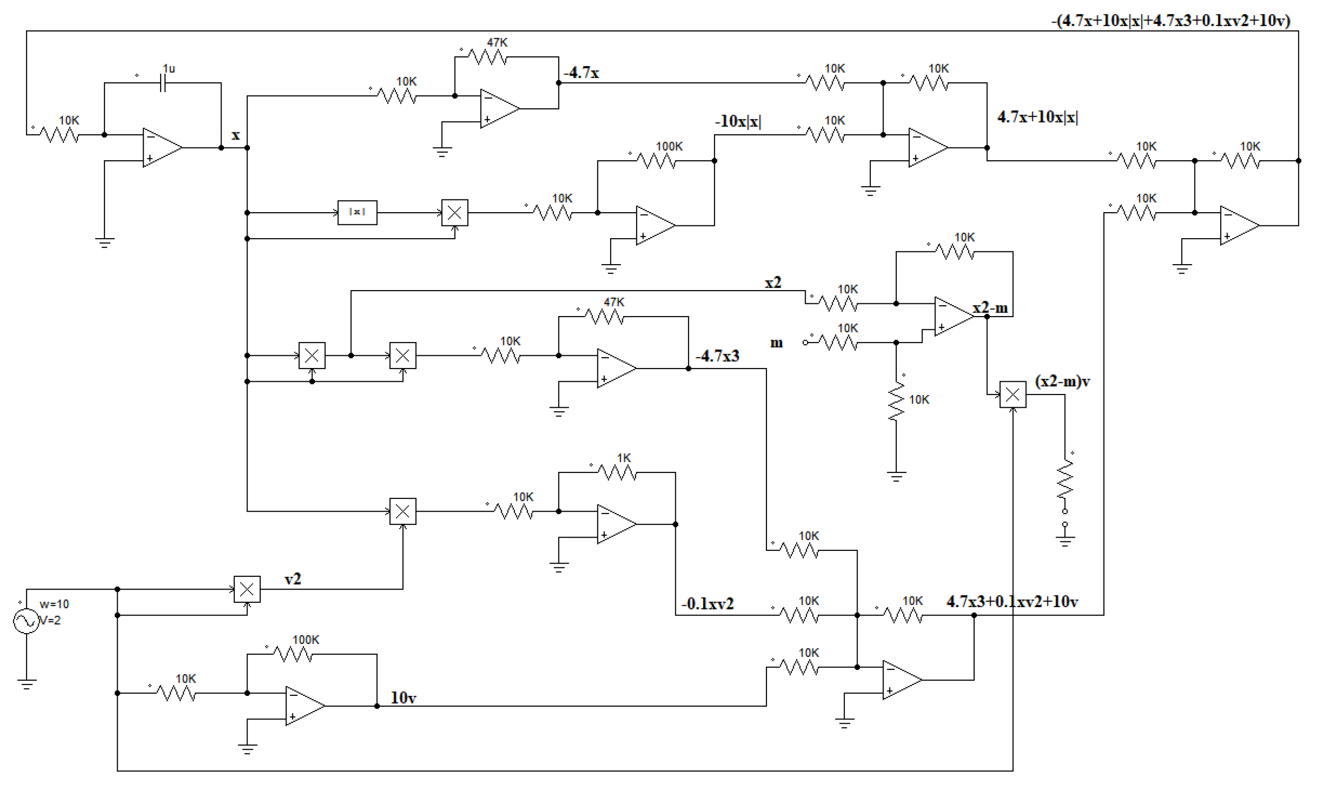
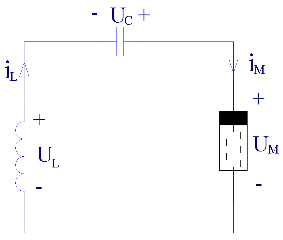
2. New Locally Active Memristor
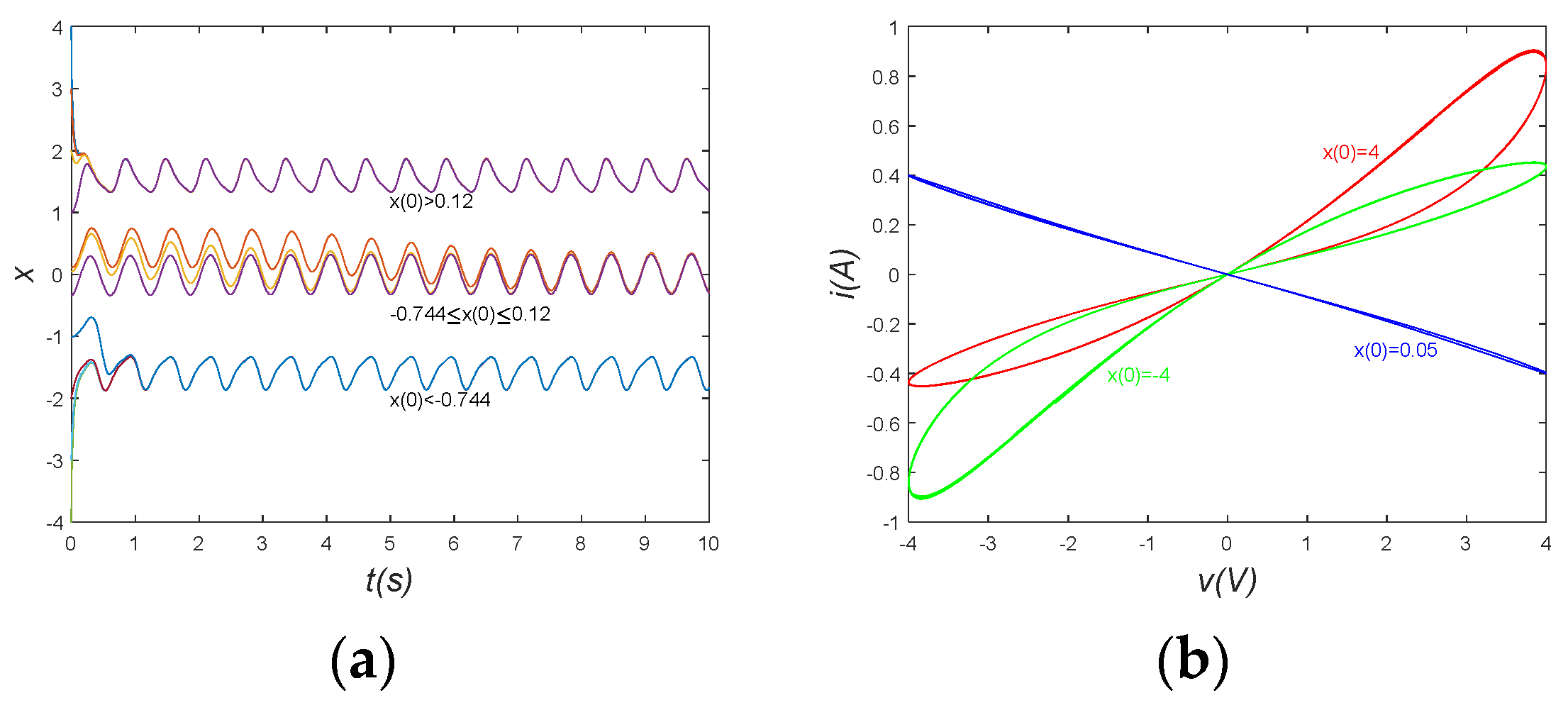
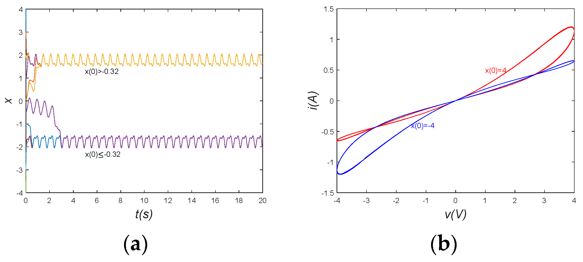
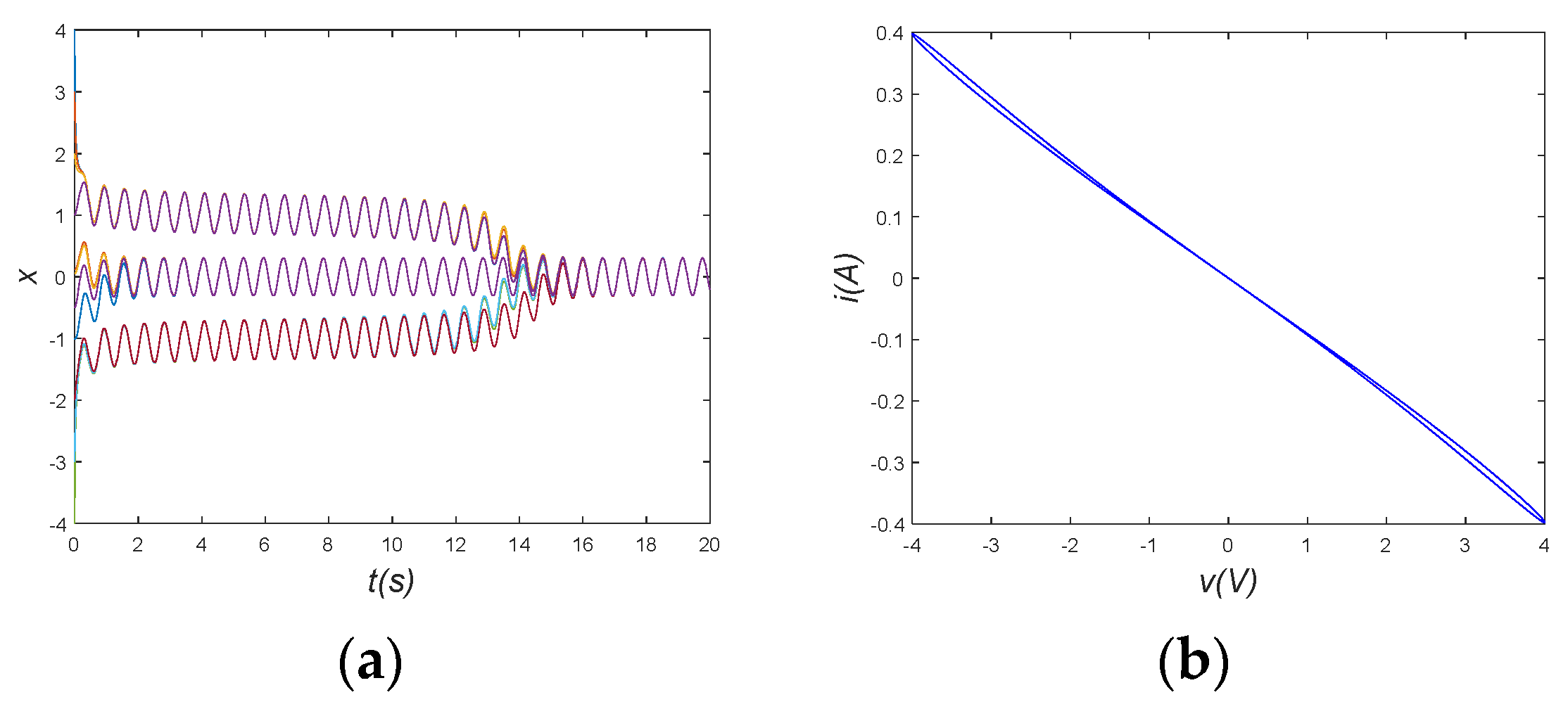
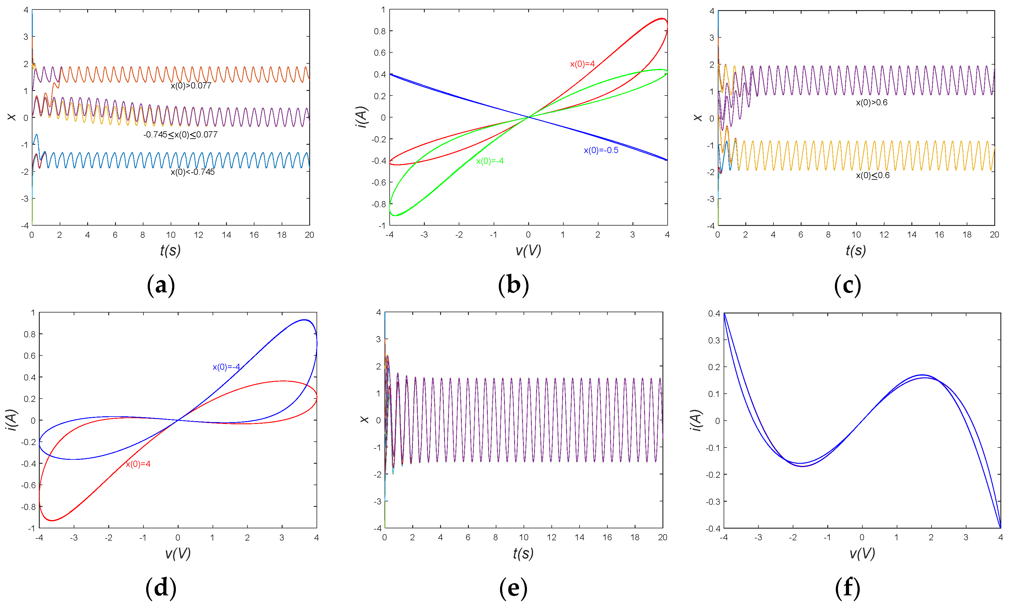
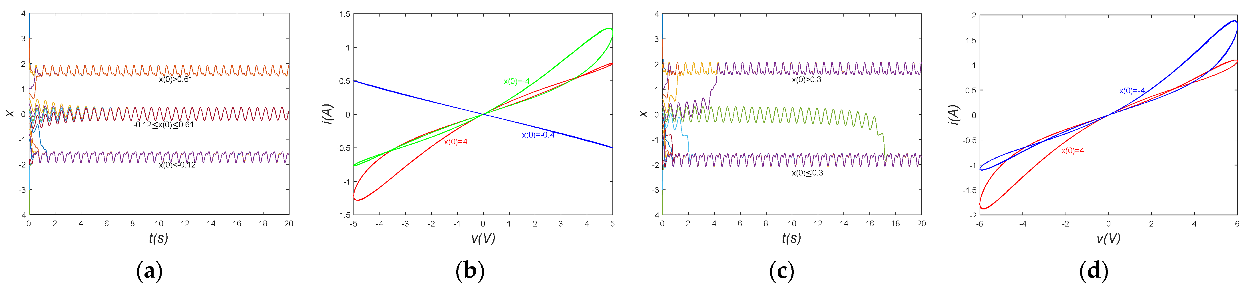
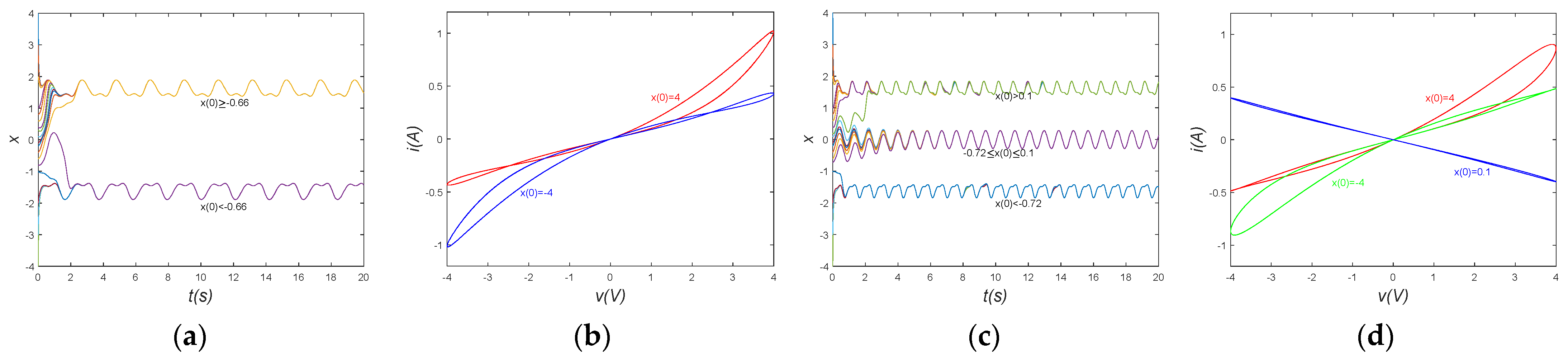
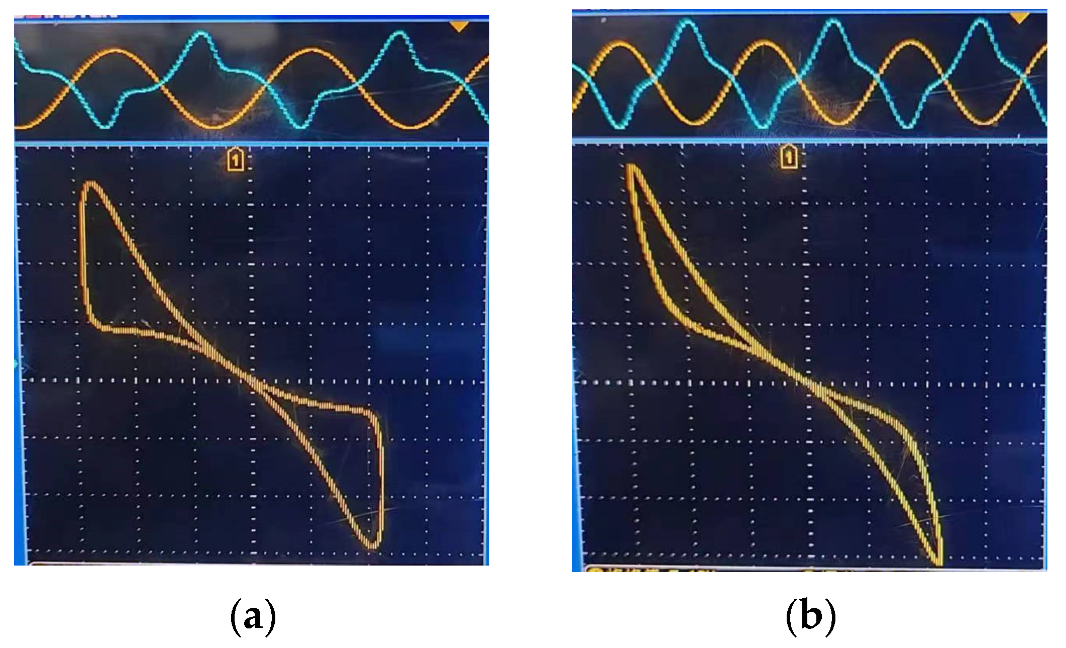
2.1. Pinched Hysteresis Loops
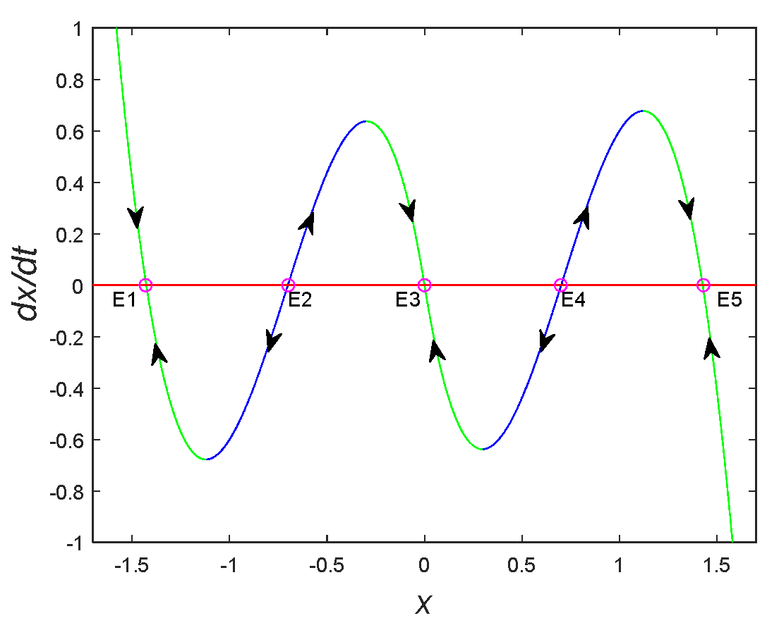
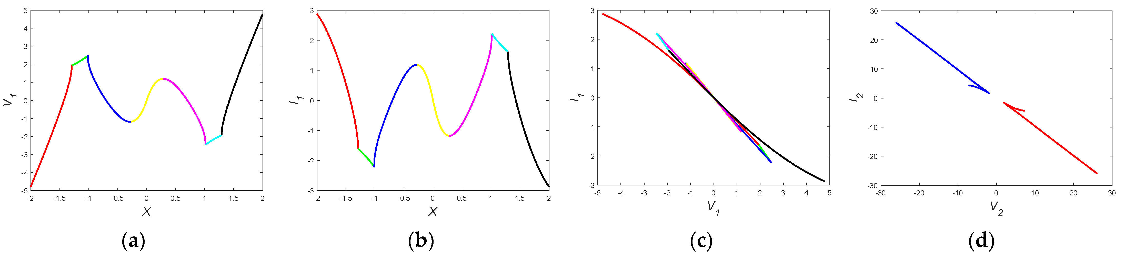
2.2. Local Activity
3. Fractional-Order Memristive Chaotic System
3.1. Fractional Calculus
3.2. The Stability of the System
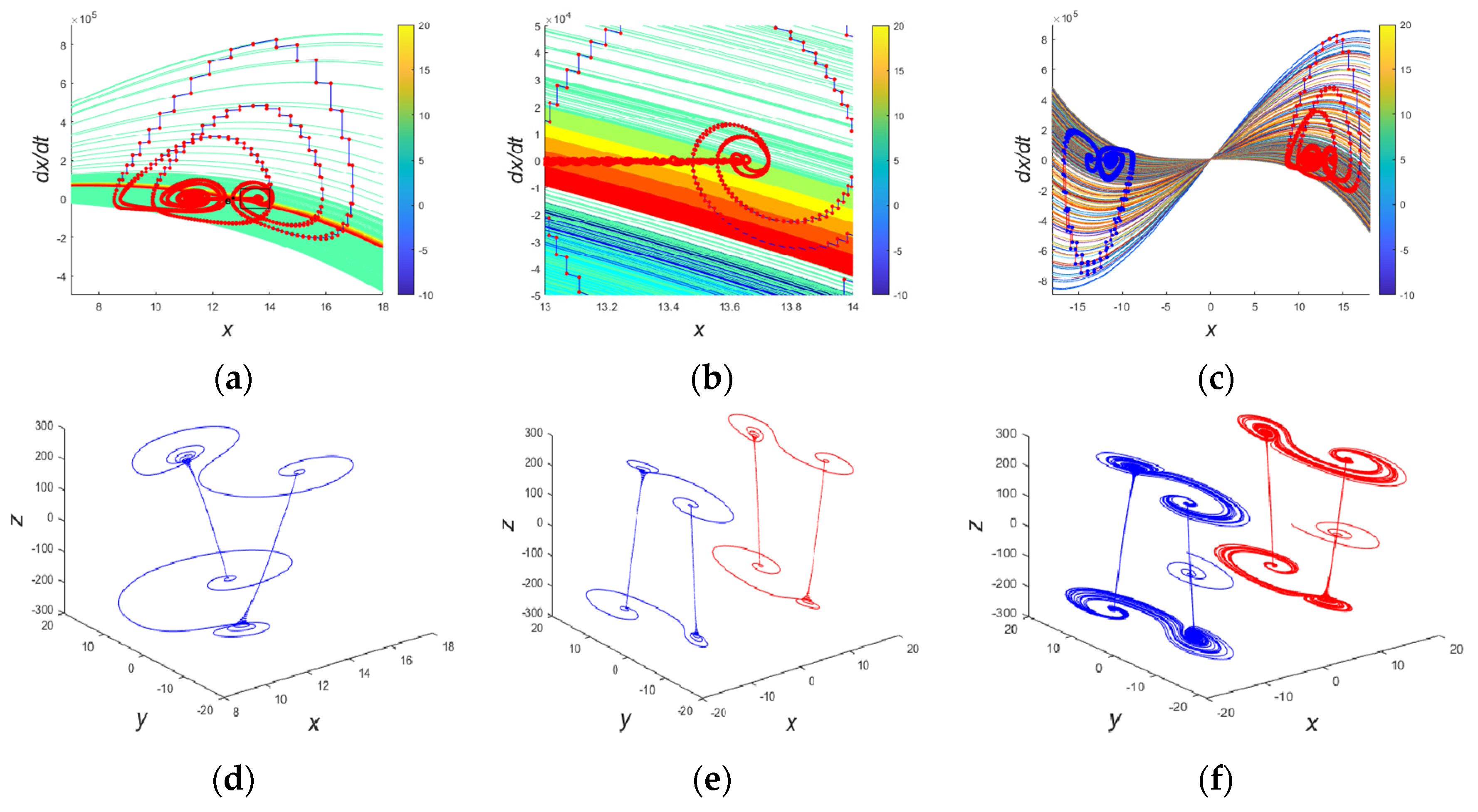
3.3. Mechanism of Chaotic Oscillation
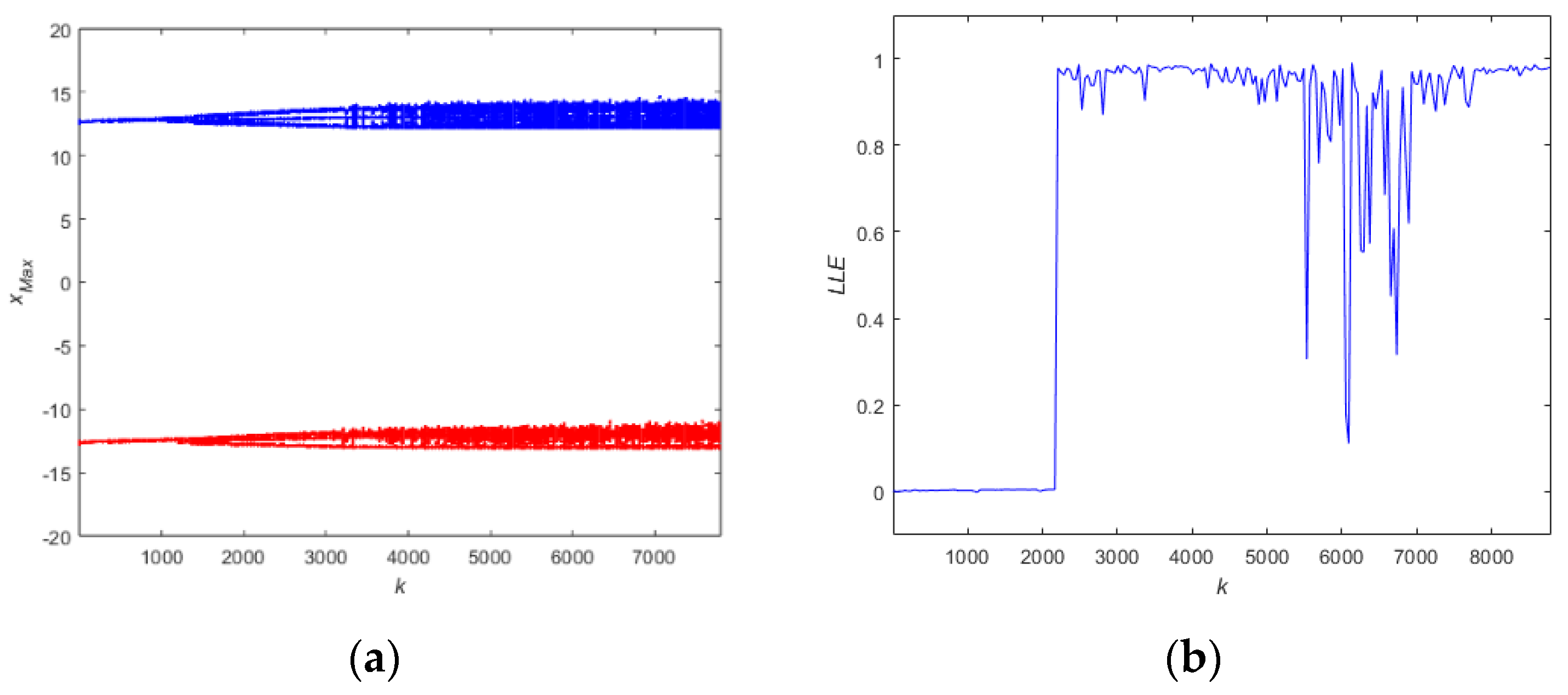
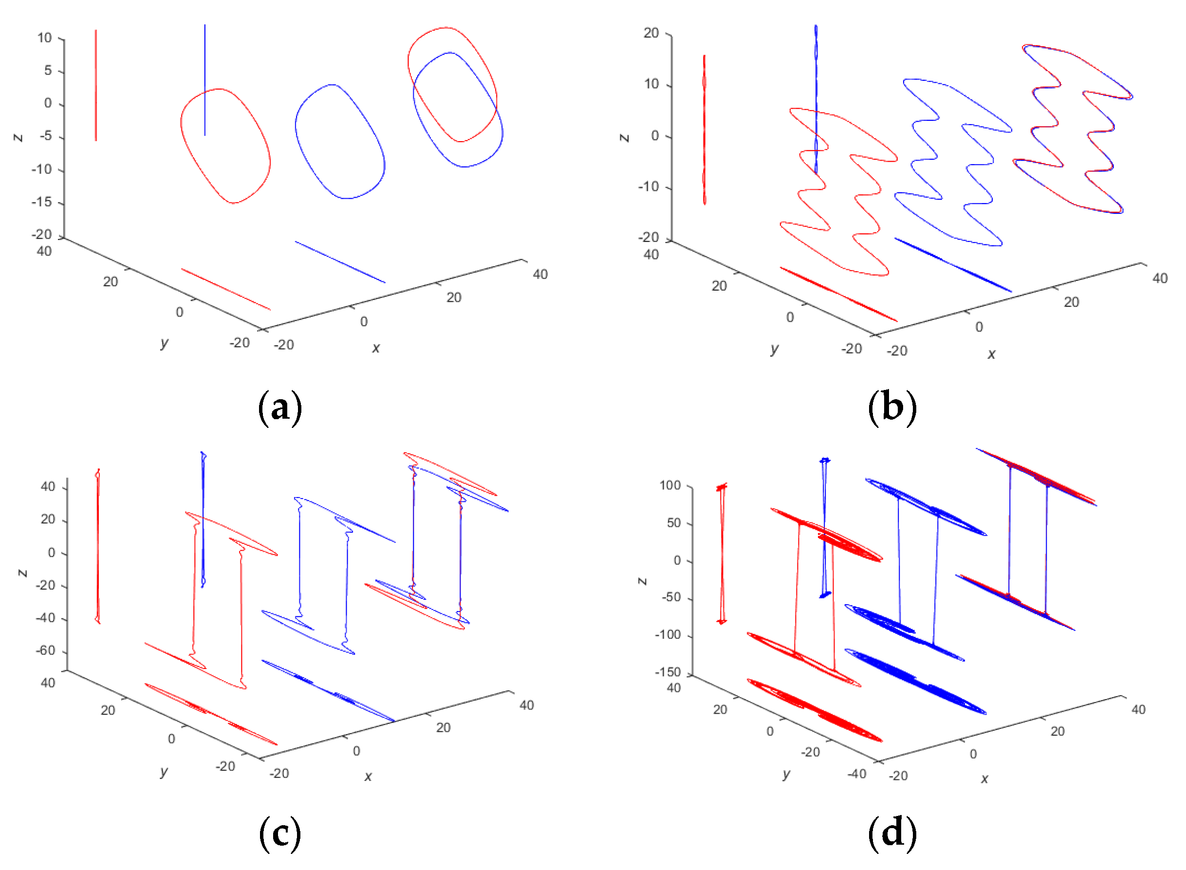
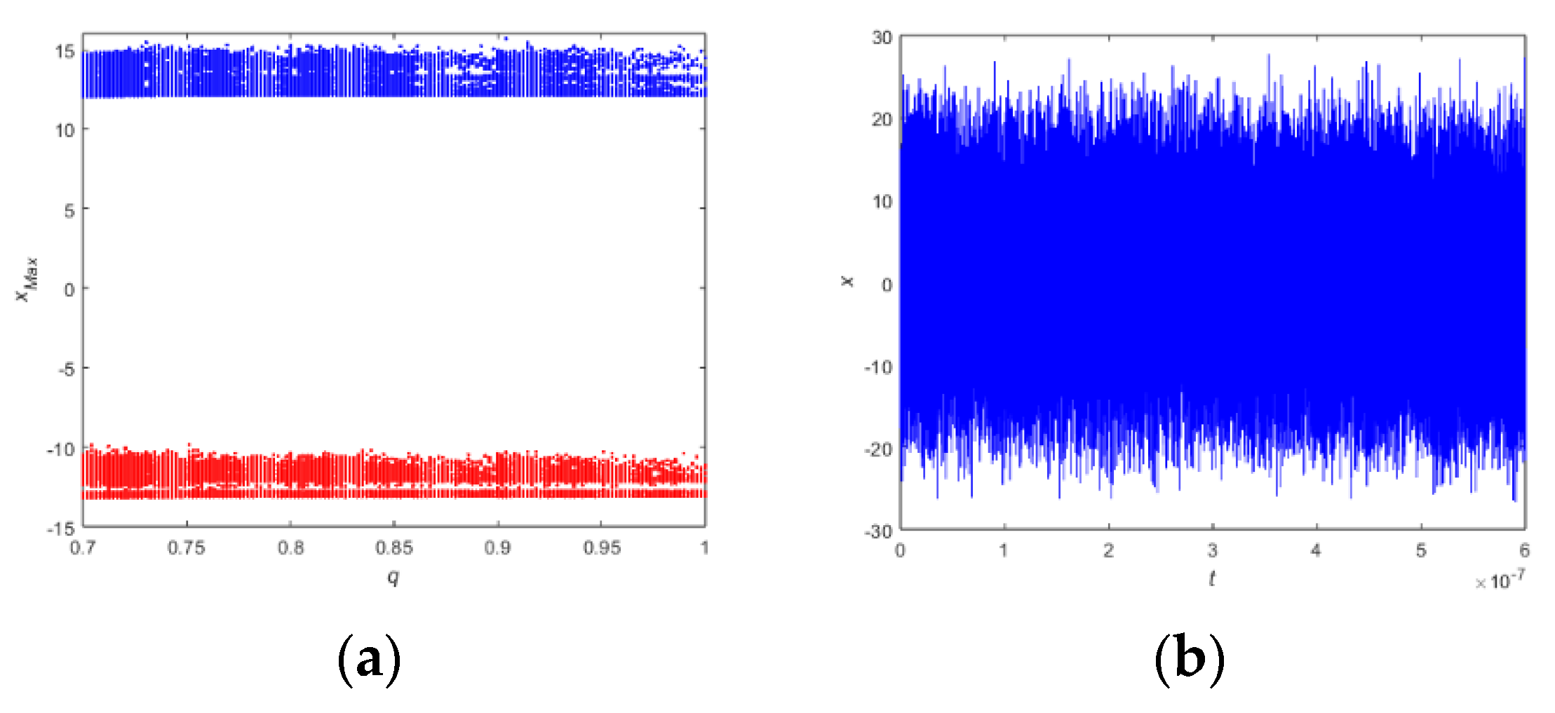
3.4. Dynamic Behaviors
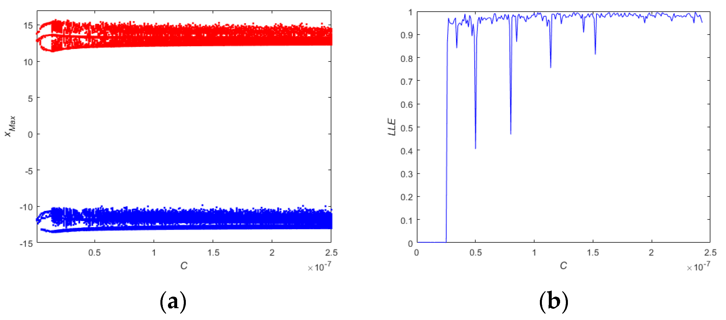
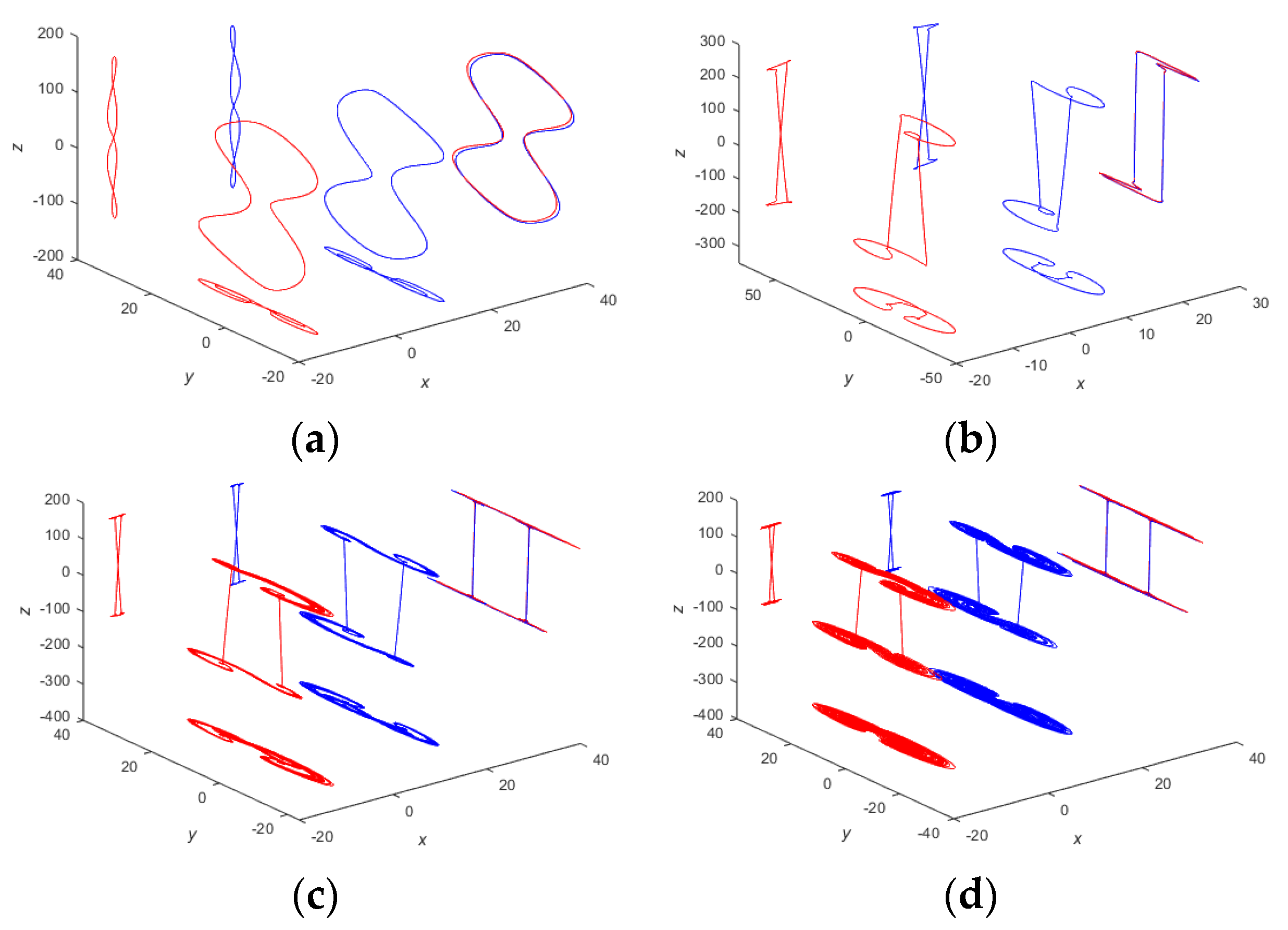
3.4.1. Dynamic Depending on
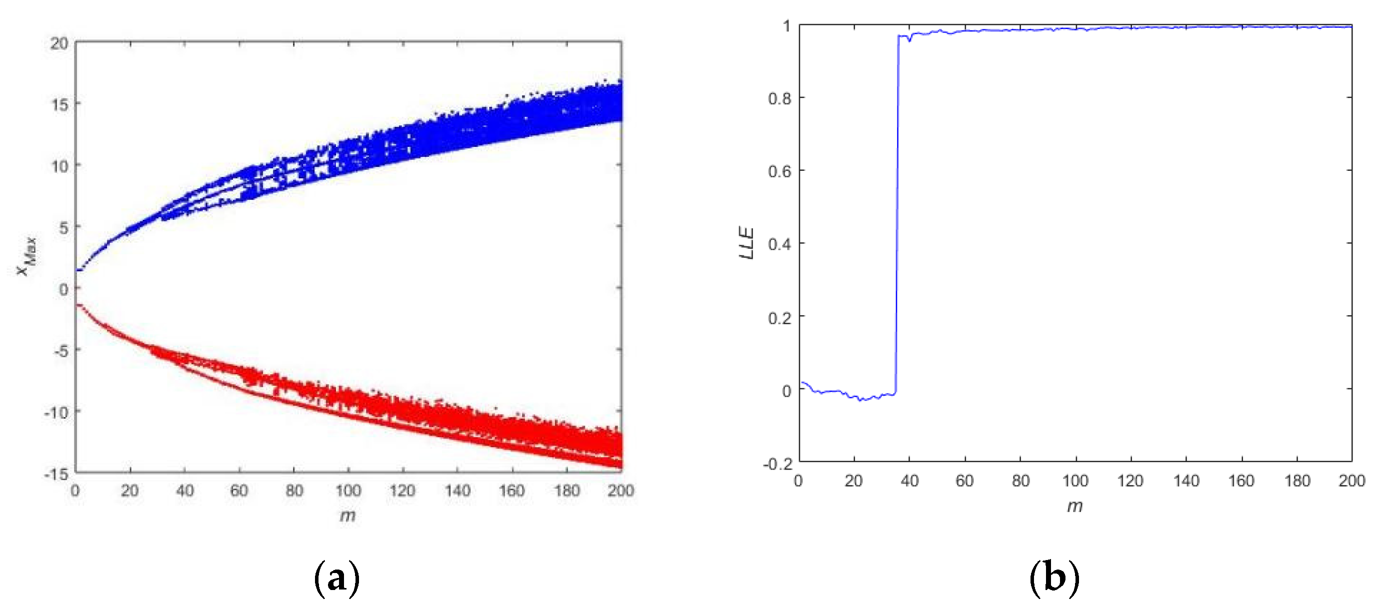
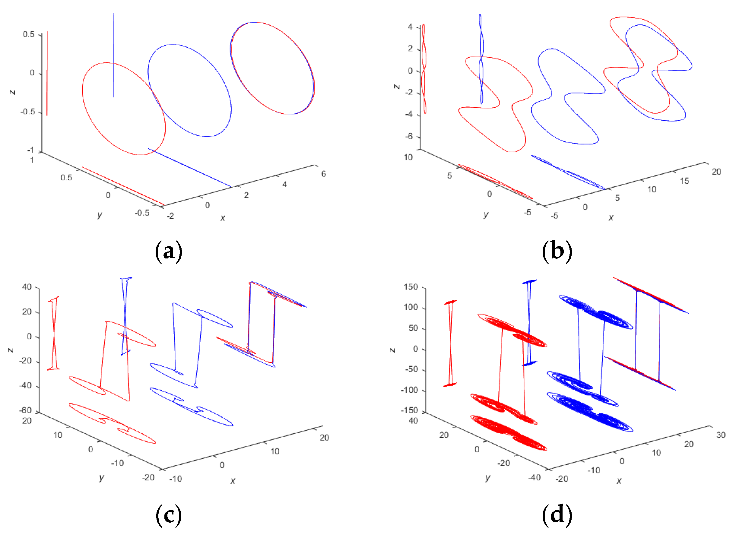
3.4.2. Dynamic Depending on
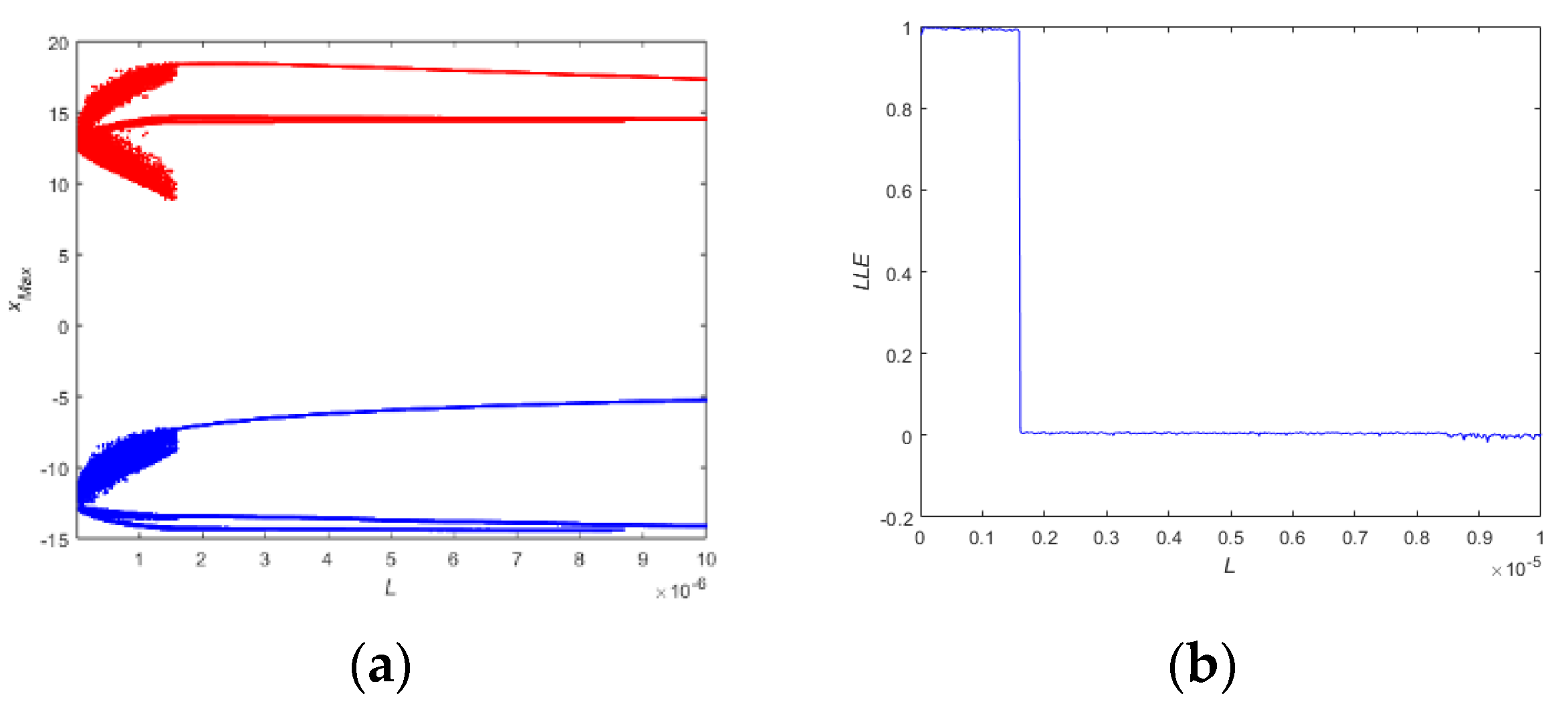
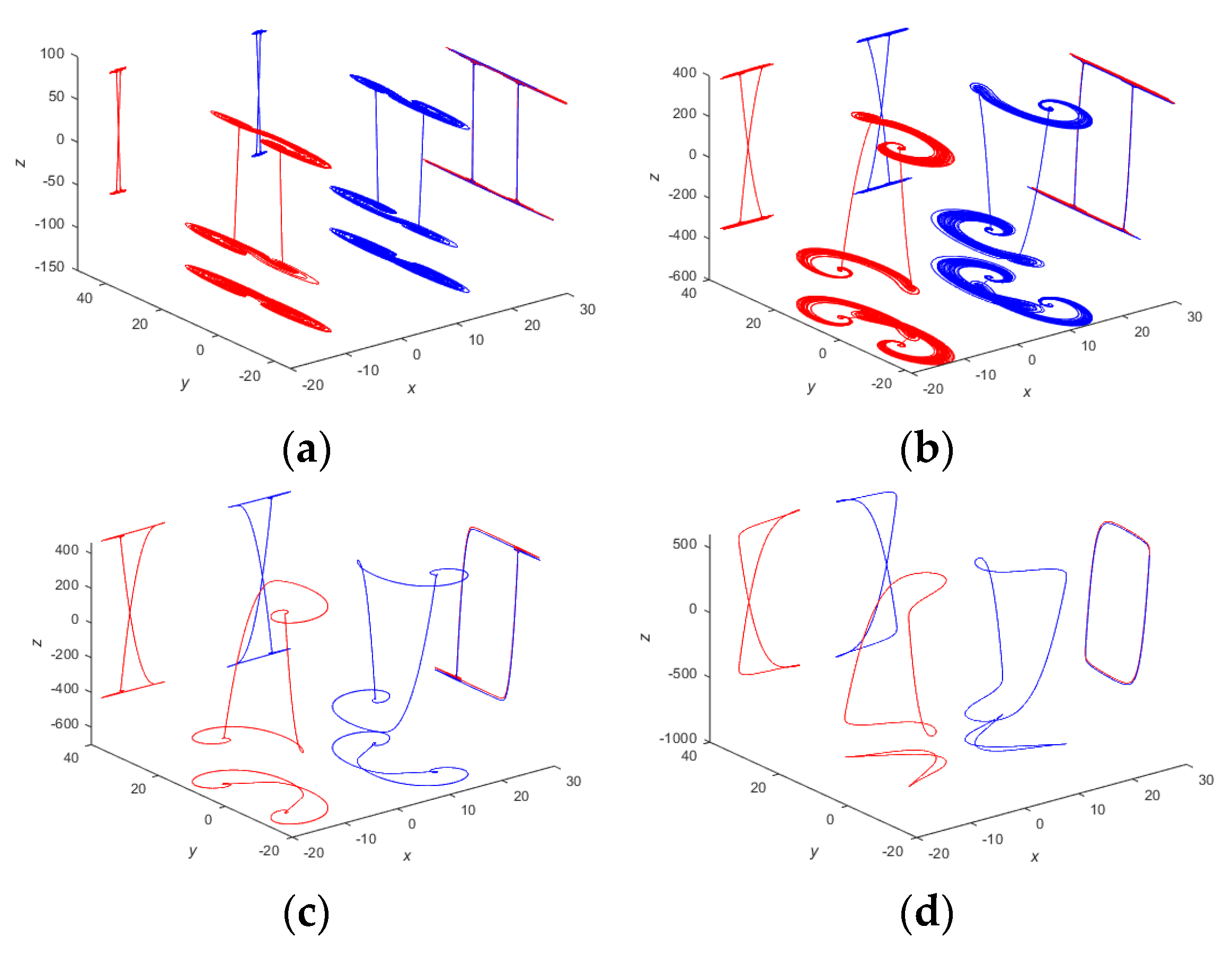
3.4.3. Dynamic Depending on
3.4.4. Dynamic Depending on
3.4.5. Dynamic Depending on
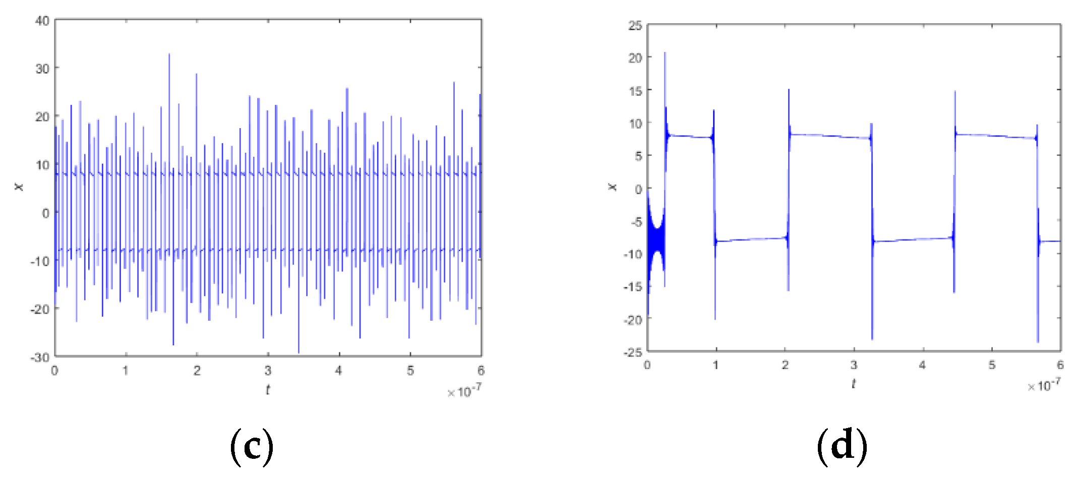
3.5. Complexity Analysis
4. Visually Meaningful Image Encryption and Decryption Scheme
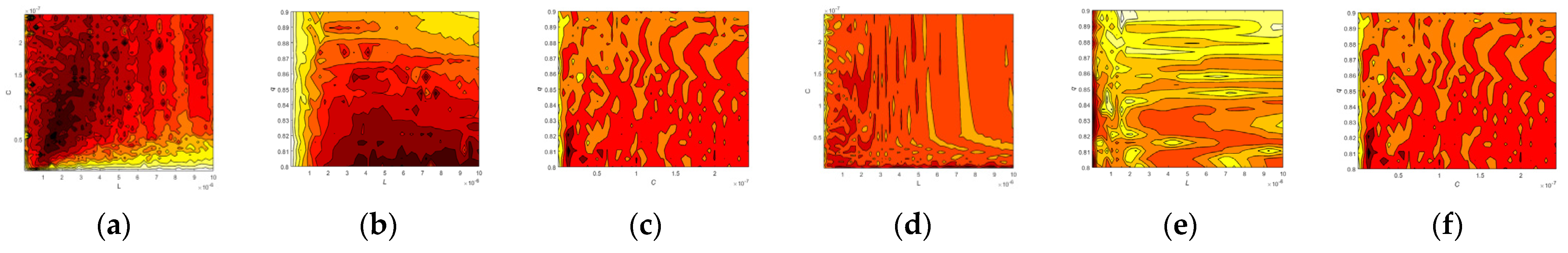
4.1. Chaotic Sequence Generation
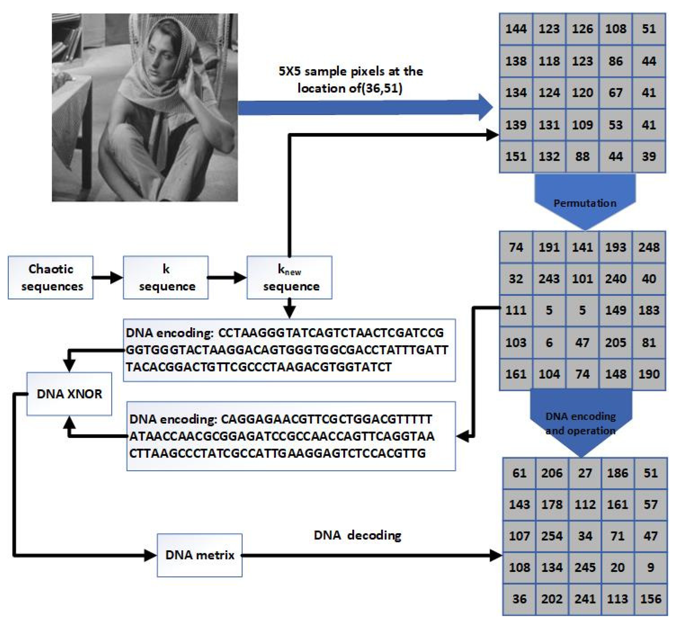
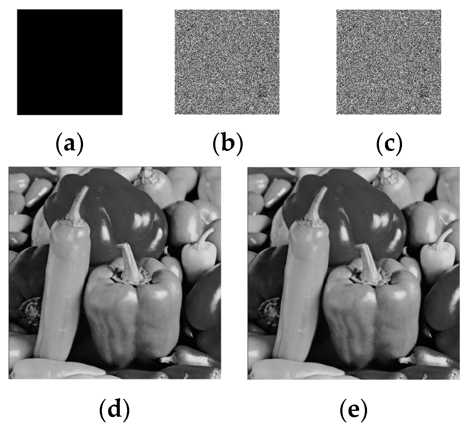
4.2. Image Encryption
| Algorithm 1: The image encryption process. |
| (1) Convert into a binary matrix |
| (2) Convert into a binary sequence |
| (3) Arrange the sequence order, and acquire a new sequence |
| (4) for i = 1:mn × 8 do |
| (i) = ((i)) |
| End for |
| (5) Encode the sequence as a DNA sequence using the eighth DNA encoding rule |
| (6) Transform the sequence into a binary sequence |
| (7) Encode the sequence as a DNA sequence using the first DNA encoding rule |
| (8) for i = 1:mn × 4 do |
| End for |
| (9) Extract the odd term of sequence as a new sequence |
| (10) Transform the sequence into the sequence on the value of |
| (11) Decode the sequence to a binary sequence using the fourth DNA encoding rule |
| (12) Convert binary sequence into decimal matrix |
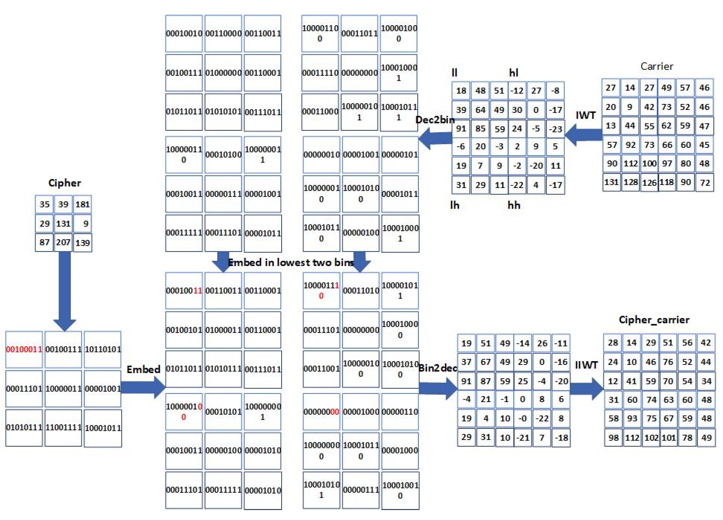
4.3. Cipher Image Embedding Process
| Algorithm 2: The cipher embedding process. |
| (1) Decompose the carrier image by IWT, and then transform it into the sequences , , , |
| (2) Transform , , , as 8-bit binary sequences , , , |
| (3) Convert the secret image into 8-bit binary sequence |
| (4) Replace the lowest 2 bits of , , , with the bits of |
| (5) = [(:,1:6), (:,1:2)] |
| (6) = [(:,1:6), (:,3:4)] |
| (7) = [(:,1:6), (:,5:6)] |
| (8) = [(:,1:6), (:,7:8)] |
| (9) Transform the sequences , , , into decimal sequences , , , |
| (10) Use inverse IWT to convert , , , into a visually meaningful cipher image |
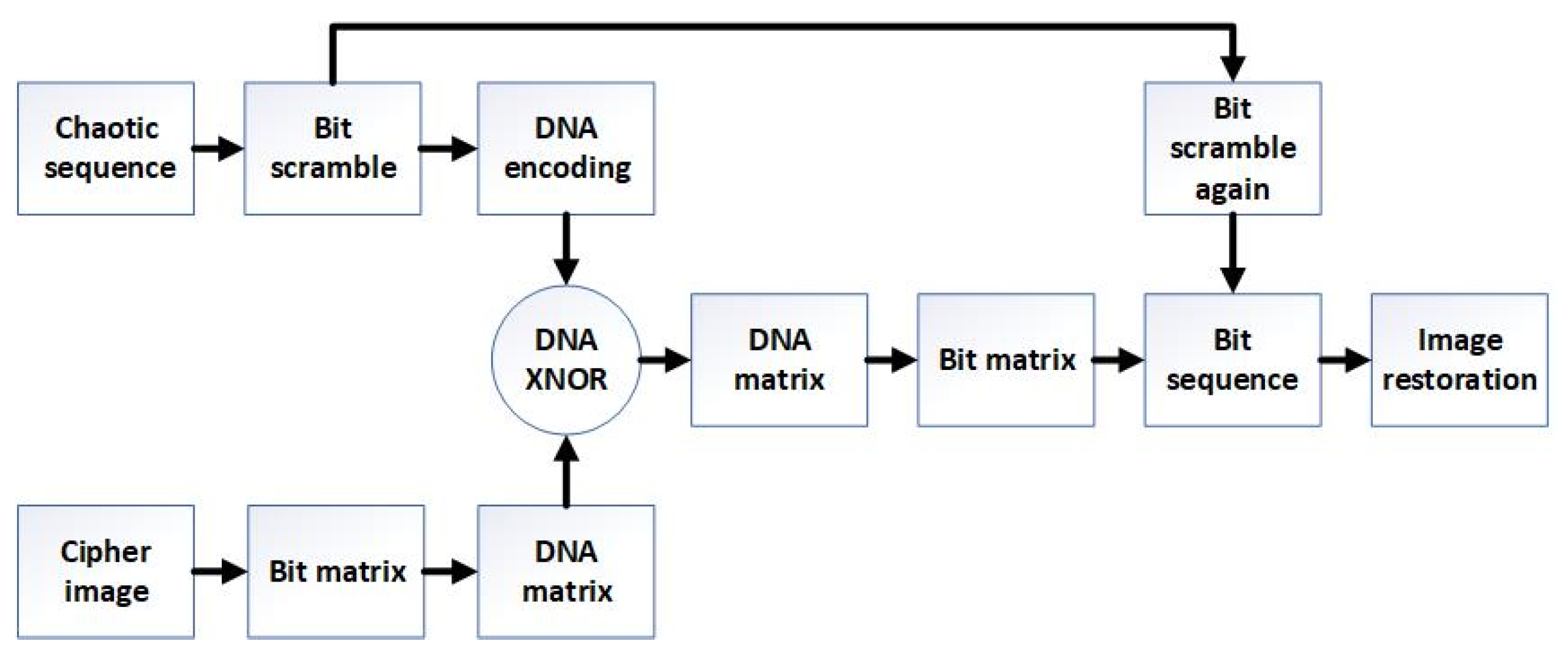
4.4. Image Decryption Scheme
4.5. Extracting the Cipher Image
5. Numerical Simulation and Analysis
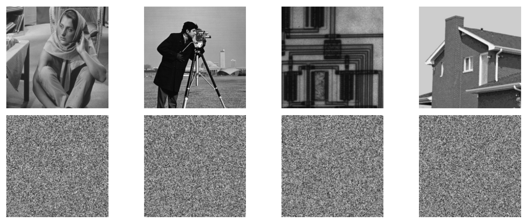
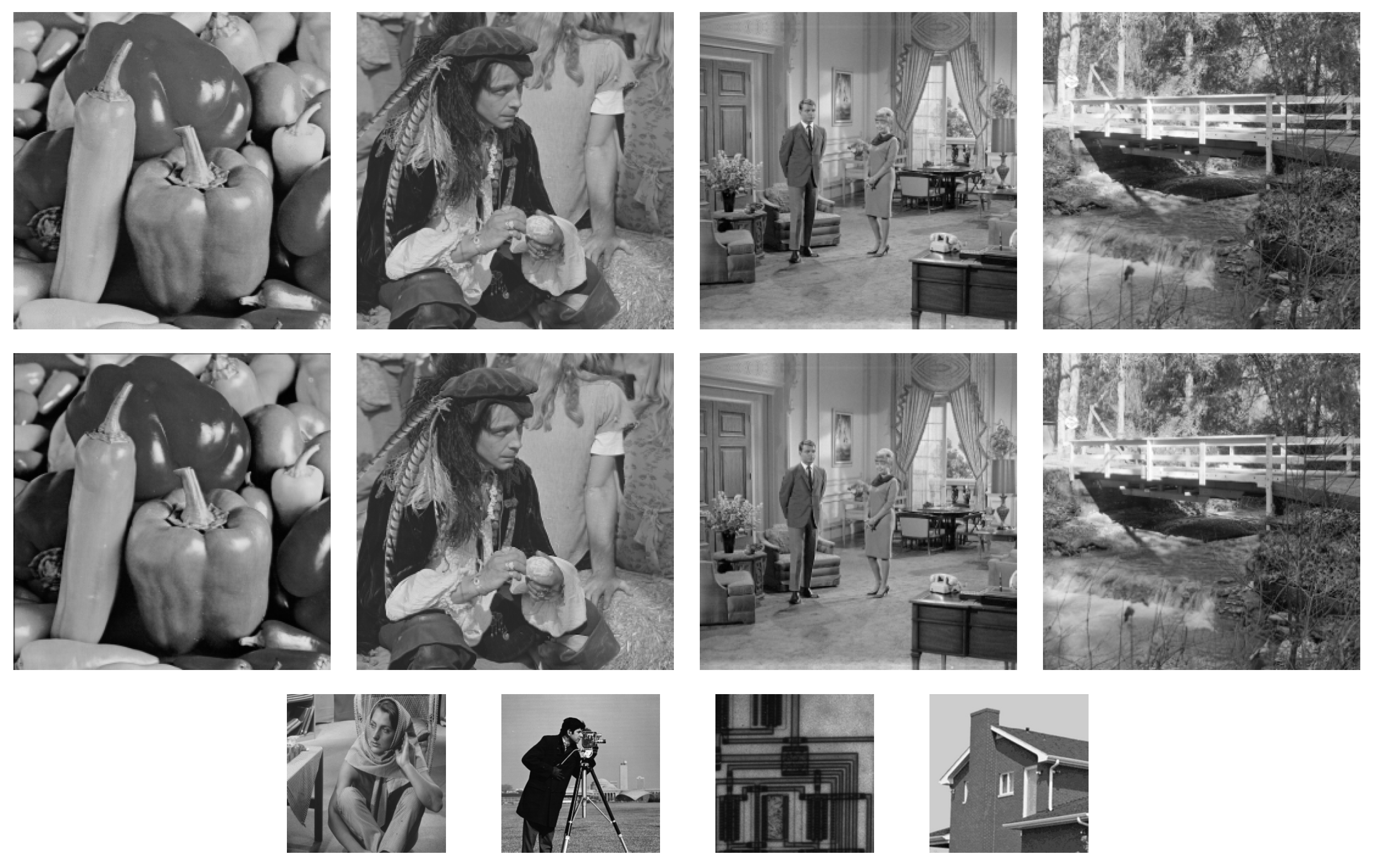
5.1. Simulated Results
5.2. Performance Analyses
5.2.1. Key Security Analysis
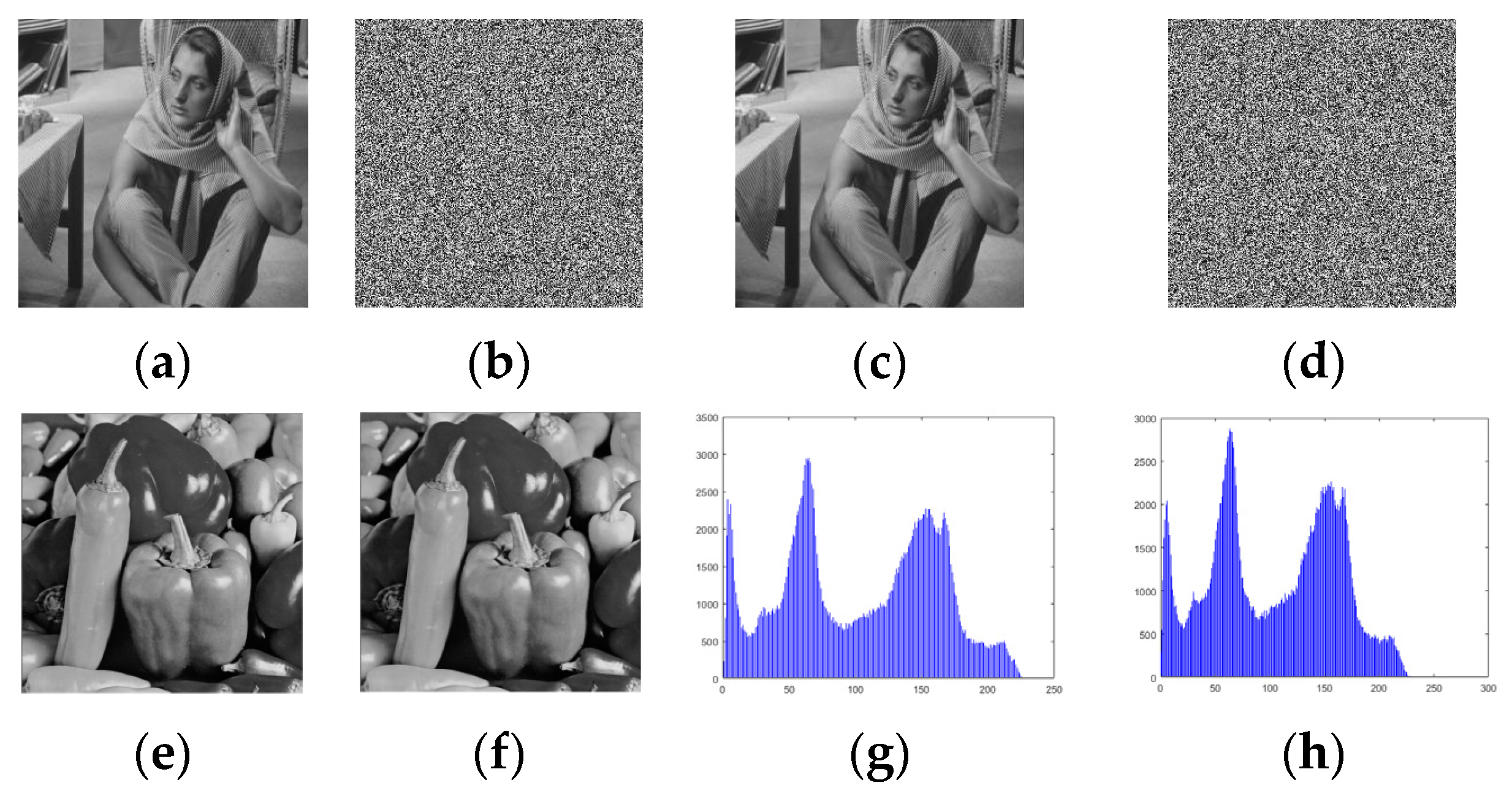
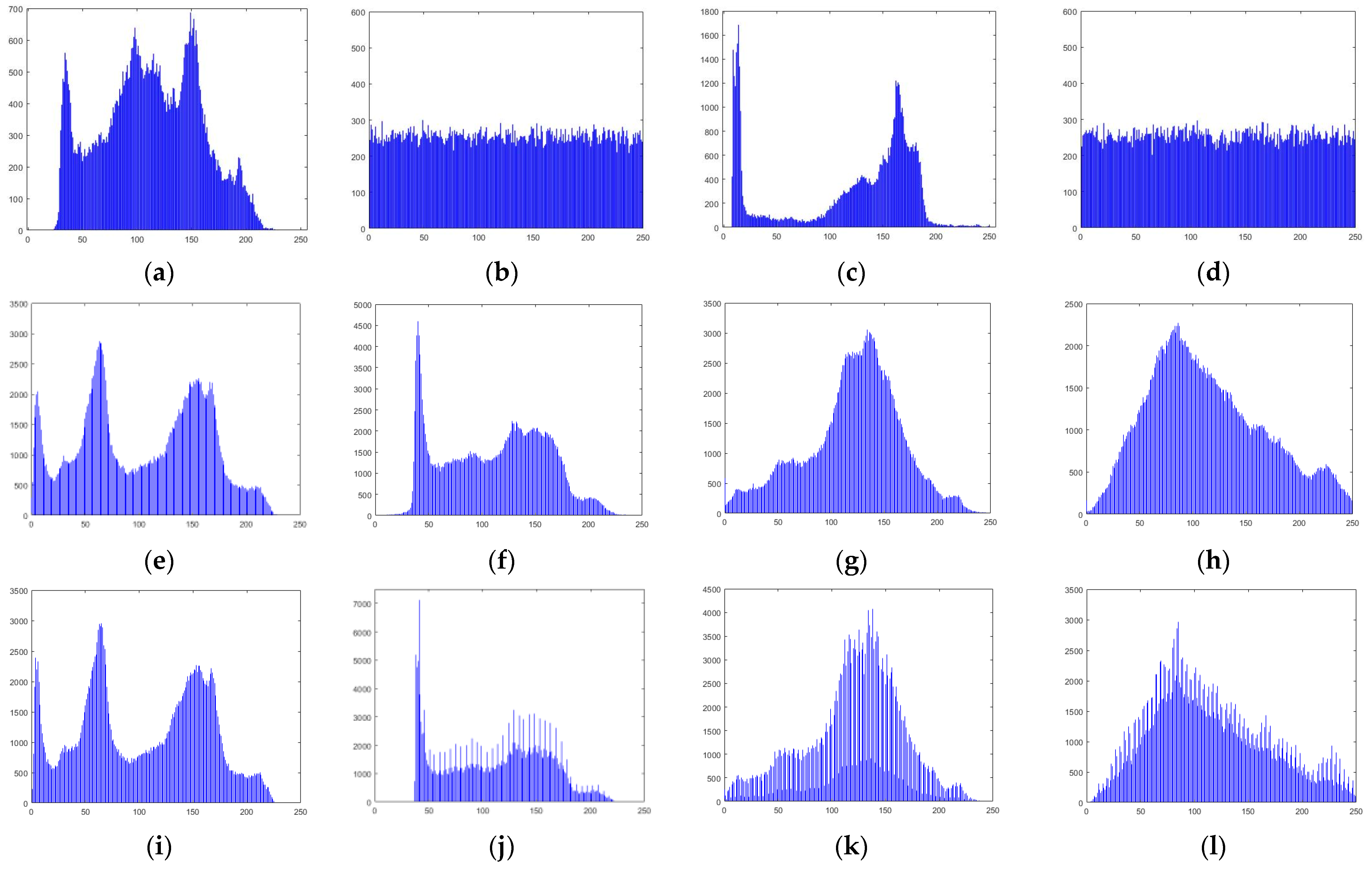
5.2.2. Histogram Analysis
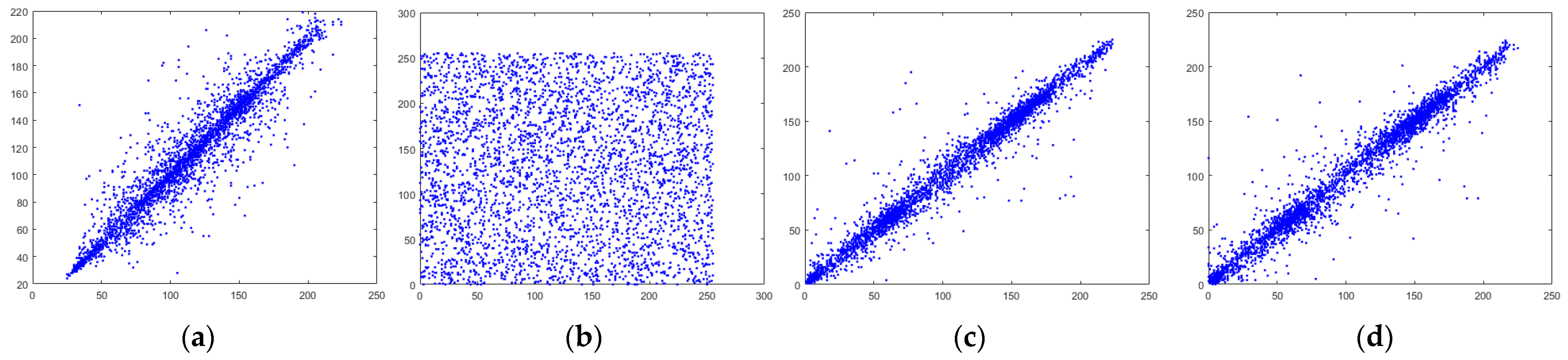
5.2.3. Correlation Analysis
5.3. Various Attacks
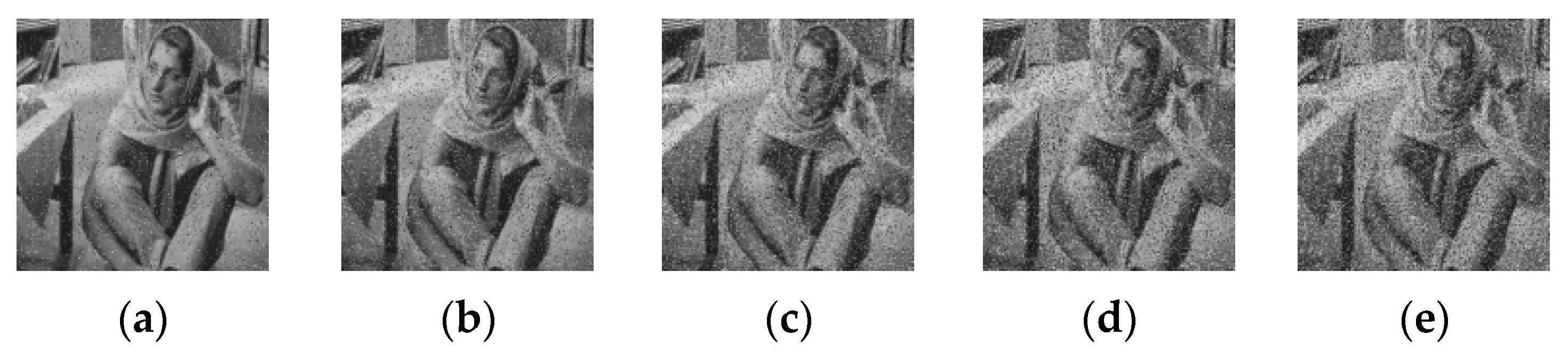
5.3.1. Noise Attack
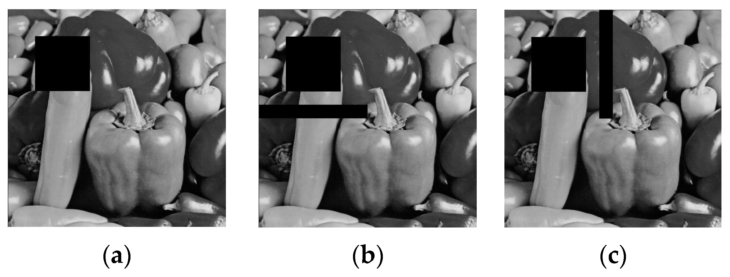
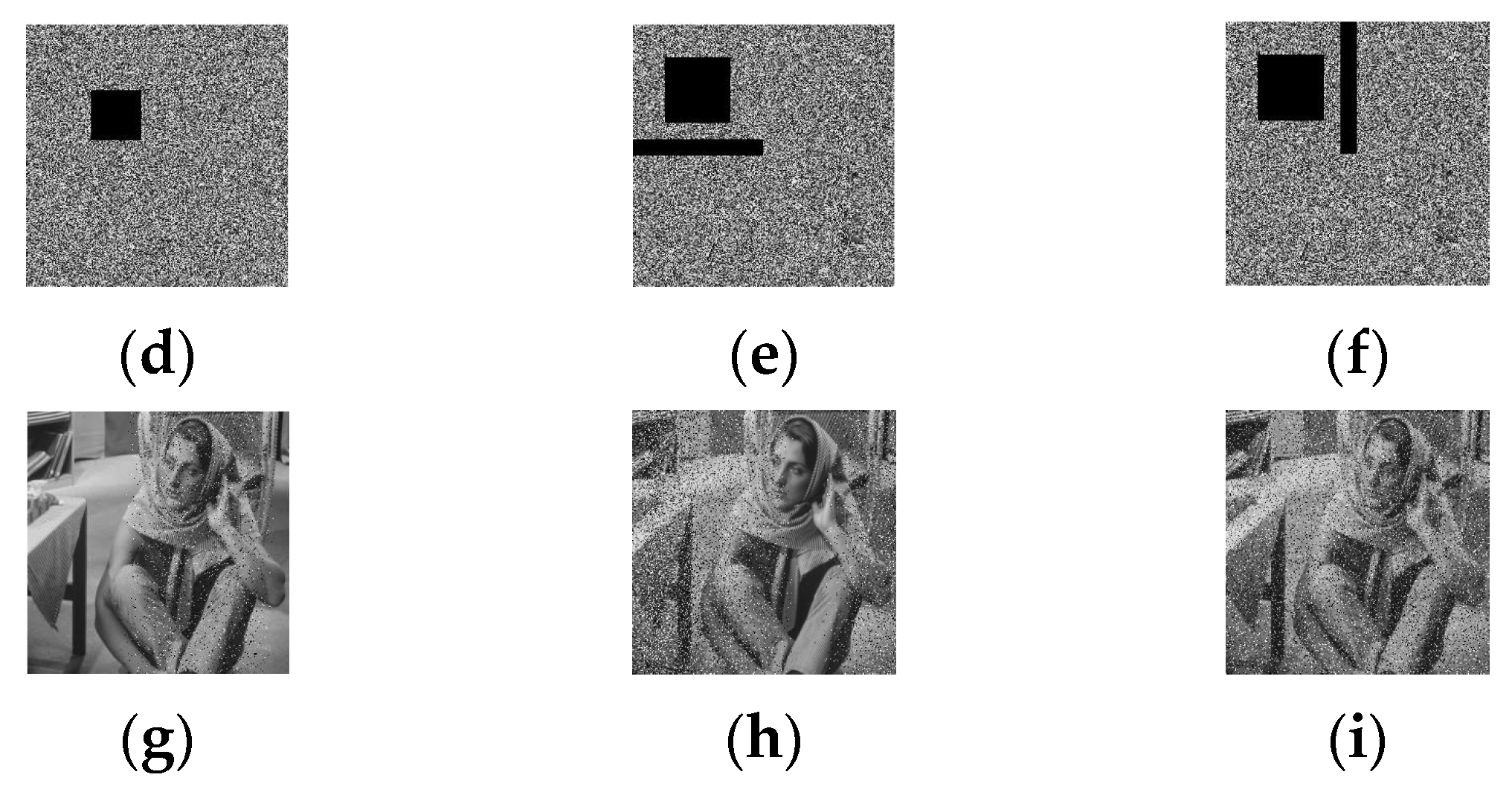
5.3.2. Cropping Attack
5.3.3. Differential Attack
5.3.4. Chosen-Plain Attack
5.4. Comparison with Existing Schemes
6. Conclusions
Author Contributions
Funding
Data Availability Statement
Conflicts of Interest
References
- Chua, L.O. Memristor-The missing circuit element. IEEE Trans. Circuit Theory 1971, 18, 159–182. [Google Scholar] [CrossRef]
- Strukov, D.B.; Snider, G.S.; Stewart, D.R.; Williams, R.S. The missing memristor found. Nature 2008, 453, 80–83. [Google Scholar] [CrossRef]
- Zhong, Y.; Tang, J.; Li, X.; Gao, B.; Qian, H.; Wu, H. Dynamic memristor-based reservoir computing for high-efficiency temporal signal processing. Nat. Commun. 2021, 12, 408. [Google Scholar] [CrossRef]
- Gul, F. Addressing the sneak-path problem in crossbar RRAM devices using memristor-based one schottky diode-one resistor array. Results Phys. 2019, 12, 1091–1096. [Google Scholar] [CrossRef]
- Bao, H.; Zhu, D.; Liu, W.; Xu, Q.; Chen, M.; Bao, B. Memristor synapse-based morris-lecar model: Bifurcation analyses and FPGA-based validations for periodic and chaotic bursting/spiking firings. Int. J. Bifurc. Chaos 2020, 30, 2050045. [Google Scholar] [CrossRef]
- Zhang, S.; Zheng, J.; Wang, X.; Zeng, Z.; He, S. Initial offset boosting coexisting attractors in memristive multi-double-scroll hopfield neural network. Nonlinear Dyn. 2020, 102, 2821–2841. [Google Scholar] [CrossRef]
- Zhou, P.; Yao, Z.; Ma, J.; Zhu, Z. A piezoelectric sensing neuron and resonance synchronization between auditory neurons under stimulus. Chaos Solit. Fract. 2021, 145, 110751. [Google Scholar] [CrossRef]
- Wu, X.; He, S.; Tan, W.; Wang, H. From Memristor-Modeled Jerk System to the Nonlinear Systems with Memristor. Symmetry 2022, 14, 659. [Google Scholar] [CrossRef]
- Lei, T.; Zhou, Y.; Fu, H.; Huang, L.; Zang, H. Multistability Dynamics Analysis and Digital Circuit Implementation of Entanglement-Chaos Symmetrical Memristive System. Symmetry 2022, 14, 2586. [Google Scholar] [CrossRef]
- Yang, B.; Wang, Z.; Tian, H.; Liu, J. Symplectic Dynamics and Simultaneous Resonance Analysis of Memristor Circuit Based on Its van der Pol Oscillator. Symmetry 2022, 14, 1251. [Google Scholar] [CrossRef]
- Dai, W.; Xu, X.; Song, X.; Li, G. Audio Encryption Algorithm Based on Chen Memristor Chaotic System. Symmetry 2022, 14, 17. [Google Scholar] [CrossRef]
- Rajagopal, K.; Kacar, S.; Wei, Z.; Duraisamy, P.; Kifle, T.; Karthikeyan, A. Dynamical investigation and chaotic associated behaviors of memristor chua’s circuit with a non-ideal voltage-controlled memristor and its application to voice encryption. AEU-Int. J. Electron. Commun. 2019, 107, 183–191. [Google Scholar] [CrossRef]
- Chen, J.; Yan, D.-W.; Duan, S.-K.; Wang, L.-D. Memristor-based hyper-chaotic circuit for image encryption. Chin. Phys. B 2020, 29, 110504. [Google Scholar] [CrossRef]
- Zhu, L.; Jiang, D.; Ni, J.; Wang, X.; Rong, X.; Ahmad, M. A visually secure image encryption scheme using adaptive thresholding sparsification compression sensing model and newly-designed memristive chaotic map. Inf. Sci. 2022, 607, 1001–1022. [Google Scholar] [CrossRef]
- Tsafack, N.; Iliyasu, A.M.; De Dieu, N.J.; Zeric, N.T.; Kengne, J.; Abd-El-Atty, B.; Belazi, A.; Abd EL-Latif, A.S. A memristive RLC oscillator dynamics applied to image encryption. J. Info. Sec. App. 2021, 61, 102944. [Google Scholar] [CrossRef]
- Chua, L.O. Local activity is the origin of complexity. Int. J. Bifur. Chaos 2005, 15, 3435–13456. [Google Scholar] [CrossRef]
- Mannan, Z.I.; Choi, H.; Kim, H. Chua corsage memristor oscillator via Hopf bifurcation. Int. J. Bifur. Chaos. 2016, 26, 1630009. [Google Scholar] [CrossRef]
- Chua, L.O. If it’s pinched it’s a memristor. Semicond. Sci. Technol. 2014, 29, 104001. [Google Scholar] [CrossRef]
- Williams, R.S.; Pickett, M.D. The Art and Science of Constructing a Memristor Model: Memristors and Memristive Systems; Springer: New York, NY, USA, 2013; pp. 93–104. [Google Scholar]
- Messaris, I.; Brown, T.D.; Demirkol, A.S.; Ascoli, A.; Al Chawa, M.M.; Williams, R.S.; Tetzlaff, R.; Chua, L.O. NbO2-Mott memristor: A circuit-theoretic investigation. IEEE Trans. Circuits Syst. I Regul. Pap. 2021, 68, 4979–4992. [Google Scholar] [CrossRef]
- Mannan, Z.I.; Choi, H.; Rajamani, V.; Kim, H.; Chua, L. Chua corsage memristor: Phase portraits, basin of attraction, and coexisting pinched hysteresis loops. Int. J. Bifur. Chaos 2017, 27, 1730011. [Google Scholar] [CrossRef]
- Mannan, Z.I.; Choi, H.; Rajamani, V. Oscillation with 4-lobe Chua corsage memristor. IEEE Circuits Syst. Mag. 2018, 18, 14–27. [Google Scholar] [CrossRef]
- Mannan, Z.I.; Yang, C.; Adhikari, S.P.; Kim, H. Exact analysis and physical realization of the 6-lobe Chua corsage memristor. Complexity 2018, 2018, 1–12. [Google Scholar] [CrossRef]
- Dong, Y.; Wang, G.; Chen, G.; Shen, Y.; Ying, J. A bistable nonvolatile locally-active memristor and its complex dynamics. Commun. Nonlinear Sci. 2020, 84, 105203. [Google Scholar] [CrossRef]
- Tan, Y.; Wang, C. A simple locally active memristor and its application in HR neurons. Chaos 2020, 30, 053118. [Google Scholar] [CrossRef]
- Xie, W.; Wang, C.; Lin, H. A fractional-order multistable locally active memristor and its chaotic system with transient transition, state jump. Nonlinear Dyn. 2021, 104, 4523–4541. [Google Scholar] [CrossRef]
- Ding, D.; Xiao, H.; Yang, Z.; Luo, H.; Hu, Y.; Zhang, X.; Liu, Y. Coexisting multi-stability of Hopfield neural network based on coupled fractional-order locally active memristor and its application in image encryption. Nonlinear Dyn. 2022, 108, 4433–4458. [Google Scholar] [CrossRef]
- Yang, Z.-L.; Liang, D.; Ding, D.-W.; Hu, Y.-B.; Li, H. Transient transition behaviors of fractional-order simplest chaotic circuit with bi-stable locally-active memristor and its ARM-based implementation. Chin. Phy. B. 2021, 30, 120515. [Google Scholar] [CrossRef]
- Bao, L.; Zhou, Y. Image encryption: Generating visually meaningful encrypted images. Info. Sci. 2015, 324, 197–207. [Google Scholar] [CrossRef]
- Chai, X.; Gan, Z.; Chen, Y.; Zhang, Y. A visually secure image encryption scheme based on compressive sensing. Signal Process. 2017, 134, 35–51. [Google Scholar] [CrossRef]
- Wang, H.; Xiao, D.; Li, M.; Xiang, Y.; Li, X. A visually secure image encryption scheme based on parallel compressive sensing. Signal Process. 2019, 155, 218–232. [Google Scholar] [CrossRef]
- Ping, P.; Yang, X.; Zhang, X.; Mao, Y.; Khalid, H. Generating visually secure encrypted images by partial block pairing-substitution and semi-tensor product compressed sensing. Digit. Signal Process. 2022, 120, 103263. [Google Scholar] [CrossRef]
- Li, R.H.; Dong, E.Z.; Tong, J.G. A Novel Multiscroll Memristive Hopfield Neural Network. Int. J. Bifur. Chaos. 2022, 32, 2250130. [Google Scholar] [CrossRef]
- Ying, J.; Liang, Y.; Wang, J.; Dong, Y.; Wang, G.; Gu, M. A tristable locally-active memristor and its complex dynamics. Chaos Solitons Fractals 2022, 160, 112241. [Google Scholar] [CrossRef]
- Carpinteri, A.; Mainardi, F. Fractals and Fractional Calculus in Continuum Mechanics; International Centre for Mechanical Sciences; Springer: Berlin/Heidelberg, Germany, 1997; Volume 378. [Google Scholar]
- Bremen, H.F.V.; Udwadia, F.E.; Proskurowski, W. An efficient QR based method for the computation of Lyapunov exponents. Physica D 1997, 101, 1–16. [Google Scholar] [CrossRef]
- Shen, E.H.; Cai, Z.J.; Gu, F.J. Mathematical foundation of a new complexity measure. Appl. Math. Mech. 2005, 26, 1188–1196. [Google Scholar]
- Erkan, U.; Toktas, A.; Enginoğlu, S.; Akbacak, E.; Thanh, D.N.H. An image encryption scheme based on chaotic logarithmic map and key generation using deep CNN. Multimed. Tools Appl. 2022, 81, 7365–7391. [Google Scholar] [CrossRef]
- Wang, Z.; Bovik, A.; Sheikh, H.; Simoncelli, E. Image quality assessment: From error visibility to structural similarity. IEEE Trans. Image Process. 2004, 13, 600–612. [Google Scholar] [CrossRef]
- Wang, X.Y.; Liu, C.; Jiang, D.H. Visually meaningful image encryption scheme based on new-designed chaotic map and random scrambling diffusion strategy. Chaos Solitons Fractals 2022, 164, 112625. [Google Scholar] [CrossRef]
- Zhu, L.; Song, H.; Zhang, X.; Yan, M.; Zhang, T.; Wang, X.; Xu, J. A robust meaningful image encryption scheme based on block compressive sensing and SVD embedding. Signal Process. 2020, 175, 107629. [Google Scholar] [CrossRef]


| Memristor Models | Number of Parameters | Number of Equilibrium Points |
|---|---|---|
| Ref. [17] | 1 | 3 |
| Ref. [25] | 1 | 3 |
| Ref. [33] | 2 | infinite |
| Ref. [34] | 1 | 5 |
| Ours | 7 | 5 |
| Rule | 1 | 2 | 3 | 4 | 5 | 6 | 7 | 8 |
|---|---|---|---|---|---|---|---|---|
| 00 | A | C | C | A | G | T | T | G |
| 01 | C | T | A | G | A | G | C | T |
| 10 | G | A | T | C | T | C | G | A |
| 11 | T | G | G | T | C | A | A | C |
| ⊙ | A | G | C | T |
|---|---|---|---|---|
| A | T | C | G | A |
| G | C | T | A | G |
| C | G | A | T | C |
| T | A | G | C | T |
| Plain Image | Carrier Image | p-r | p-r | c-v | c-v |
|---|---|---|---|---|---|
| Barbara | Peppers | 37.9526 | 0.9523 | 43.9256 | 0.9962 |
| Cameraman | Pirate | 38.8541 | 0.9567 | 43.2873 | 0.9952 |
| Circuit | Living room | 39.6512 | 0.9612 | 43.9638 | 0.9937 |
| House | Walk bridge | 39.0246 | 0.9528 | 43.4846 | 0.9990 |
| Average | 38.8706 | 0.95575 | 43.6653 | 0.9960 |
| Item | Barbara | Cameraman | Circuit | House | Average | Ref. [40] |
|---|---|---|---|---|---|---|
| (%) | 99.63 | 99.57 | 99.69 | 99.48 | 99.592 | 99.59 |
| (%) | 33.69 | 33.58 | 33.62 | 33.63 | 33.63 | 33.5 |
| Noise Type | Attack Intensity | PSNR | |||
|---|---|---|---|---|---|
| Ref. [14] | Ref. [31] | Ref. [41] | Ours | ||
| SPN | 0.0001 | 33.44 | 31.56 | 28.18 | 28.01 |
| 0.0003 | 33.26 | 30.22 | 28.18 | 27.77 | |
| 0.0005 | 33.02 | 30.02 | 28.17 | 27.58 | |
| Cropping | 24.92 | 27.21 | 30.18 | 30.35 | |
| 20.13 | 23.96 | 29.01 | 30.10 |
| Algorithm | Encryption | Embedding | Extraction | Reconstruction |
|---|---|---|---|---|
| Ref. [41] | 0.1262 | 0.1995 | 0.0833 | 0.4374 |
| ours | 0.1352 | 0.1024 | 0.0811 | 0.1578 |
Disclaimer/Publisher’s Note: The statements, opinions and data contained in all publications are solely those of the individual author(s) and contributor(s) and not of MDPI and/or the editor(s). MDPI and/or the editor(s) disclaim responsibility for any injury to people or property resulting from any ideas, methods, instructions or products referred to in the content. |
© 2023 by the authors. Licensee MDPI, Basel, Switzerland. This article is an open access article distributed under the terms and conditions of the Creative Commons Attribution (CC BY) license (https://creativecommons.org/licenses/by/4.0/).
Share and Cite
Wu, Y.; Wang, D.; Zhang, T.; Zhang, J.; Zhou, J. A Novel Fractional-Order Memristive Chaotic Circuit with Coexisting Double-Layout Four-Scroll Attractors and Its Application in Visually Meaningful Image Encryption. Symmetry 2023, 15, 1398. https://doi.org/10.3390/sym15071398
Wu Y, Wang D, Zhang T, Zhang J, Zhou J. A Novel Fractional-Order Memristive Chaotic Circuit with Coexisting Double-Layout Four-Scroll Attractors and Its Application in Visually Meaningful Image Encryption. Symmetry. 2023; 15(7):1398. https://doi.org/10.3390/sym15071398
Chicago/Turabian StyleWu, Yuebo, Duansong Wang, Tan Zhang, Jinzhong Zhang, and Jian Zhou. 2023. "A Novel Fractional-Order Memristive Chaotic Circuit with Coexisting Double-Layout Four-Scroll Attractors and Its Application in Visually Meaningful Image Encryption" Symmetry 15, no. 7: 1398. https://doi.org/10.3390/sym15071398
APA StyleWu, Y., Wang, D., Zhang, T., Zhang, J., & Zhou, J. (2023). A Novel Fractional-Order Memristive Chaotic Circuit with Coexisting Double-Layout Four-Scroll Attractors and Its Application in Visually Meaningful Image Encryption. Symmetry, 15(7), 1398. https://doi.org/10.3390/sym15071398