Abstract
Networks offer a compact representation of complex systems such as social, communication, and biological systems. Traditional network models are often inadequate to capture the diverse nature of contemporary networks, which may exhibit temporal variation and multiple types of interactions between entities. Multilayer networks (MLNs) provide a more comprehensive representation by allowing interactions between nodes to be represented by different types of links, each reflecting a distinct type of interaction. Community detection reveals meaningful structure and provides a better understanding of the overall functioning of networks. Current approaches to multilayer community detection are either limited to community detection over the aggregated network or are extensions of single-layer community detection methods with simplifying assumptions such as a common community structure across layers. Moreover, most of the existing methods are limited to multiplex networks with no inter-layer edges. In this paper, we introduce a spectral-clustering-based community detection method for two-layer MLNs. The problem of detecting the community structure is formulated as an optimization problem where the normalized cut for each layer is minimized simultaneously with the normalized cut for the bipartite network along with regularization terms that ensure the consistency of the within- and across-layer community structures. The proposed method is evaluated on both synthetic and real networks and compared to state-of-the-art methods. MLNs. The problem of detecting the community structure is formulated as an optimization problem where the normalized cut for each layer is minimized simultaneously with the normalized cut for the bipartite network along with regularization terms that ensure the consistency of the intra- and inter-layer community structures. The proposed method is evaluated on both synthetic and real networks and compared to state-of-the-art methods.
1. Introduction
Networks provide a compact representation of the internal structure of complex systems consisting of agents that interact with each other. Some example application areas include social sciences, engineering systems, and biological systems [1,2]. A core task in network analysis is community detection, which identifies the partition of the node set such that within-community connections are denser than between-community connections.
While different methods have been proposed to detect the community structure of simple (single-layer) graphs, in many contemporary applications, a pair of nodes may interact through multiple types of links yielding multilayer networks. In MLNs, each type of link represents a unique type of interaction. These links can be separated into different layers, enabling the same group of nodes to be connected in multiple ways [3]. The layers in a multilayer network can represent various attributes or features of a complex system. For instance, they can be temporal snapshots of the same network at different time intervals, or they can correspond to different types of connections in social networks, e.g., friendship, collaboration, or family relationships, different types of units in military tactical networks, e.g., infantry, vehicles, or airborne units [4], or transportation networks, where nodes representing different locations can be linked through various modes of transportation, including roads, railways, and air routes. Multilayer networks can further be categorized based on the homogeneity of the nodes and complexity of topological structure as (i) multiplex networks that exhibit homogeneity in terms of the entities they comprise, with each layer consisting of the same set of entities of the same type where the inter-layer edges are implicit and not shown; (ii) heterogeneous multilayer networks by the possibility of having different sets and types of entities for each layer and the relationships between entities across layers are explicitly represented by inter-layer edges.
Current approaches to multilayer community detection are either limited to community detection over the aggregated network or are extensions of single-layer community detection methods with simplifying assumptions such as a common community structure across layers. Moreover, they are mostly limited to multiplex networks with no inter-layer edges.
In this paper, we extend the notion of spectral clustering from single-layer networks to two-layer networks with inter-layer edges. In particular, we model the two-layer network as the union of two single-layer networks and a bipartite network that is represented through its symmetric rows’ and columns’ adjacency matrices. Next, we express the cost functions corresponding to minimizing the normalized cut for each of the layers as well as the inter-layer adjacency matrix in its relaxed form similar to spectral clustering. In order to ensure the consistency of the communities across layers, we regularize the resulting cost function by a projection distance metric that quantifies the consistency of the low-rank embeddings of the networks across layers. The resulting optimization problem is solved through an alternating maximization scheme.
2. Related Work
Community detection methods for multilayer networks can be broadly categorized into three classes: flattening methods, aggregation methods, and direct methods. Flattening methods convert the multilayer network into a single-layer network by collapsing the layers and then apply traditional community detection algorithms. This approach ignores the information present in the multiple layers, which can lead to loss of important features and inaccuracies in the community structure [5]. Aggregation methods detect the community structure for each layer separately and then merge the results into a single structure. This method requires a merging strategy to combine the community structures from each layer, which can be challenging and subjective. Additionally, it may fail to capture the inter-layer dependencies and correlations between the layers [6]. Direct methods work directly on the multilayer network and optimize community-quality assessment criteria such as modularity or normalized cut to identify the community structure. This approach accounts for the interactions between the layers and can reveal the inter-layer dependencies and correlations [7,8,9].
Some examples of the direct method include multilayer label propagation, random-walk-based methods, non-negative matrix factorization, modularity, and spectral-clustering-based methods. Label propagation algorithms (LPAs) propagate node attributes based on their neighbors’ behavior and exhibit linear complexity. Inspired by the traditional LPA, the authors of [10] presented a redefinition of the neighborhood in multilayer networks and proposed a multilayer LPA. Although this approach is efficient and can handle weighted and directed networks, the resulting partition is highly dependent on the threshold parameter and the density of the network dataset. Moreover, this method is only suitable for multiplex networks. Kuncheva et al. [9] proposed locally adaptive random transitions (LARTs), which are designed to detect communities that are shared by some or all layers in multiplex networks. More recently, matrix and tensor factorization methods have been proposed for multilayer community detection. Among these, non-negative matrix factorization (NMF)-based methods that extract low-dimensional feature representations for each layer, where collective factorization is then used to fuse them into a common representation [11]. In [12], a semi-supervised joint non-negative matrix factorization (S2-jNMF) algorithm is proposed for community detection in multiplex networks, aiming to detect a common structure across layers. However, all of these methods are restricted to multiplex networks, where inter-layer edges are only allowed between each node and its corresponding replicas across different layers.
More recently, community detection methods that consider fully connected MLNs, MLNs with inter-relations, have been proposed [13]. The authors of [14,15] propose to extend the modularity function and its solution to account for MLNs with inter-layer relations. Similarly, [16] propose a normalized cut extension to MLNs by creating a block Laplacian matrix, where each block corresponds to a specific layer. The community structure is then obtained through standard spectral clustering on this block Laplacian matrix. However, the selection of the parameter is crucial to ensuring the community structure consistency across the layers in this method. Another commonly employed technique that incorporates the concept of network dynamics, specifically diffusion, is Infomap [17]. This method optimizes the map equation, which leverages the information–theoretic relationship between reducing network dimensionality and detecting network communities. However, in the case of noisy networks, the efficiency of the diffusion process, i.e., information propagation, may be compromised, leading to suboptimal clustering performance [18].
3. Background
3.1. Graph Theory
Single-layer network: A single-layer network or a simple graph models the interactions between entities in network science. A single-layer network can be defined as , where is the set of nodes, is the set of edges, and is the symmetric adjacency matrix, with being the number of nodes.
Bipartite network: A bipartite network or graph is a graph that can be partitioned into two sets of vertices where all edges connect vertices from one set to vertices in the other set. Formally, a bipartite graph is defined as , where , are the disjoint sets of vertices and the set of edges that connects a vertex in to a vertex in . denotes the symmetric adjacency matrix of the bipartite network, where and refer to the size of the two disjoint sets. The adjacency matrix of the bipartite graph can be defined as follows:
where describes the relationships between and .
Two-layer network: A two-layer network is a type of multilayer network that consists of two layers or graphs, where each layer represents a different type of relationship or interaction between nodes. A two-layer network, , can be formally defined as the set of two single-layer graphs, and , and a bipartite graph, , such that with , , and . and are known as within- or intra-layer graphs, whereas refers to the across- or inter-layer graph.
Supra-adjacency matrix: A supra-adjacency matrix is a symmetric matrix that represents both the intra- and inter-layer connections in a multilayer network. A supra-adjacency matrix of a two-layer MLN, , where can be constructed from the intra- and inter-layer adjacency matrices as follows:
where , , and .
3.2. Graph Cut Problem and Spectral Clustering
Graph minimum cut (mincut) is a problem in graph theory that involves partitioning a graph into multiple partitions or disjoint sets of nodes such that the number of edges between these sets is minimized. The mincut problem is NP-hard. However, there are efficient algorithms to approximate the mincut, such as spectral clustering. Spectral clustering relies on the spectral properties (eigenvalues and eigenvectors) of the symmetric graph Laplacian matrix or normalized adjacency matrix. In particular, spectral clustering uses these eigenvalues and eigenvectors to embed the nodes of the graph into a lower-dimensional space. The nodes can be then clustered using standard k-means in this lower-dimensional space.
Given a single-layer graph with a symmetric adjacency matrix, , spectral clustering solves the following trace maximization problem [19,20]:
where “” and “⊤” refer to the trace and transpose operators, respectively. is the normalized version of the adjacency matrix, where D is the degree matrix with . Spectral clustering uses the spectrum (eigenvalues) of the normalized adjacency matrix to partition the nodes into clusters. In particular, the eigenvectors corresponding to the largest k eigenvalues are used to embed the nodes in a low-dimensional space, where the matrix U is constructed by arranging these eigenvectors as its columns. The final structure is then determined by applying classical k-means to the rows of the matrix U [19]. The number of the eigenvectors, k, corresponds to the number of communities in the network.
3.3. Spectral Co-Clustering in Bipartite Networks
Bipartite spectral co-clustering is a technique for simultaneously clustering both rows and columns of a bipartite network [21,22]. The problem can be formulated as a trace maximization problem as follows:
where , , with , and . According to the Ky Fan theorem, the global optimum solution of Equation (4) is the matrix Z containing k eigenvectors that correspond to the largest eigenvalues of .
A more computationally efficient solution [21] to solve Equation (4) is to compute and as the matrices containing the left and right singular vectors that correspond to the largest k singular values of the matrix , respectively.
Another approach to solve Equation (4) is by first computing the symmetric rows and columns adjacency matrices, and , and then solving two trace maximization problems, simultaneously, as follows [22]:
where and can be computed separately as the eigenvectors’ matrices related to the largest k eigenvalues of and , respectively.
3.4. Projection Distance between Subspaces
The projection distance between subspaces measures the distance between two subspaces of a vector space. In particular, it quantifies the distance between the orthogonal projections of a vector onto each of the two subspaces. Let and be two subspaces and their corresponding orthonormal basis sets are and , respectively. The projection distance can be determined by the principal angles between the two subspaces. Let denote the ith principal angle between the two subspaces; then, the projection distance is defined as [23]:
4. Community Detection in Multilayer Networks: A Unified Spectral Clustering Approach (ML-USCL)
4.1. Problem Formulation
Given a two-layer network, in order to determine a community, , two subsets of vertices are defined: (i) within-layer community subset, , with and , where , and (ii) across-layer community subset, with and . A community can then be defined as , where it may include vertices from one or more layers in the network. In particular, defines either a within-layer community when or an across-layer community when .
In this paper, the objective is to partition a two-layer network into K disjoint communities. The goal is to find the low-rank embeddings of each layer to maximize the separability between communities while ensuring that these low-rank embeddings are consistent with the partitioning of the inter-layer graph. This objective is achieved by exploiting previous work in spectral clustering of single-layer networks and spectral co-clustering of bipartite networks. More precisely, intra-and inter-layer graphs are modeled as single-layer and bipartite graphs, respectively. The intra-layer graph encodes the interactions between nodes within the same layer, whereas the inter-layer graph encodes the interactions between nodes from both layers.
The proposed objective function can be expressed mathematically as:
The proposed objective function is formulated such that the first two terms refer to the spectral clustering problem for Layers 1 and 2, respectively, where and are the symmetric normalized intra-layer adjacency matrices. The third and fourth terms refer to the bipartite spectral clustering problem. The last two terms define the spectral embedding similarity between the left and right subspaces of and the low-rank subspaces of and , respectively [24,25,26]. In particular, maximizing these two terms minimizes the projection subspace distance between and , ensuring the consistency between the intra- and inter-layer partitions. and refer to the number of within-layer communities in Layers 1 and 2, respectively, whereas k refers to the number of across-layer communities. and are the regularization parameters.
4.2. Problem Solution
4.2.1. Initializing the Intra- and Inter-Layer Basis Matrices
Intra-layer basis matrices, and , are initialized using Equation (3). The number of communities, and , in each one of the layers is determined initially by the asymptotical surprise (AS) metric [27]. In particular, the AS metric is calculated for a range of possible community numbers, and the initial number of intra-communities is set to the number that achieves the maximum value of the AS metric. On the other hand, inter-layer basis matrices, and , are initialized using Equation (5), where . The steps of initializing the basis matrices are oultined in Algorithm 1.
| Algorithm 1 Initializing the intra- and inter-layer basis matrices |
| Input:, , , maximum number of communities (). |
| Output: Initial (, , and ), , , k |
|
4.2.2. Finding the Basis Matrices
As solving for the different variables in the proposed objective function jointly is not feasible, alternating maximization can be adopted to compute the variables, iteratively. Alternating maximization is a commonly used approach for solving optimization problems that involve multiple variables or constraints. In particular, the technique involves fixing one set of variables and computing the other set, alternating between the two until convergence [28,29].
The solution to the proposed problem in Equation (7) can be found using an alternating maximization scheme as follows:
- Update : By considering only the terms that contain , we obtainwhere is the modified normalized adjacency matrix representing Layer 1. The solution to this problem is similar to the classic spectral clustering formulation. In particular, the matrix is computed through eigen decomposition (ED) of , where it consists of the eigenvectors that are associated with the largest eigenvalues of .
- Update : By considering only the terms that contain we obtain,where is the modified normalized adjacency matrix representing Layer 2. Similar to , contains eigenvectors associated with the largest eigenvalues of .
- Update : By considering only the terms that contain , we obtainwhere is referred to as the modified normalized adjacency matrix that represents the rows of the inter-layer graph and can be computed also through eigendecomposition and it comprises the eigenvectors corresponding to the k largest eigenvalues of .
- Update : By keeping all the terms that include only , we obtainwhere indicates the modified normalized adjacency matrix that represents the columns of the inter-layer graph, and represents the eigenvector matrix that corresponds to the k largest eigenvalues of .
As it can be seen from the update steps outlined above, each of the basis matrices is found jointly using both intra- and inter-layer adjacency information. In particular, is the subspace corresponding to both its corresponding adjacency matrix and the Gram matrix defined by , i.e., . Similar arguments can be made for the other basis matrices showing that they are learned to optimize the span for both within- and between-layer connectivity. After the basis matrices are computed, a set of intra- and inter-layer communities are determined by applying k-means to , , and . The final community structure of the network is then determined by following the steps explained in Section 4.3.
4.3. Determining the Final Community Structure of the Network
After estimating a set of within- and across-layer communities, we evaluate their quality as follows:
- The quality or strength of each within- and across-layer community is measured using the communitude metric [30,31] in terms of the supra-adjacency matrix as:where is the sum of internal edges in a community, i.e., edges between the nodes in the same community or “within-community” edges; is the sum of external edges in a community, i.e., edges that connect nodes belonging to different communities or “between-community” edges; and refers to the sum of all edges in the supra-adjacency. In fact, this quality function can be seen as an adapted form of the Z-score function, where it is normalized by the standard deviation of the fraction of the number of edges within the subgraph. The upper bound of the communitude metric is 1.
- To identify the most significant communities in a network, the communities are ranked in descending order depending on their communitude values. Every node in the proposed ML-USCL is allowed to join one community, within- or across-layer community. In particular, the communitude values of both the within- or across-layer communities are compared; then, the community that scores a higher value is selected.
- The final community structure of the two-layer MLN is then considered as the set of K communities, , that scores the largest communitude values.
The steps of the developed algorithm are summarized in Algorithm 2.
| Algorithm 2 Detecting Community Structure in Multilayer networks: Unified Spectral Clustering (ML-USCL) |
| Input: , , , , |
| Output: Within- and across-layer communities. |
|
4.4. Computational Complexity of ML-USCL
The order of complexity of the proposed ML-USCL depends on the specific implementation of the algorithm and the size of the input network. The main steps involved in the proposed ML-USCL include initializing the basis matrices, updating the basis matrices by performing eigenvalue decomposition, and applying k-means to get the within- and across-layer communities.
Let be the number of nodes in the mth layer; then, initializing each one of the basis matrices requires eigenvalue decomposition of the intra- and inter-layer adjacency matrices, which has a complexity of . During the initialization step, the number of communities in each of the intra-layer graphs is determined by calculating the AS metric over a range of communities, . The AS calculation requires , where refers to the number of edges in the layer. For each iteration, the update of has a complexity of . Applying k-means to to get the clustering labels requires , where refers to the number iterations taken by the k-means.
Overall, the complexity of the proposed ML-USCL is dominated by the eigenvalue decomposition step. In particular, the order of complexity when full eigenvalue decomposition is calculated can be determined as , where refers to the total number of iterations. However, this computational complexity can be reduced to by computing the leading eigenvectors. Consequently, the order of complexity of the proposed ML-USCL can be considered as since the leading eigenvectors are computed in each iteration.
5. Results and Discussion
In this section, multiple experiments are conducted to evaluate the significance of the proposed approach. All experiments are performed on a standard Windows 10 Server with Intel (R) Core (TM) i7-9700 CPU @ 3.00GHz and 16GB RAM, MATLAB R2022b. The performance of the proposed ML-USCL is compared to other existing approaches, including block spectral clustering with inter-layer relations (BLSC), where as suggested by the approach [16], generalized Louvain (GenLov) [32], collective NMF approaches [11], including CSNMTF and CPNMF. The input to the BLSC, GenLov, and collective NMF is the two-layer network directly, supra-adjacency, and the multiplex version of the network, respectively. The number of communities is determined using the asymptotical surprise for BLSC and the collective NMF methods, while it is self-optimized in GenLov. The value of the maximum number of communities, , is determined based on the size of the network. For example, can be set to 20 for small networks and to 100 for large networks. The quality of the network’s final partition is evaluated using normalized mutual information (NMI) [33], adjusted Rand index (ARI) [34], and purity [35].
5.1. Simulated Networks
5.1.1. LFR Binary Simulated Networks
- LFR benchmark description: The Lancichinetti–Fortunato–Radicchi (LFR) benchmark [36,37] is a commonly used benchmark for evaluating the performance of community detection algorithms. In this experiment, the LFR benchmark is adopted to generate two-layer simulated networks, each with n nodes. The LFR benchmark uses a truncated power-law distribution to determine the community sizes. The parameters that control the community structure in the generated networks are (i) minimum degree, , (ii) maximum degree, , and (iii) mixing parameter, . The minimum and maximum values of the degree distribution ( and , respectively) are chosen such that the average degree of the network is equal to . Within-layer graphs are generated with and communities, whereas the across-layer graph is generated such that the ratio of the across-layer communities to the total number of communities is greater than or equal to , where . These selected communities are randomly combined with each other to create an across-layer community. The connection density within communities is set to and between communities to . The parameter controls the degree of inter-community connectivity, where a low value results in a strong community structure with few inter-community links, while a high value results in a weaker community structure with more inter-community links. On the other hand, controls the percent of the across-layer communities. As increases, the networks tend to have more across-layer communities.
- Experiment: In this experiment, two-layer unweighted networks with are created. The parameters of the generated networks are , , , and . To assess the efficacy of various algorithms in detecting community structure, a comparative analysis is carried out as the mixing parameter increases, i.e., the noise increases. Figure 1 shows a comparison between the different approaches in recovering the structure of two-layer LFR networks. Figure 1a–c reflect the performance of the different approaches when the two-layer network consists of within-layer communities only, i.e., . As it can be noticed from the figures, the proposed ML-USCL outperforms the other methods significantly over the different values of the mixing parameter, , with respect to all of the evaluation metrics. In Figure 1d–f, where , the two-layer networks comprises both intra- and inter-layer communities, the proposed ML-USCL exceeds the other algorithms in terms of the purity metric, and its performance is comparable to GenLov and BLSC with respect to the NMI and ARI metrics. Yet, the proposed ML-USCL performs better than both methods as the value of increases, which reflects its robustness. In Figure 1g–i, the networks consist of across-layer communities only. As illustrated in the figures, the proposed ML-USCL achieves higher scores of purity over the range of , whereas GenLov and BLSC achieve better performance in terms of NMI and ARI. This improvement in the performance of GenLov and BLSC compared to the networks with and is due to the fact that the networks consist of larger communities. However, the performance of both methods is inferior to ML-USCL for , which indicates that BLSC and GenLov are not robust to noise.
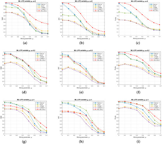 Figure 1. Comparison conducted among the various methods to evaluate their effectiveness in detecting the community structure. of LFR benchmark binary networks in terms of NMI, ARI, and purity with and variable mixing parameter : (a–c) ; (d–f) ; (g–i) .
5.1.2. Weighted Simulated Networks
- Weighted network description: The two-layer simulated weighted MLNs are generated from a truncated Gaussian distribution in the range of . The networks are generated based on the parameters (, ) and (, ), which refer to the mean and standard deviation of edge weights within and between communities, respectively. Several two-layer MLNs are generated by varying the ground-truth structure, including the number of communities (NOCs). Furthermore, a percentage of sparse noise () is randomly introduced into the networks to assess the algorithms’ ability to handle noise.
- Experiment: In this experiment, multilayer weighted networks (MLWNs) with 2 layers and 100 nodes per layer are generated. The parameters of the constructed MLWNs are reported in Table 1. Three different MLWNs are generated with different ground-truth communities and varying sparse noise levels, . The proposed ML-USCL is compared to the other algorithms, and the results are shown in Figure 2. It is evident from Figure 2 the superiority of ML-USCL compared to the other algorithms in weighted networks in terms of all metrics. Moreover, the proposed approach exhibits robustness to the addition of sparse noise, with the ability to accurately detect the community structure even as the percentage of added sparse noise, SPN%, increases.
 Table 1. Parameters of the simulated weighted two-layer MLNs.
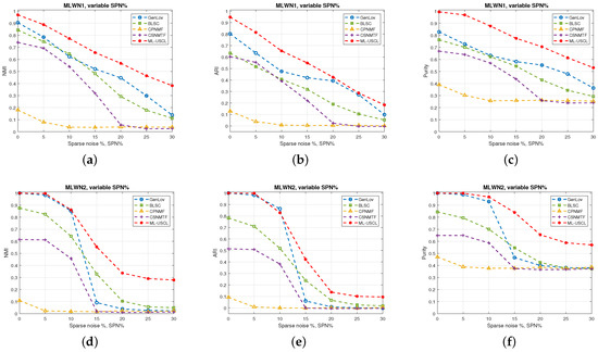
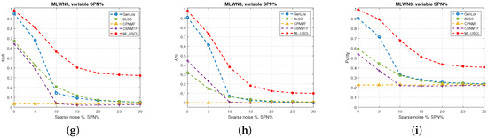 Figure 2. Comparison conducted among the various methods to evaluate their effectiveness in recovering the community structure of the multilayer weighted networks (MLWNs) from Table 1 in terms of NMI, ARI, and purity with different levels of added sparse noise percent (SPN%): (a–c) MLWN1; (d–f) MLWN2; (g–i) MLWN3.
5.2. Scalability Comparison
To evaluate the scalability of the proposed ML-USCL, we constructed a set of weighted multilayer networks with varying sizes. The network sizes ranged from 32 to 8192 on a logarithmic scale. For each network, the within- and between-community edges were randomly selected from a truncated Gaussian distribution within the range of using the following parameters: , , , , , , , , , , , and , where the superscripts refer to the within- and across-layer graphs. Each network consisted of two equal-sized communities: and in Layer 1, and and in Layer 2. The community structure of the multilayer network comprised , , and . The number of communities was specified as an input for all the algorithms. The run time of the different algorithms was measured as the network size varied, and the results are displayed in Figure 3. Figure 3 illustrates that the run time of the different methods exhibits a log-linear relationship as the number of nodes increases. Moreover, the proposed ML-USCL performs better than CSNMTF as the number of nodes grows, and it is comparable to BLSC and CPNMF. However, GenLov exhibits a faster run time compared to ML-USCL. The order of complexity of the different algorithms is given in Table 2. Nonetheless, as shown by the different experiments, the proposed algorithm maintains good performance compared to all other methods in terms of detecting an accurate community structure.
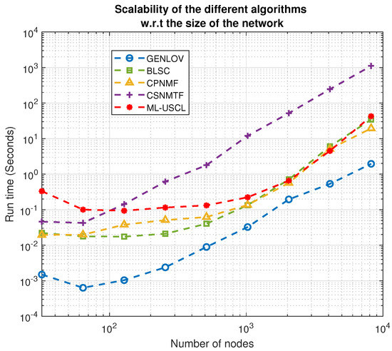
Figure 3.
Scalability comparison between the different methods.
Table 2.
Computational complexity of the different methods: M is the number of layers, n is the total number of nodes in the MLN, is the number of nodes in the mth layer, is the maximum number of iterations required by CSNMTF, is the maximum number of iterations required by CPNMF, is the maximum number of iterations required by ML-USCL, K is the number of communities in the MLN, and is the number of communities in the mth layer.
5.3. Regularization Parameters Selection
The proposed ML-USCL incorporates two regularization parameters, namely and . Both parameters penalize the similarity between the orthonormal subspaces within and across layers. The impact of these regularization parameters on the algorithm’s performance is investigated through experimental validation. We observed that the selection of and depends on the characteristics of the multilayer network under examination. If the network primarily consists of within-layer communities, smaller values of the regularization parameters are advised. Conversely, if the network comprises predominantly across-layer communities or both within- and across-layer communities, larger values of the parameters are recommended. In the proposed ML-USCL, we search for the best and jointly over a grid of [0.1–10].
5.4. Real-World Networks
To evaluate the effectiveness of the proposed method and compare it with other algorithms in identifying the community structure in real-world networks, four real-world networks are considered, as shown in Table 3. A brief description of these networks is given in the following section.
Table 3.
Description of the two-layer real networks.
5.4.1. Networks Description
- Lazega law-firm network (https://manliodedomenico.com/data.php) (accessed on 20 June 2023) [38] is a multilayer network that represents the interactions between 71 partners and associates in a corporate law partnership, where each layer corresponds to a specific type of interaction among the individuals. The intra-layer graphs capture co-work and advice relationships, while the inter-layer graph reflects friendship relationships. The dataset also includes seven attributes that can be used to evaluate the quality of the detected communities. In this study, the ground-truth community structure is determined based on the office location attribute, which could be either Boston, Hartford, or Providence.
- MIT Reality Mining (http://reality.media.mit.edu/download.php) (accessed on 20 June 2023) [39] network depicts various modes of mobile phone communication among 87 users, with edges indicating physical location, Bluetooth scans, and phone calls. The network (https://github.com/VGligorijevic/NF-CCE/tree/master/data/nets) (accessed on 20 June 2023) is constructed as a two-layer network, where the intra-layer graphs represent the physical location and Bluetooth scans, and the inter-layer graph represents phone call interactions. Further details on the construction of the network can be found in [40]. The ground-truth community structure in this network corresponds to the affiliations of the users.
- The C. Elegans network (https://manliodedomenico.com/data.php) (accessed on 20 June 2023) [8,41] is a multilayer network that depicts the synaptic junctions, including electric and chemical monadic and polyadic, between neurons in the C. Elegans nervous system. The network comprises 279 neurons and each neuron is grouped into different categories such as bodywall, mechanosensory, and head motor neurons. These categories can be considered as the ground-truth structure. In the constructed two-layer network, intra-layer edges denote the monadic and polyadic synaptic junctions among neurons, whereas inter-layer edges represent the electric junctions.
- Cora (https://people.cs.umass.edu/~mccallum/data.html) (accessed on 20 June 2023) data set is a subset of the Cora bibliographic data set. The Cora MLN consists of 292 nodes that refer to research papers. The intra-layer edges reflect the title and abstract similarities between the different research papers and the inter-layer edges model the citation relationships between them. The clusters in the network correspond to the research fields, namely data mining, natural language processing, and robotics.
- COIL20 (https://www.cs.columbia.edu/CAVE/software/softlib/) (accessed on 20 June 2023) is a data set comprising 1440 images obtained from the Columbia object image library where intra- and inter-layers represent different image features. Intra-layer graphs represent the local binary patterns (LBPs) and Gabor features, whereas inter-layer graphs represent the intensity feature. The data set consists of 20 communities, each referring to a group of related images.
- UCI (https://archive.ics.uci.edu/ml/datasets/Multiple+Features) (accessed on 20 June 2023) [42] consists of features extracted from handwritten digits (0–9) obtained from a collection of Dutch utility maps. The dataset contains a total of 2000 digit patterns, with 200 patterns per digit. These patterns are represented using different sets of features, including Fourier coefficients of the character shapes, profile correlations, and Karhunen–Loéve coefficients.
5.4.2. Experiments
The accuracy of the proposed ML-USCL in uncovering the community structure of the four real-world networks is evaluated and compared with other existing methods. The results are reported in Table 4. Based on the table, it is evident that the proposed ML-USCL for community detection in two-layer MLNs shows significant improvement over other algorithms. The evaluation of the community structure is performed individually for each layer and the proposed approach exhibits better performance than the other algorithms, as it achieves superior results in at least one quality metric in both layers. This indicates that the proposed approach is highly effective in identifying communities in MLNs. Moreover, the run time required for each one of the methods is presented in Table 5, where the proposed ML-USCL is faster than CSNMTF and CPNMF, comparable to BLSC and slower than GenLov. Nevertheless, ML-USCL exceeds the other algorithms in performance. These results suggest that the proposed approach can be a valuable tool in various applications that require the identification of communities in MLNs, such as social, biological, phone, and citation network analysis. Overall, the proposed approach has the potential to advance the field of community detection in MLNs and enable more accurate and efficient analysis of complex systems.
Table 4.
Community detection performance comparison for real-world multilayer networks.
Table 5.
Run time taken by the different methods for the real-world MLNs.
6. Conclusions
Community detection in multilayer networks is an active research area with various challenges and opportunities. The structure of multilayer networks provides additional information that can be used to enhance the accuracy and interpretability of community detection methods. In this article, a unified spectral-clustering-based community detection method for two-layer MLNs is introduced. The task of identifying the community structure in two-layer MLNs is expressed as an optimization problem, in which the normalized cut is minimized for each layer while also considering the normalized cut for the bipartite network. This optimization is performed concurrently with regularization terms that ensure the coherence of the community structures both within and across layers.
Multiple experiments have been conducted to evaluate the effectiveness of the proposed approach for community detection in two-layer unweighted and weighted simulated and real-world MLNs. These experiments demonstrate the efficiency and accuracy of the proposed ML-USCL in detecting the community structure in two-layer MLNs. In addition, ML-USCL is robust to noise compared to existing approaches. Finally, the ability to use the same objective function for both weighted and unweighted networks, while being robust to noise and outliers, makes the proposed method applicable to a wide range of MLNs.
For future work, we will focus on generalizing the proposed ML-USCL and addressing its limitations. In particular, the proposed approach will be extended to handle MLNs with more than two layers. The extension will be developed by first constructing a multidimensional array or tensor that represents the multilayer network and then applying tensor decomposition to reveal the underlying communities in the network. Finally, we would like to point out that the proposed approach in its current formulation can be adopted to detect the community structure in heterogeneous MLNs, i.e., nodes in the different layers refer to different objects. Future work will perform more experiments to validate the extension of the proposed ML-USCL in heterogeneous MLNs.
Author Contributions
Conceptualization, E.A.-s. and S.A.; methodology, E.A.-s. and S.A.; software, E.A.-s. and S.A.; validation, E.A.-s. and S.A.; formal analysis, E.A.-s. and S.A.; validation, E.A.-s. and S.A.; investigation, E.A.-s. and S.A.; resources, E.A.-s. and S.A.; data curation, E.A.-s. and S.A.; writing—original draft preparation, E.A.-s. and S.A.; writing—review and editing, E.A.-s. and S.A.; visualization, E.A.-s. and S.A.; supervision, E.A.-s. and S.A.; project administration, E.A.-s. and S.A.; funding acquisition, E.A.-s. and S.A. All authors have read and agreed to the published version of the manuscript.
Funding
This work was supported in part by the Jordan University of Science and Technology under Research Grant Number 20220277 and the National Science Foundation under CCF-2006800.
Institutional Review Board Statement
Not applicable.
Informed Consent Statement
Not applicable.
Data Availability Statement
Not applicable.
Acknowledgments
We would like to thank our colleague Abdullah Karaaslanli for providing us with the multilayer LFR network code.
Conflicts of Interest
The authors declare no conflict of interest.
References
- Boccaletti, S.; Latora, V.; Moreno, Y.; Chavez, M.; Hwang, D.U. Complex networks: Structure and dynamics. Phys. Rep. 2006, 424, 175–308. [Google Scholar] [CrossRef]
- Al-Sharoa, E.; Al-Khassaweneh, M.; Aviyente, S. Tensor based temporal and multilayer community detection for studying brain dynamics during resting state fMRI. IEEE Trans. Biomed. Eng. 2018, 66, 695–709. [Google Scholar] [CrossRef] [PubMed]
- Kivelä, M.; Arenas, A.; Barthelemy, M.; Gleeson, J.P.; Moreno, Y.; Porter, M.A. Multilayer networks. J. Complex Netw. 2014, 2, 203–271. [Google Scholar] [CrossRef]
- Papakostas, D.; Basaras, P.; Katsaros, D.; Tassiulas, L. Backbone formation in military multi-layer ad hoc networks using complex network concepts. In Proceedings of the MILCOM 2016—2016 IEEE Military Communications Conference, Baltimore, MD, USA, 1–3 November 2016; IEEE: Piscataway, NJ, USA, 2016; pp. 842–848. [Google Scholar]
- Berlingerio, M.; Coscia, M.; Giannotti, F. Finding and characterizing communities in multidimensional networks. In Proceedings of the 2011 international conference on advances in social networks analysis and mining, Kaohsiung, Taiwan, 25–27 July 2011; IEEE: Piscataway, NJ, USA, 2011; pp. 490–494. [Google Scholar]
- Burgess, M.; Adar, E.; Cafarella, M. Link-prediction enhanced consensus clustering for complex networks. PLoS ONE 2016, 11, e0153384. [Google Scholar] [CrossRef] [PubMed]
- Mucha, P.J.; Richardson, T.; Macon, K.; Porter, M.A.; Onnela, J.P. Community structure in time-dependent, multiscale, and multiplex networks. Science 2010, 328, 876–878. [Google Scholar] [CrossRef] [PubMed]
- De Domenico, M.; Porter, M.A.; Arenas, A. MuxViz: A tool for multilayer analysis and visualization of networks. J. Complex Netw. 2015, 3, 159–176. [Google Scholar] [CrossRef]
- Kuncheva, Z.; Montana, G. Community detection in multiplex networks using locally adaptive random walks. In Proceedings of the 2015 IEEE/ACM International Conference on Advances in Social Networks Analysis and Mining 2015, Paris, France, 25–28 August 2015; pp. 1308–1315. [Google Scholar]
- Alimadadi, F.; Khadangi, E.; Bagheri, A. Community detection in facebook activity networks and presenting a new multilayer label propagation algorithm for community detection. Int. J. Mod. Phys. B 2019, 33, 1950089. [Google Scholar] [CrossRef]
- Gligorijević, V.; Panagakis, Y.; Zafeiriou, S. Non-negative matrix factorizations for multiplex network analysis. IEEE Trans. Pattern Anal. Mach. Intell. 2018, 41, 928–940. [Google Scholar] [CrossRef] [PubMed]
- Ma, X.; Dong, D.; Wang, Q. Community detection in multi-layer networks using joint non-negative matrix factorization. IEEE Trans. Knowl. Data Eng. 2018, 31, 273–286. [Google Scholar] [CrossRef]
- Al-Sharoa, E.M.; Aviyente, S. Community Detection in Fully-Connected Multi-layer Networks Through Joint Nonnegative Matrix Factorization. IEEE Access 2022, 10, 43022–43043. [Google Scholar] [CrossRef]
- Zhang, H.; Wang, C.D.; Lai, J.H.; Yu, P.S. Modularity in complex multilayer networks with multiple aspects: A static perspective. Appl. Inform. 2017, 4, 7. [Google Scholar] [CrossRef]
- Pramanik, S.; Tackx, R.; Navelkar, A.; Guillaume, J.L.; Mitra, B. Discovering community structure in multilayer networks. In Proceedings of the 2017 IEEE International Conference on Data Science and Advanced Analytics (DSAA), Tokyo, Japan, 19–21 October 2017; IEEE: Piscataway, NJ, USA, 2017; pp. 611–620. [Google Scholar]
- Chen, C.; Ng, M.; Zhang, S. Block spectral clustering for multiple graphs with inter-relation. Netw. Model. Anal. Health Inform. Bioinform. 2017, 6, 8. [Google Scholar] [CrossRef]
- De Domenico, M.; Lancichinetti, A.; Arenas, A.; Rosvall, M. Identifying modular flows on multilayer networks reveals highly overlapping organization in interconnected systems. Phys. Rev. X 2015, 5, 011027. [Google Scholar] [CrossRef]
- Yang, Z.; Algesheimer, R.; Tessone, C.J. A comparative analysis of community detection algorithms on artificial networks. Sci. Rep. 2016, 6, 30750. [Google Scholar] [CrossRef]
- Von Luxburg, U. A tutorial on spectral clustering. Stat. Comput. 2007, 17, 395–416. [Google Scholar] [CrossRef]
- Ng, A.Y.; Jordan, M.I.; Weiss, Y. On spectral clustering: Analysis and an algorithm. In Proceedings of the Advances in Neural Information Processing Systems, Vancouver, BC, Canada, 9–14 December 2002; pp. 849–856. [Google Scholar]
- Dhillon, I.S. Co-clustering documents and words using bipartite spectral graph partitioning. In Proceedings of the Seventh ACM SIGKDD International Conference on Knowledge Discovery and Data Mining, San Francisco, CA, USA, 26–29 August 2001; ACM: New York, NY, USA, 2001; pp. 269–274. [Google Scholar]
- Mirzal, A.; Furukawa, M. Eigenvectors for clustering: Unipartite, bipartite, and directed graph cases. In Proceedings of the 2010 International Conference on Electronics and Information Engineering, Kyoto, Japan, 1–3 August 2010; IEEE: Piscataway, NJ, USA, 2010; Volume 1, pp. V1-303–V1-309. [Google Scholar]
- Hamm, J.; Lee, D.D. Grassmann discriminant analysis: A unifying view on subspace-based learning. In Proceedings of the 25th International Conference on Machine Learning, Helsinki, Finland, 5–9 July 2008; pp. 376–383. [Google Scholar]
- Dong, X.; Frossard, P.; Vandergheynst, P.; Nefedov, N. Clustering on multi-layer graphs via subspace analysis on Grassmann manifolds. IEEE Trans. Signal Process. 2013, 62, 905–918. [Google Scholar] [CrossRef]
- Kumar, A.; Rai, P.; Daume, H. Co-regularized multi-view spectral clustering. Adv. Neural Inf. Process. Syst. 2011, 24, 1413–1421. [Google Scholar]
- Chi, Y.; Song, X.; Zhou, D.; Hino, K.; Tseng, B.L. Evolutionary spectral clustering by incorporating temporal smoothness. In Proceedings of the 13th ACM SIGKDD International Conference on Knowledge Discovery and Data Mining, San Jose, CA, USA, 12–15 August 2007; pp. 153–162. [Google Scholar]
- Traag, V.; Aldecoa, R.; Delvenne, J. Detecting communities using asymptotical surprise. Phys. Rev. E 2015, 92, 022816. [Google Scholar] [CrossRef]
- Bezdek, J.C.; Hathaway, R.J. Some notes on alternating optimization. In Proceedings of the Advances in Soft Computing—AFSS 2002: 2002 AFSS International Conference on Fuzzy Systems, Calcutta, India, 3–6 February 2002; Springer: Cham, Switzerland, 2002; pp. 288–300. [Google Scholar]
- Bezdek, J.C.; Hathaway, R.J. Convergence of alternating optimization. Neural Parallel Sci. Comput. 2003, 11, 351–368. [Google Scholar]
- Miyauchi, A.; Kawase, Y. What is a network community? A novel quality function and detection algorithms. In Proceedings of the 24th ACM International on Conference on Information and Knowledge Management, Melbourne, Australia, 18–23 October 2015; pp. 1471–1480. [Google Scholar]
- Chakraborty, T.; Dalmia, A.; Mukherjee, A.; Ganguly, N. Metrics for community analysis: A survey. ACM Comput. Surv. 2017, 50, 54. [Google Scholar] [CrossRef]
- Blondel, V.D.; Guillaume, J.L.; Lambiotte, R.; Lefebvre, E. Fast unfolding of communities in large networks. J. Stat. Mech. Theory Exp. 2008, 2008, P10008. [Google Scholar] [CrossRef]
- Danon, L.; Diaz-Guilera, A.; Duch, J.; Arenas, A. Comparing community structure identification. J. Stat. Mech. Theory Exp. 2005, 2005, P09008. [Google Scholar] [CrossRef]
- Hubert, L.; Arabie, P. Comparing partitions. J. Classif. 1985, 2, 193–218. [Google Scholar] [CrossRef]
- Schütze, H.; Manning, C.D.; Raghavan, P. Introduction to Information Retrieval; Cambridge University Press: Cambridge, UK, 2008; Volume 39. [Google Scholar]
- Lancichinetti, A.; Fortunato, S.; Radicchi, F. Benchmark graphs for testing community detection algorithms. Phys. Rev. E 2008, 78, 046110. [Google Scholar] [CrossRef]
- Bródka, P. A method for group extraction and analysis in multilayer social networks. arXiv 2016, arXiv:1612.02377. [Google Scholar]
- Lazega, E. The Collegial Phenomenon: The Social Mechanisms of Cooperation among Peers in a Corporate Law Partnership; Oxford University Press on Demand: Oxford, UK, 2001. [Google Scholar]
- Eagle, N.; Pentland, A.S.; Lazer, D. Inferring friendship network structure by using mobile phone data. Proc. Natl. Acad. Sci. USA 2009, 106, 15274–15278. [Google Scholar] [CrossRef] [PubMed]
- Dong, X.; Frossard, P.; Vandergheynst, P.; Nefedov, N. Clustering with multi-layer graphs: A spectral perspective. IEEE Trans. Signal Process. 2012, 60, 5820–5831. [Google Scholar] [CrossRef]
- Chen, B.L.; Hall, D.H.; Chklovskii, D.B. Wiring optimization can relate neuronal structure and function. Proc. Natl. Acad. Sci. USA 2006, 103, 4723–4728. [Google Scholar] [CrossRef] [PubMed]
- Dua, D.; Graff, C. UCI Machine Learning Repository. 2017. Available online: http://archive.ics.uci.edu/ml (accessed on 20 June 2023).
Disclaimer/Publisher’s Note: The statements, opinions and data contained in all publications are solely those of the individual author(s) and contributor(s) and not of MDPI and/or the editor(s). MDPI and/or the editor(s) disclaim responsibility for any injury to people or property resulting from any ideas, methods, instructions or products referred to in the content. |
© 2023 by the authors. Licensee MDPI, Basel, Switzerland. This article is an open access article distributed under the terms and conditions of the Creative Commons Attribution (CC BY) license (https://creativecommons.org/licenses/by/4.0/).