
Geometric Numerical Methods for Lie Systems and Their Application in Optimal Control


Abstract
1. Introduction
2. Geometric Fundamentals and Lie Systems
2.1. Geometric Fundamentals
 |
2.2. Lie Groups and Matrix Lie Groups
2.3. Lie Systems
2.3.1. Automorphic Lie Systems
- 1.
- We identify the VG Lie algebra of vector fields that defines the Lie system on N.
- 2.
- We look for a Lie algebra isomorphic to the VG Lie algebra, whose basis is with the same structure constants of in absolute value, but with a negative sign.
- 3.
- We integrate the vector fields to obtain their respective flows with .
- 4.
- Using canonical coordinates of the second kind and the previous flows we construct the Lie group action using expressions in (13).
- 5.
- We define an automorphic Lie system on the Lie group G associated with as in (11).
- 6.
- We compute the solution of the system that fulfills .
- 7.
- Finally, we retrieve the solution for X on N through the expression .
3. Discretization of Lie Systems
3.1. Numerical Methods on Matrix Lie Groups
3.1.1. The Magnus Method
3.1.2. The Runge–Kutta–Munthe–Kaas Method
| 0 | ||||
| 0 | ||||
| 1 | 0 | 0 | 1 | |
| 0 | ||
| 0 | 1 |
3.2. Numerical methods for Lie Systems
| Algorithm 1 Lie systems method |
| Lie systems method |
|
4. Application to SL
4.1. SL() and the Riccati Equation
4.1.1. Exact Solution
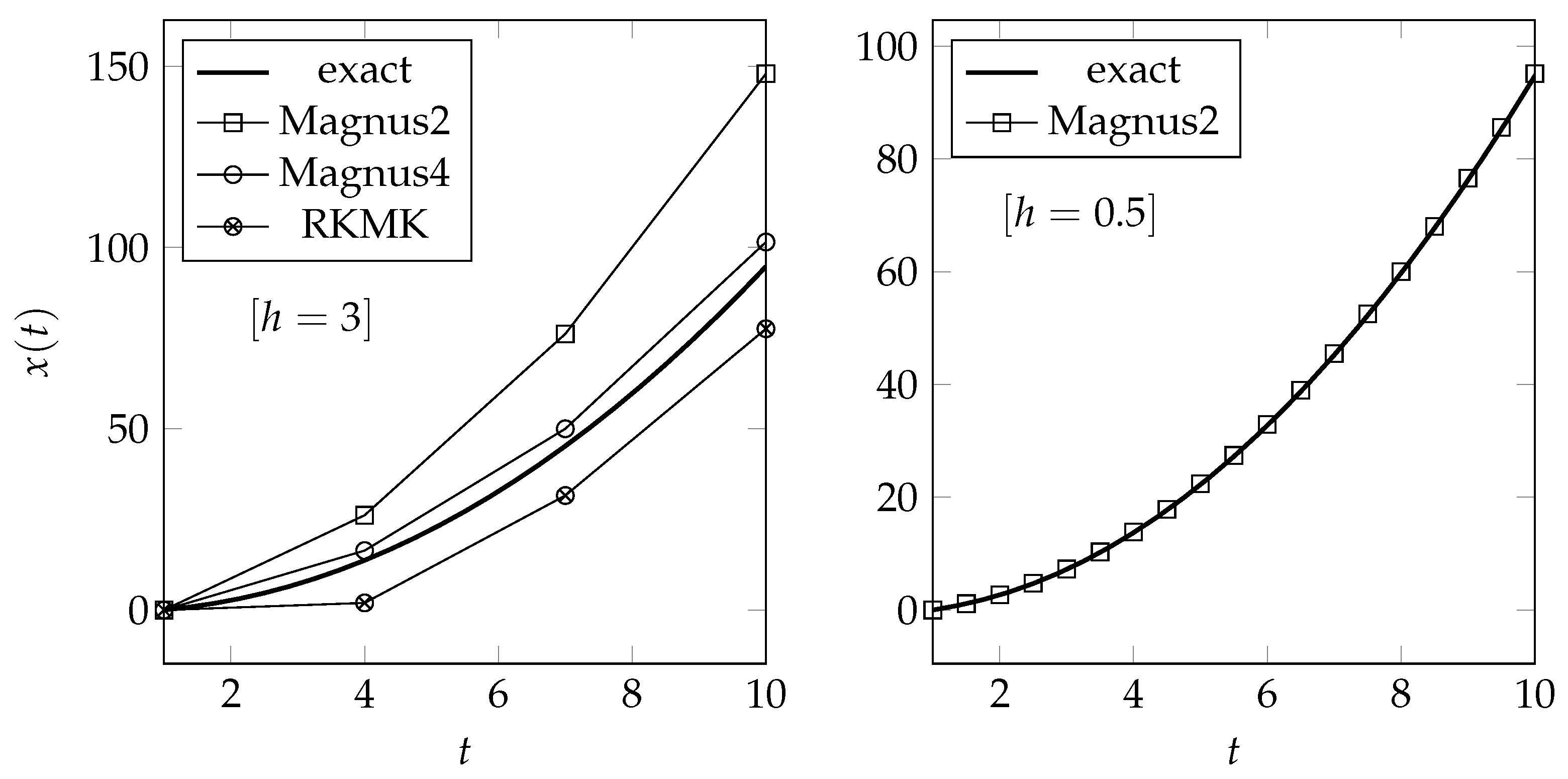
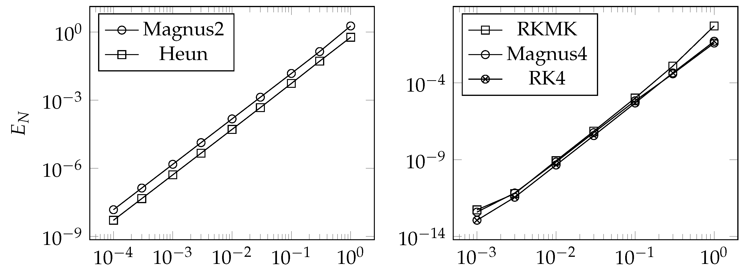
4.1.2. Numerical Example
4.2. SL() and Matrix Riccati Equations
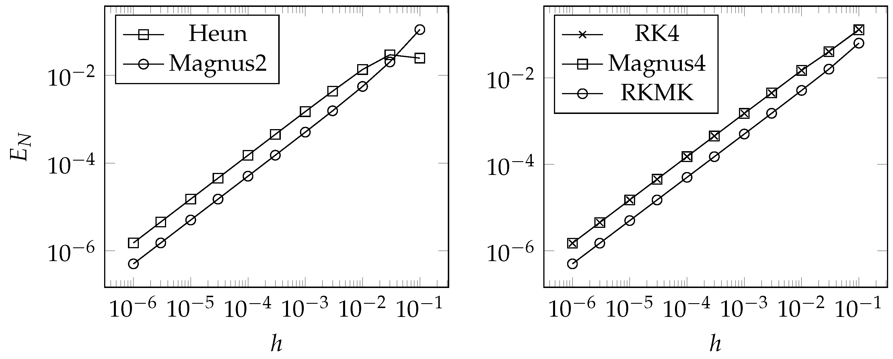
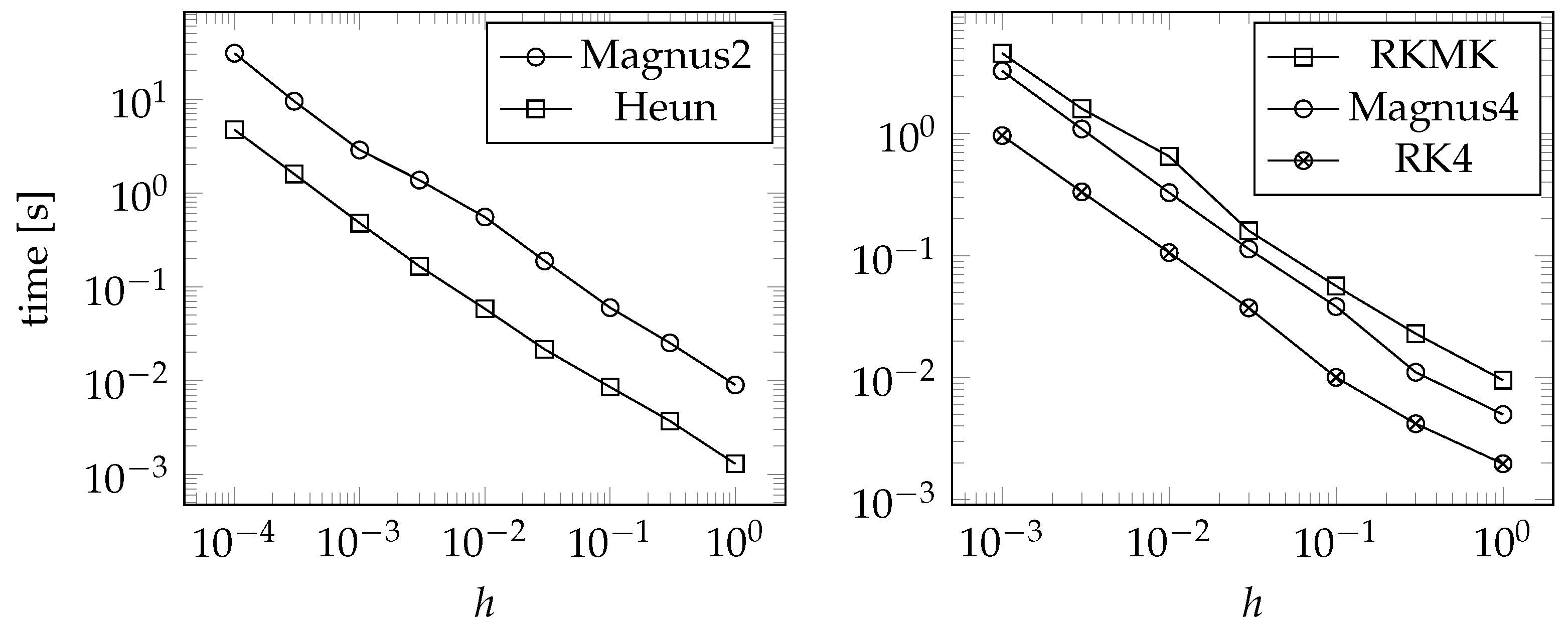
Numerical example
4.3. Generalization to SL()
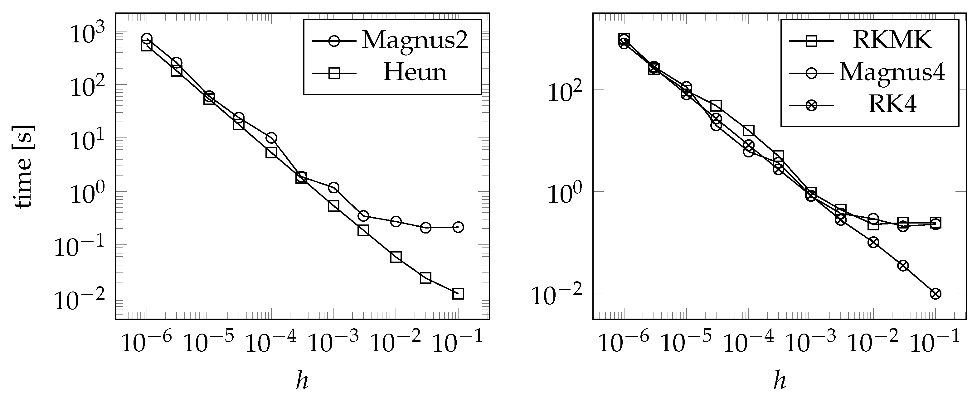
Increase in Numerical Cost as n Increases
5. Applications in Linear Quadratic Control
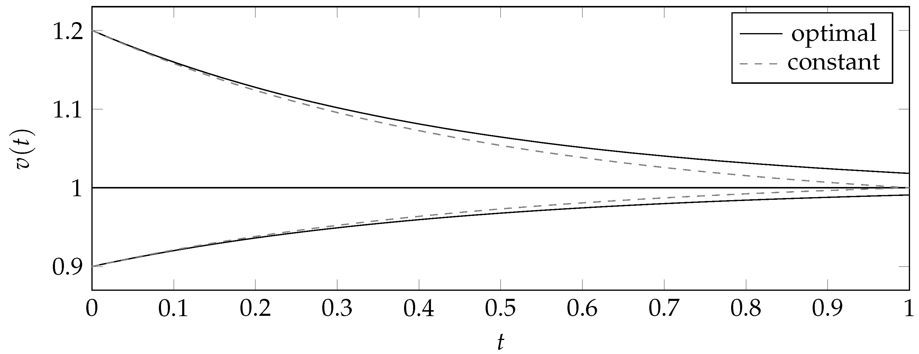
Example: Velocity of a Vehicle
6. Conclusions
Author Contributions
Funding
Institutional Review Board Statement
Informed Consent Statement
Data Availability Statement
Acknowledgments
Conflicts of Interest
References
- Cariñena, J.F.; Grabowski, J.; Marmo, G. Lie-Scheffers Systems: A Geometric Approach; Napoli Series in Physics and Astrophysics; Bibliopolis: Bruxelles, Belgium, 2000. [Google Scholar]
- de Lucas, J.; Sardón, C. A Guide to Lie Systems with Compatible Geometric Structures; World Scientific: Singapore, 2020. [Google Scholar]
- Winternitz, P. Nonlinear action of Lie groups and superposition rules for nonlinear differential equations. Phys. A 1982, 114, 105–113. [Google Scholar] [CrossRef]
- Cariñena, J.F.; Grabowski, J.; Ramos, A. Reduction of t-dependent systems admitting a superposition principle. Acta Appl. Math. 2001, 66, 67–87. [Google Scholar] [CrossRef]
- Cariñena, J.F.; de Lucas, J. Lie Systems: Theory, Generalisations, and Applications. Diss. Math. 2011, 479. [Google Scholar] [CrossRef]
- Sardón, C. Lie Systems, Lie Symmetries and Reciprocal Transformations. Ph.D. Thesis, Universidad de Salamanca, Salamanca, Spain, 2015. [Google Scholar]
- Cortés, J.; Martínez, S. Non-holonomic integrators. Nonlinearity 2001, 14, 1365–1392. [Google Scholar] [CrossRef]
- Iserles, A.; Munthe-Kaas, H.; Nørsett, S.; Zanna, A. Lie-group methods. Acta Numer. 2005, 9, 215–365. [Google Scholar] [CrossRef]
- Marrero, J.C.; Martín de Diego, D.; Martínez, E. Discrete Lagrangian and Hamiltonian mechanics on Lie groupoids. Nonlinearity 2006, 19, 1313–1348. [Google Scholar] [CrossRef]
- Marsden, J.E.; West, M. Discrete mechanics and variational integrators. Acta Numer. 2001, 10, 357–514. [Google Scholar] [CrossRef]
- McLachlan, R.; Quispel, G.R.W. Splitting methods. Acta Numer. 2002, 11, 341–434. [Google Scholar] [CrossRef]
- Sanz-Serna, J.M. Symplectic integrators for Hamiltonian problems: An overview. Acta Numer. 1992, 243–286. [Google Scholar] [CrossRef]
- Pietrzkowski, G. Explicit solutions of the a1-type Lie-Scheffers system and a general Riccati equation. J. Dyn. Control Syst. 2012, 18, 551–571. [Google Scholar] [CrossRef][Green Version]
- Rand, D.W.; Winternitz, P. Nonlinear superposition principles: A new numerical method for solving matrix Riccati equations. Comput. Phys. Commun. 1984, 33, 305–328. [Google Scholar] [CrossRef]
- Cariñena, J.F.; Grabowski, J.; Marmo, G. Superposition rules, Lie theorem and partial differential equations. Rep. Math. Phys. 2007, 60, 237–258. [Google Scholar] [CrossRef]
- Cariñena, J.F.; Ramos, A. Integrability of the Riccati equation from a group theoretical viewpoint. Int. J. Mod. Phys. A 1999, 14, 1935–1951. [Google Scholar] [CrossRef]
- Angelo, R.M.; Wresziński, W.F. Two-level quantum dynamics, integrability and unitary NOT gates. Phys. Rev. A 2005, 72, 034105. [Google Scholar] [CrossRef]
- Lázaro-Camí, J.A.; Ortega, J.P. Superposition rules and stochastic Lie-Scheffers systems. Ann. Inst. H. Poincaré Probab. Stat. 2009, 45, 910–931. [Google Scholar] [CrossRef]
- Hussin, V.; Beckers, J.; Gagnon, L.; Winternitz, P. Superposition formulas for nonlinear superequations. J. Math. Phys. 1990, 31, 2528–2534. [Google Scholar]
- Cariñena, J.F.; de Lucas, J.; Sardón, C. A new Lie systems approach to second-order Riccati equations. Int. J. Geom. Meth. Mod. Phys. 2011, 9, 1260007. [Google Scholar] [CrossRef]
- Cariñena, J.F.; de Lucas, J. Applications of Lie systems in dissipative Milne-Pinney equations. Int. J. Geom. Meth. Mod. Phys. 2009, 6, 683–699. [Google Scholar] [CrossRef]
- Odzijewicz, A.; Grundland, A.M. The Superposition Principle for the Lie Type first-order PDEs. Rep. Math. Phys. 2000, 45, 293–306. [Google Scholar] [CrossRef][Green Version]
- Iserles, A.; Nørsett, S.P. On the solution of linear differential equations in Lie groups. Philos. Trans. R. Soc. A 1999, 357, 983–1020. [Google Scholar] [CrossRef]
- Zanna, A. Collocation and relaxed collocation for the Fer and Magnus expansions. J. Numer. Anal. 1999, 36, 1145–1182. [Google Scholar] [CrossRef]
- Munthe-Kaas, H. Runge-Kutta methods on Lie groups. BIT Numer. Math. 1998, 38, 92–111. [Google Scholar] [CrossRef]
- Munthe-Kaas, H. High order Runge-Kutta methods on manifolds. J. Appl. Numer. Math. 1999, 29, 115–127. [Google Scholar] [CrossRef]
- de Lucas, J.; Grundland, A.M. A Lie systems approach to the Riccati hierarchy and partial differential equations. J. Differ. Equ. 2017, 263, 299–337. [Google Scholar]
- Kučera, V. A Review of the Matrix Riccati Equation. Kybernetika 1973, 9, 42–61. [Google Scholar]
- Lee, J.M. Introduction to Smooth Manifolds; Graduate Texts in Mathematics 218; Springer: New York, NY, USA, 2003. [Google Scholar]
- Ado, I.D. The representation of Lie algebras by matrices. Uspekhi Mat. Nauk. 1947, 2, 159–173. [Google Scholar]
- Curtis, M.L. Matrix Groups, 2nd ed.; Springer: New York, NY, USA, 1984. [Google Scholar]
- Hall, B. Matrix Lie Groups. In Lie Groups, Lie Algebras, and Representations: An Elementary Introduction; Springer International Publishing: Berlin/Heidelberg, Germany, 2015; pp. 3–30. [Google Scholar]
- Sattinger, D.H.; Weaver, O.L. Lie Groups and Algebras with Applications to Physics; Geometry and Mechanics; Springer: Berlin/Heidelberg, Germany, 1986. [Google Scholar]
- Lie, S.; Scheffers, G. Vorlesungen über continuierliche Gruppen mit geometrischen und anderen Anwendungen; Teubner: Leipzig, Germany, 1893. [Google Scholar]
- Levi, E.E. Sulla Struttura dei Gruppi Finiti e Continui. Atti Della R. Accad. Delle Sci. Torino 1905, 40, 551–565. [Google Scholar]
- Hairer, E.; Nørsett, S.P.; Wanner, G. Solving Ordinary Differential Equations I: Nonstiff Problems; Springer: Berlin/Heidelberg, Germany, 1993. [Google Scholar]
- Isaacson, E.; Keller, H.B. Analysis of Numerical Methods; John Wiley & Sons: New York, NY, USA; London, UK; Sydney, Australia, 1966. [Google Scholar]
- Quarteroni, A.; Sacco, R.; Saleri, F. Numerical Mathematics; Springer: New York, NY, USA, 2007. [Google Scholar]
- Magnus, W. On the exponential solution of differential equations for a linear operator. Commun. Pure Appl. Math. 1954, 7, 649–673. [Google Scholar] [CrossRef]
- Iserles, A.; Nørsett, S.P.; Rasmussen, A.F. t-Symmetry and High-Order Magnus Methods; Technical Report 1998/NA06, DAMTP; University of Cambridge: Cambridge, UK, 1998. [Google Scholar]
- Blanes, S.; Casas, F.; Ros, J. Improved high order integrators based on the Magnus expansion. BIT Numer. Math. 2000, 40, 434–450. [Google Scholar] [CrossRef]
- Hairer, E.; Lubich, C.; Wanner, G. Geometric Numerical Integration; Springer: Berlin/Heidelberg, Germany, 2006. [Google Scholar]
- Hartshorne, R. Foundations of Projective Geometry; W.A. Benjamin, Inc.: New York, NY, USA, 1967. [Google Scholar]
- Harnad, J.; Winternitz, P.; Anderson, R.L. Superposition principles for matrix Riccati equations. J. Math. Phys. 1983, 24, 1062. [Google Scholar] [CrossRef]
- Reid, W.T. Riccati Differential Equations; Academic: New York, NY, USA, 1972. [Google Scholar]
- Domínguez, S.; Campoy, P.; Sebastián, J.M.; Jiménez, A. Control en el Espacio de Estado; Pearson: London, UK, 2006. [Google Scholar]
- Sontag, E.D. Mathematical Control Theory: Deterministic Finite Dimensional Systems; Springer: New York, NY, USA, 1998. [Google Scholar]
- Pandey, A.; Ghose-Choudhury, A.; Guha, P. Chiellini integrability and quadratically damped oscillators. Int. J. Non-Linear Mech. 2017, 92, 153–159. [Google Scholar] [CrossRef][Green Version]
- Penskoi, A.V.; Winternitz, P. Discrete matrix Riccati equations with super-position formulas. J. Math. Anal. Appl. 2004, 294, 533–547. [Google Scholar] [CrossRef]
- Herranz, F.J.; de Lucas, J.; Tobolski, M. Lie-Hamilton systems on curved spaces: A geometrical approach. J. Phys. A 2017, 50, 495201. [Google Scholar] [CrossRef]
- Lange, J.; de Lucas, J. Geometric models for Lie–Hamilton systems on . Mathematics 2019, 7, 1053. [Google Scholar] [CrossRef]


| Optimal Control | 10.340 | 5.816 | 2.585 | 0.646 | 0 |
| Constant Control | 11.771 | 6.621 | 2.943 | 0.736 | 0 |
Disclaimer/Publisher’s Note: The statements, opinions and data contained in all publications are solely those of the individual author(s) and contributor(s) and not of MDPI and/or the editor(s). MDPI and/or the editor(s) disclaim responsibility for any injury to people or property resulting from any ideas, methods, instructions or products referred to in the content. |
© 2023 by the authors. Licensee MDPI, Basel, Switzerland. This article is an open access article distributed under the terms and conditions of the Creative Commons Attribution (CC BY) license (https://creativecommons.org/licenses/by/4.0/).
Share and Cite
Blanco Díaz, L.; Sardón, C.; Jiménez Alburquerque, F.; de Lucas, J. Geometric Numerical Methods for Lie Systems and Their Application in Optimal Control. Symmetry 2023, 15, 1285. https://doi.org/10.3390/sym15061285
Blanco Díaz L, Sardón C, Jiménez Alburquerque F, de Lucas J. Geometric Numerical Methods for Lie Systems and Their Application in Optimal Control. Symmetry. 2023; 15(6):1285. https://doi.org/10.3390/sym15061285
Chicago/Turabian StyleBlanco Díaz, Luis, Cristina Sardón, Fernando Jiménez Alburquerque, and Javier de Lucas. 2023. "Geometric Numerical Methods for Lie Systems and Their Application in Optimal Control" Symmetry 15, no. 6: 1285. https://doi.org/10.3390/sym15061285
APA StyleBlanco Díaz, L., Sardón, C., Jiménez Alburquerque, F., & de Lucas, J. (2023). Geometric Numerical Methods for Lie Systems and Their Application in Optimal Control. Symmetry, 15(6), 1285. https://doi.org/10.3390/sym15061285