1. Introduction
Topology optimization refers to the process of finding the optimal distribution of materials within a given design area. Since the “homogenization method” was proposed in one study [
1], it has attracted attention widely from scholars. After more than 30 years of development, topology optimization has developed rapidly. The Bi-directional Evolutionary Structural Optimization (BESO) [
2] method is the most typical solution method for continuous structure topology optimization. The BESO method discretized the design variables into groups titled 0 and 1, so there was no intermediate density unit and the topology result would not be blurred or unclear. This method is widely used in the engineering field because of its simple algorithm and convenient programming [
3]. For example, Xu [
4] established a multi-material periodic structure problem model and used the BESO method to solve the problem. The final results showed that BESO could successfully solve the optimal topology structure of the problem, and the performance of the topology configuration was indeed improved. The BESO method can be extended to present similarities with the design method of elastic phonon crystal by taking the attenuation factor of the wave at a specified frequency as the objective function and the target volume and target stiffness as the constraint conditions [
5]. This is completed in order to improve the crashworthiness of thin-walled square tubes under axial compressive loads. With the minimum volume as the objective function and the energy absorption constraint as the constraint condition, the topology optimization results of thin-walled square tubes can be obtained. This result can improve the performance of thin-walled square tubes in terms of peak crushing force [
6].
Although BESO has achieved success in many engineering fields, the BESO method also has some problems that need to be solved. It needs to reach a preset target volume for each iteration optimization and a fixed number of elements must be deleted, which may cause the deletion of elements mistakenly or wrongly. This may result in issues of not finding the optimal material distribution in the structure and falling into a local optimum easily. The most suitable approach to address the emergence of such a problem is to solve the BESO model problem using a meta-heuristic algorithm [
7].
At present, many scholars have studied the use of meta-heuristic algorithms to solve the problem of the topology optimization model. However, many mathematicians are studying meta-heuristic algorithms designed to solve discrete topology optimization, such as Degertekin [
8], Dang [
9], Li [
10] and Ma [
11]. Only a few scholars have studied the problem of meta-heuristics and continuum topology optimization. Luh [
7], Kaveh [
12] and Yoo [
13] all used an improved ant colony algorithm to solve the issues of the topology optimization model; Ahn [
14] used an improved BB-BC algorithm; Tseng [
15] and Zuo [
16] used a particle swarm algorithm and a genetic algorithm, respectively. There are similar problems in the above literature. There are some problems of high cost and low efficiency in regard to solving topology optimization models using meta-heuristic algorithms. Its principle is that the objective function of topology optimization is directly taken as the fitness function of the meta-heuristic algorithm in this method, which leads to a large number of finite element analyses and calculations in the process of topology optimization. At the same time, these meta-heuristic algorithms were proposed earlier and there are some bottlenecks in their performance.
Generally speaking, the common method of using the meta-heuristic algorithm to solve the model problems is to form a population composed of N individuals, iteratively update these populations and end the iteration until the convergence conditions are met, then output and obtain the optimal value. However, this method is not the best choice for topology optimization of a continuum structure. The most important performance evaluation indicators of an optimization algorithm are computational efficiency and computational accuracy. The most time-consuming part of the topology optimization algorithm is the number of finite element analyses, and it can be said that the calculation time is approximately equal to the number of finite element analyses. The continuum topology optimization is designed to discretize the whole structure into M elements, which means that a finite element analysis of M elements is required for each iteration. Taking the BESO method as an example, only one finite element analysis of M elements is required for each iteration. If the meta-heuristic algorithm is used to solve the topology optimization model, for example, for a population composed of N individuals, in each iteration, N times of finite element analysis on M elements are needed. With the expansion of the grid size, that is, the M value, the corresponding N value will also increase in order to ensure the calculation accuracy. This means that using a meta-heuristics algorithm to solve topology optimization problems will greatly increase the computational cost. In order to avoid this problem, this paper uses sensitivity information to guide the meta-heuristic algorithm to solve the issues of the topology optimization model.
The value range of the design variables of the BESO topology optimization model is {0.0001–1}, which is similar to those of integer programming problems, such as “0–1” programming problems. Therefore, it is very suitable to solve the issues of the BESO topology optimization model by using a discrete binary meta-heuristic algorithm.
In order to solve the above problems, this paper studies how to discretize the standard HPO algorithm into a binary HPO algorithm and how the BHPO algorithm solves the topology optimization model of BESO with the help of the guidance of sensitivity information.
This paper is arranged as follows. The first section focuses on the standard HPO algorithm and uses the Sigmoid function to perform discrete binary processing to obtain the binary HPO algorithm. In the second section, the BHPO algorithm is combined with BESO topology optimization to establish the BHPO-BESO topology optimization theory. With the help of the sensitivity information to guide the search direction and the meta-heuristic update principle of the BHPO algorithm, a semi-randomly search for the optimal topology configuration is carried out. In the third section, three typical examples of the cantilever beam, simply supported beam, and clamped beam are used as optimization objects to carry out the numerical simulation experiments, and the results are compared with the solution results of BESO topology optimization, which proves the feasibility and effectiveness of the BHPO-BESO method.
2. Binary HPO Algorithm
The standard Hunter–prey optimization (HPO) algorithm is a recently proposed meta-heuristic algorithm intended to solve continuous optimization problems. This algorithm is inspired by the predatory behaviors between the predator animals, such as lions, leopards, and wolves, and the prey, such as deer, stags, and gazelles. The specific principle and calculation method can be referred to Naruei [
17].
According to Naruei [
17], the standard HPO algorithm has a good performance in terms of solving continuity problems, but due to the particularity of discrete problems, the continuous HPO algorithm cannot obtain a perfect solution. The “0–1” problem is a typical integer programming problem, and its mathematical model and constraints are shown in Equation (1):
where
D is the total number of items,
xi is the
i-th item selected by the traveler, the corresponding weight is
, the value is
qi, and
V represents the maximum load.
Since the “0–1” problem restricts each dimension of the variable to 0 or 1, it is obviously inappropriate to use a continuous algorithm to solve the model; a binary discrete algorithm is more suitable to use to solve this type of problem. In this paper, a binary HPO algorithm is proposed, which can effectively solve the “0–1” problem that makes the standard HPO algorithm unsuitable for solving discreteness.
The generation method of the initial population is shown in Equation (2):
where
xi is the position of the
i-th dimension in each individual, and
R1 is a random generated in the range of [0–1]. When the population is initialized, the position of each dimension of each individual in the population consists of 0 or 1. Whether this position is 0 or 1 is determined by a random number between 0 and 1 generated by this position. If the random number is greater than 0.5, this position is 1; otherwise, this position is 0.
The meta-heuristics algorithm has many ways to extend the continuity algorithm into a binary algorithm, but the easiest and most effective way is to use a transfer function [
18]. A transfer function can map the continuous real values of the input to values between 0 and 1. There are many kinds of transfer functions; here, we use the Sigmoid function, which is the most commonly used transformation function. The specific equation is shown in Equation (3):
where
x(
t + 1) is the hunter or prey position for the next iteration. Although the individuals in the population have been normalized by the transfer function, we still need to convert these mapped values between [0–1] to binary values using Equation (4):
where
R2 is a randomly generated constant in the range [0–1].
When the position of the hunter or prey is updated by the standard HPO algorithm each time, the binary solution can be efficiently obtained via discrete processing using Equations (14) and (15). The binary Hunter–prey optimization (BHPO) algorithm still maintains the characteristics of the standard HPO algorithm. The flow of the BHPO algorithm is described in Algorithm 1.
| Algorithm 1. BHPO algorithm. |
| Input: various parameters |
| Output: The best fitness value and the corresponding individual |
| %%Algorithm running starts |
| Randomly initialize the population using Equation (2) |
| Calculate the fitness function of all individuals |
| Find the safest location for prey |
| it = 0 |
| While it < MaxIt |
| Main part of the HPO algorithm |
| Use Equation (3) to map continuous real values to the range [0, 1] |
| Use Equation (4) to discretize the mapped values into 0 or 1 |
| Calculate the fitness function of all individuals |
| Find the best fitness value compared to the previous iteration |
| Keep the individual position corresponding to the best fitness value |
| Store the best fitness value for each generation iteration |
| it = it + 1 |
| End |
| %%Algorithm running ends |
In order to test the performance of the BHPO algorithm, the “0-1” problem model in Martello [
19] is selected and compared with the BALO and improved BALO algorithms proposed in Zhao [
20]. The model is shown in Equation (1) and the relevant parameter settings are shown in
Table 1. The BHPO algorithm runs independently for 30th. The average fitness value iteration curve is shown in
Figure 1 and the relevant parameters are shown in
Table 2.
3. Topology Optimization of Continuum Structure Based on BHPO Algorithm
3.1. BESO Method
Topology optimization refers to finding a suitable structural design for the existing design model under the specified working conditions and constraints. The model for minimizing compliance under target volume constraints is given by Equation (5):
where
is the design variable in the topology optimization model,
n is the total number of elements in the design area,
p is the penalty factor,
V* is target volume,
Ve is the volume of the
e-th element,
F is the load vector,
U is the displacement vector, and
C is the average compliance of the structure that is the strain energy of the structure. In order to prevent the overall stiffness matrix
K from becoming a singular matrix in the process of topology optimization,
is generally set to 0.0001. In addition,
ke is the element stiffness vector, and
ue is the column vector of element displacement.
Since the principle of topology optimization is to discretize the overall structure into multiple tiny element structures, an interpolation model is usually used to reconstitute the tiny element structures into the overall structure. This paper selects the SIMP interpolation model presented in Andreassen [
21] and the specific equation is shown in Equation (6):
where
E is the elastic modulus of the overall structure,
Emin is the elastic modulus of the blank element and takes a small positive value to ensure the non-singularity of the overall stiffness matrix, and
E0 is the initial elastic modulus of the solid element.
The sensitivity value of an element represents its contribution to the overall structural stiffness, which is related to the deletion and retention of elements and determines the topological shape of structural optimization. The calculation method is shown in Equation (7):
In order to avoid the influence of grid dependence and the checkerboard format on the optimization of the SIMP interpolation model, sensitivity filtering technology is usually adopted. Here we choose the sensitivity filtering technique outlined in Huang [
22].
Node sensitivity is a weighted average of the sensitivity of the elements around the node, as shown in Equation (8):
where
m is the total number of nodes in the filtering range,
rij is the distance between the center of element
i and node
j, and
is the weight of the element. The weight
increases with the decrease of
rij, and the element closer to the node occupies more weight
the greater the influence of this element on the sensitivity of the node.
The method of converting the node sensitivity value into the element sensitivity value is shown in Equation (10):
where
A is the total number of elements connected to node
j and
is the weight of the element sensitivity. The larger the value of
, the closer the node is to the element, and the greater the influence of the sensitivity value of the node on the sensitivity value of the element.
In order to prevent sudden changes in the structure and other phenomena, it is necessary to combine the sensitivity of adjacent two-step elements to correct the current sensitivity value. The correction principle is shown in Equation (12):
where
is the element sensitivity value of this iteration and
is the element sensitivity value of the last iteration.
Topology optimization is a process of iteratively updating design variables until volume constraints and convergence criteria are satisfied. The relevant convergence criterion is shown in Equation (13):
where
τ is the convergence accuracy,
k is the number of iteration steps, and
N is a constant that is generally taken as 5. The iteration can be terminated when the average compliance of the structure changes less than the convergence accuracy in more than 10 consecutive iterations.
3.2. Topology Optimization Based on BHPO Algorithm
Usually, the information condition of sensitivity is used to solve topology optimization problems. The sensitivity information can fully reflect the performance of the objective function, which can reduce the computational cost, improve the computational efficiency, and can also suppress numerical instability through the sensitivity filtering technique. Therefore, it is more appropriate to use the sensitivity information to guide the BHPO algorithm to solve the topology optimization problem.
3.2.1. The Principle of the BHPO-BESO Method
Generally, Equation (5) is used as a fitness function to solve the issues of the topology optimization process via a meta-heuristic algorithm. In this method, the individuals in BHPO represent the entire design space of the structure. During the algorithm iteration process, multiple design spaces need to be iteratively solved and calculated. This will greatly increase the computational cost of topology optimization and increase the amount of finite element calculation involved in topology optimization. Therefore, the sensitivity function is used as the fitness function of the BHPO algorithm in this paper. In other words, Equation (7) is taken as a representative of the fitness function of HPO.
The BHPO-BESO algorithm treats all design variables of topology optimization as an overall population, and each individual is a dimension of the design variables. A double encoding operation is used for each element’s structure, with 0 used for empty elements and 1 used for solid elements. Each element can be composed of a string of binary codes. This binary code has no actual physical meaning but is simply the basis for the BHPO algorithm to update the population information. The empty elements are defined as a binary code consisting of all 0 s, with the solid elements defined as a binary code consisting of the same number of 0s and 1 s. This is shown in
Figure 2. The sensitivity function is the fitness function of HPO, and each character in the binary encoding is the individual of BHPO. Each element is removed and added by updating the binary code. The BHPO algorithm calculates that the best-performing individual (solid element) has more 1 characters, and the worst-performing individual (empty element) has more 0 characters.
3.2.2. Control of Volume Constraints
Regarding the problem of volume constraints in Equation (16), according to Zuo [
16], the concept of “mutation” is cited in the BHPO-BESO algorithm. After the algorithm solves the sensitivity value and passes through the sensitivity filtering technique, all individuals in the population are arranged in descending order of sensitivity value and the entire population is divided into two classes, “superior” and “inferior”. During the mutation operation, when the individuals of the superior population update the binary code, only the transition from 0 to 1 occurs; when the individuals of the inferior population update the binary code, only the transition from 1 to 0 occurs. The size of the superior population is set to
and the remaining populations are all defined as inferior populations. Among them,
N is the number of populations and
volfrace is the volume optimization score set in topology optimization. The mutation factor is shown in Equation (14):
where
Pm is the mutation factor;
Pm0 is the minimum value of the mutation factor;
Pm_max is the maximum value of the mutation factor, which is set to 1; and pen is the penalty coefficient, which is set to 2 in this paper. In addition,
Prog is the optimization volume progress indicator and its calculation method is shown in Equation (15):
where
V0 is the initial volume,
V is the current volume, and
V* is the optimized target volume.
3.2.3. Individual Selection Method of BHPO-BESO
The process of individual selection is based on the number of 1 characters in the binary code. If the binary code of an empty element contains a certain proportion of 1 characters, the empty element is converted to a solid element. If the binary code of a solid element contains all 0 s, the element is converted to an empty element. In this article, the proportion threshold is set to 50%.
The individual selection for the BHPO-BESO algorithm is shown in Equation (16):
where
is the value of the
k-th iteration of the e-th design variable,
is the value of the (k − 1)-th iteration of the e-th design variable, and
H represents the ratio of “1” to the length of the binary code.
3.2.4. The Steps of the BESO-BHPO Algorithm
The overall optimization process of BHPO-BESO is shown below.
Step 1: Determine design-model-related parameters for topology optimization. The overall structure is encoded, the solid elements adopt “1” for binary encoding, and the empty elements adopt “0” and “1” for binary mixed encoding;
Step 2: Set topology-optimization-related parameters;
Step 3: Perform finite element analysis on the structure and extract sensitivity information values;
Step 4: Correct the sensitivity information and perform filtering calculations;
Step 5: Sort the sensitivity values in descending order to divide the population class;
Step 6: Use the BHPO algorithm to update the population;
Step 7: Update the population using mutation operations;
Step 8: Determine whether the current iteration conditions of the BHPO algorithm are met. If this step is not satisfied, go to Step 6; if it is satisfied, go to Step 9;
Step 9: Update design variables;
Step 10: Determine whether the optimization target volume and convergence conditions are satisfied. If satisfied, stop the iteration, if not, return to Step 3.
The flow chart of BHPO-BESO is shown in
Figure 3.
4. Numerical Examples
In this section, three classical model examples of the simply supported beam, cantilever beam, and clamping beam are used to verify the feasibility and effectiveness of the BHPO-BESO algorithm and compare it with the traditional BESO algorithm. In the previous literature, few people have verified the validation process of the algorithm for large-size grid examples. Therefore, this paper comprehensively considers the balance between computational efficiency and large-size grids and selects three calculation examples with the number of grids of three different sizes, respectively, to verify whether different grid sizes would affect the BHPO-BESO optimization results. Considering the randomness of the BHPO-BESO algorithm, each model example is run 20 times independently. The maximum number of iterations of BHPO is set to 10. Considering the balance between computational efficiency and computational precision, the binary encoding length is set to 10.
4.1. Example of Simply Supported Beam Model
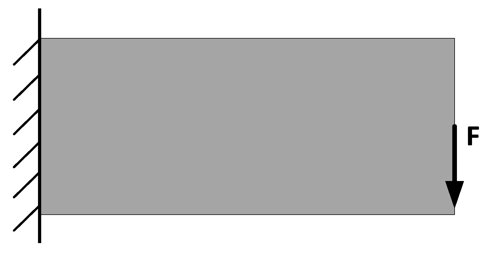
Figure 4a shows the initial design area of the simply supported beam model.
The initial design model of the structure in Example 1 is the rectangular simply supported beam model of
. The upper middle position is subjected to a vertical downward concentrated load F with a value of 20 N, the lower left corner of the model is constrained by the degrees of freedom in the X and Y directions, and the lower right corner is constrained by the Y direction. Considering that the simply supported beam model is an axisymmetric graph, its structure is also symmetrical. Therefore, in order to improve the computational efficiency, only the right half of the structure in
Figure 4b is designed for topology optimization. The structure of the right half is discretized into a
element, whose mesh size is
.
The parameter settings are as follows. The minimum mutation factor
Pm0 = 0.6, the penalty factor
p = 3, the filter radius
rmin = 3, the evolution rate
ER = 0.02, the Young’s elastic modulus
E = 206 GPa, the Poisson’s ratio of the material is set to 0.3, and the convergence accuracy
= 0.001. The parameters of the two topology optimization algorithms are set the same and the topology optimization results are shown in
Figure 5 and
Table 3.
According to
Figure 5, the main structure of the topological configuration solved by the BHPO-BESO algorithm with 20 independent operations is similar to the structure solved by BESO. The difference between the two is that the topological configuration solved by BHPO-BESO reduces more fine mesh branch structures than BESO. At the same time, due to the idea of the BESO method, the BHPO-BESO optimization results only have the two values of 0.0001 and 1, which avoids the existence of intermediate density elements and makes the optimization results more manufacturable. The following conclusions can be drawn from the data in
Table 3. A total of 19 optimal topological configurations were searched via BHPO-BESO in 20 operations and the probability of obtaining the optimal topological configuration was 90%. The average number of iteration steps was reduced by 6.2 times compared with that of BESO, accounting for 14.09% of the original iteration step size. The mean compliance value was 0.0937 lower than that of BESO. This indicates that the BHPO-BESO algorithm needs fewer instances of finite element analysis than the BESO algorithm and has a faster convergence speed and higher computational efficiency. Meanwhile, it can also find topology configurations with smaller average compliance (i.e., greater stiffness) than the BESO algorithm. In order to more intuitively reflect the differences between the two,
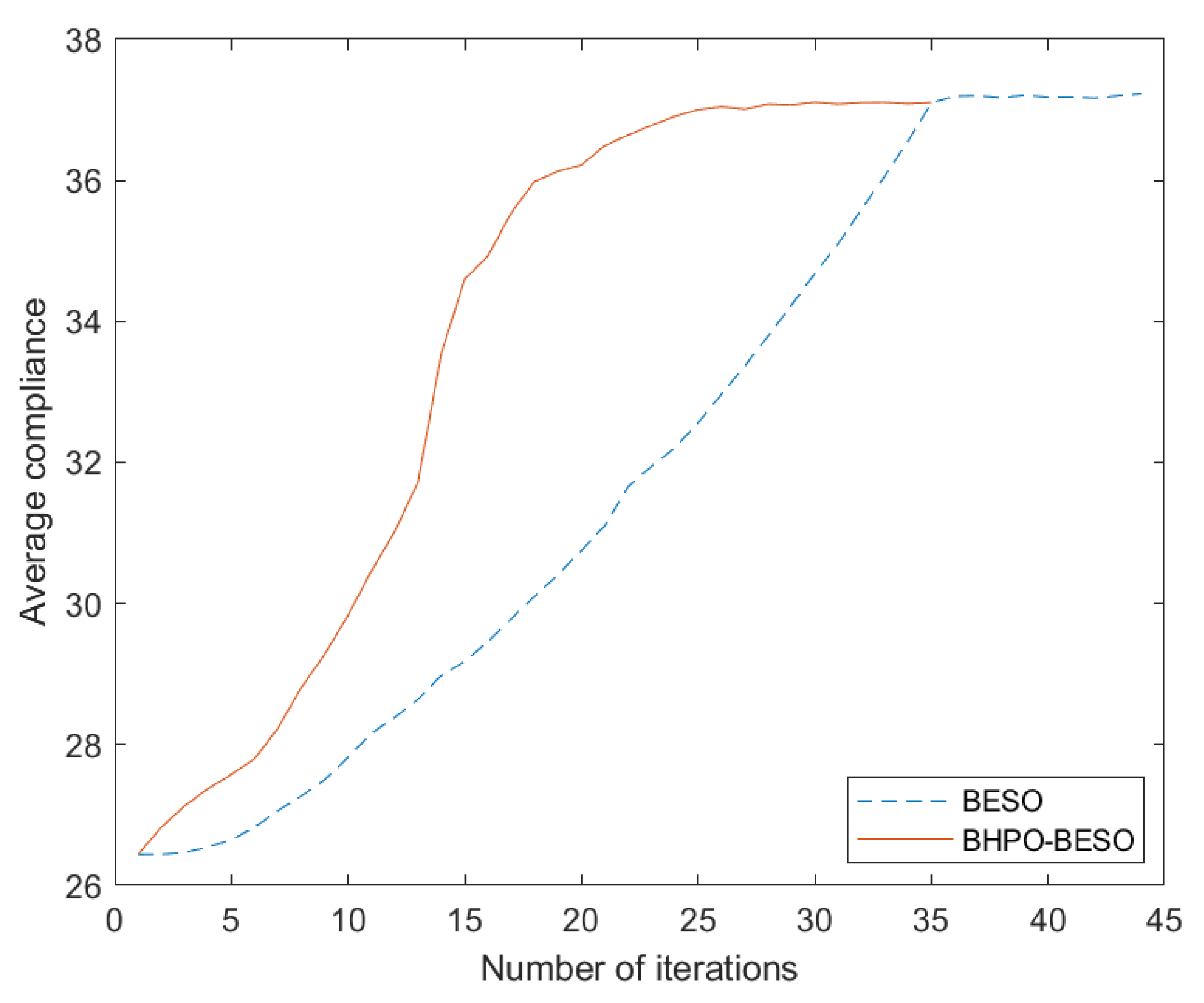
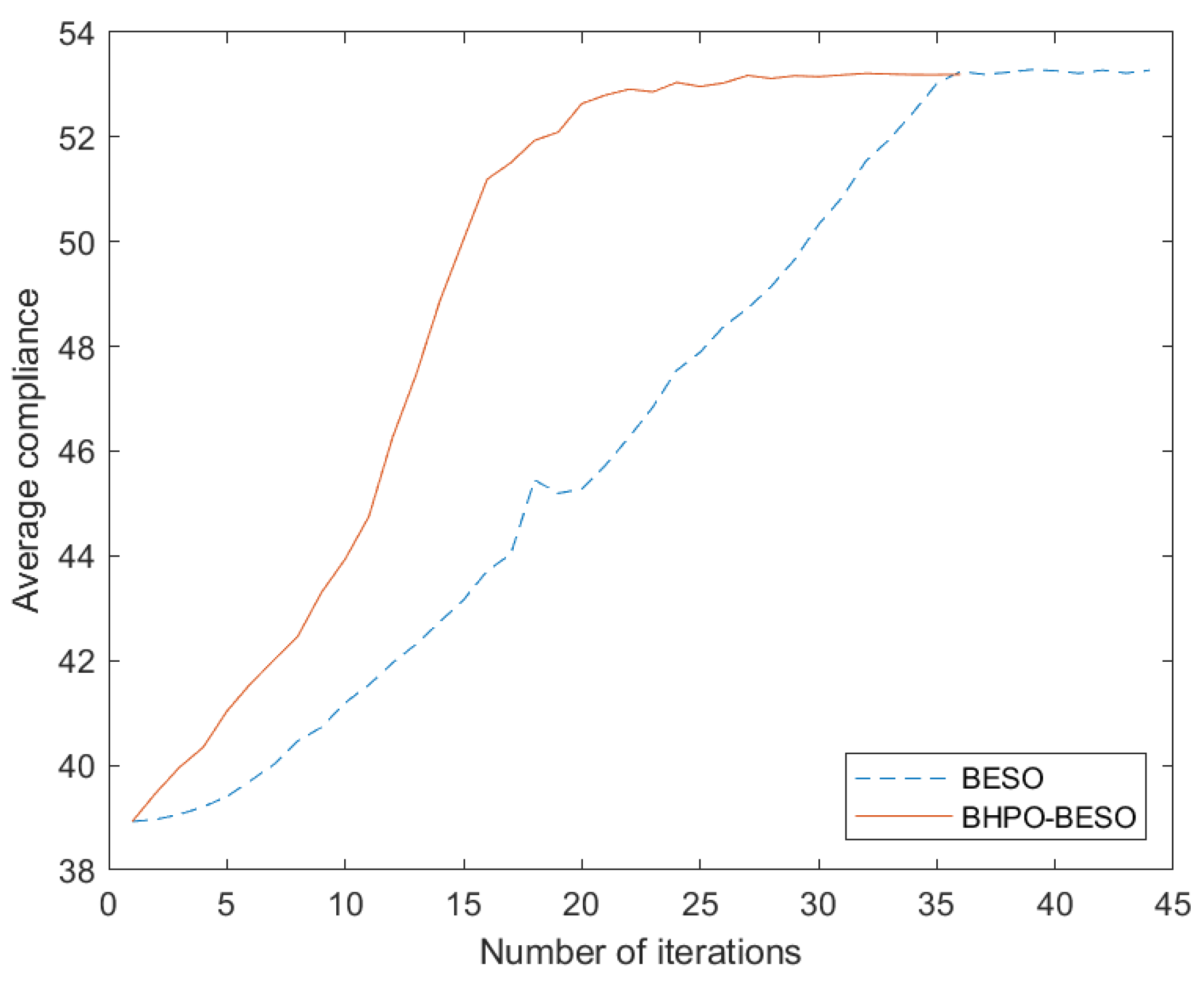
Figure 6 shows a comparison of the iterative processes of BHPO-BESO and BESO.
Due to the gradual removal of inefficient materials to meet the set volume constraints, the structural compliance value first continues to increase, and after reaching the volume constraint, continues to search for the minimum compliance value under this target.
Through the calculation of the simply supported beam model, the topological configurations obtained by BHPO-BESO under three different mesh sizes are improved to different degrees compared with the BESO method, indicating that the BHPO-BESO algorithm has good adaptability to the mesh size. The results of each optimization may be different due to the randomness of BHPO-BESO. However, there is at least a 90% probability that a better topology can be obtained via this method than the BESO method and that its computational efficiency can be higher than that of the BESO method.
4.2. Example of Cantilever Beam Model
The cantilever beam model is set up with 3 different mesh numbers
,
, and
.
Figure 7 shows the initial design area of the cantilever beam.
The initial design model of Example 4 is the cantilever beam of The middle position of the rightmost end bears a vertical downward concentrated load F with a value of 20 N and the leftmost end is constrained by the degrees of freedom in the X and Y directions.
The parameter settings are as follows. The mutation factor P
m0 = 0.6, the penalty factor
p = 3, the filter radius r
min = 3, the evolution rate ER = 0.02, the Young’s modulus of elasticity E = 206 GPa, the Poisson’s ratio of the material is set to 0.3, and the convergence accuracy τ = 0.001. The parameters of the two topology optimization algorithms are set the same and the topology optimization results are shown in
Figure 8 and
Table 4.
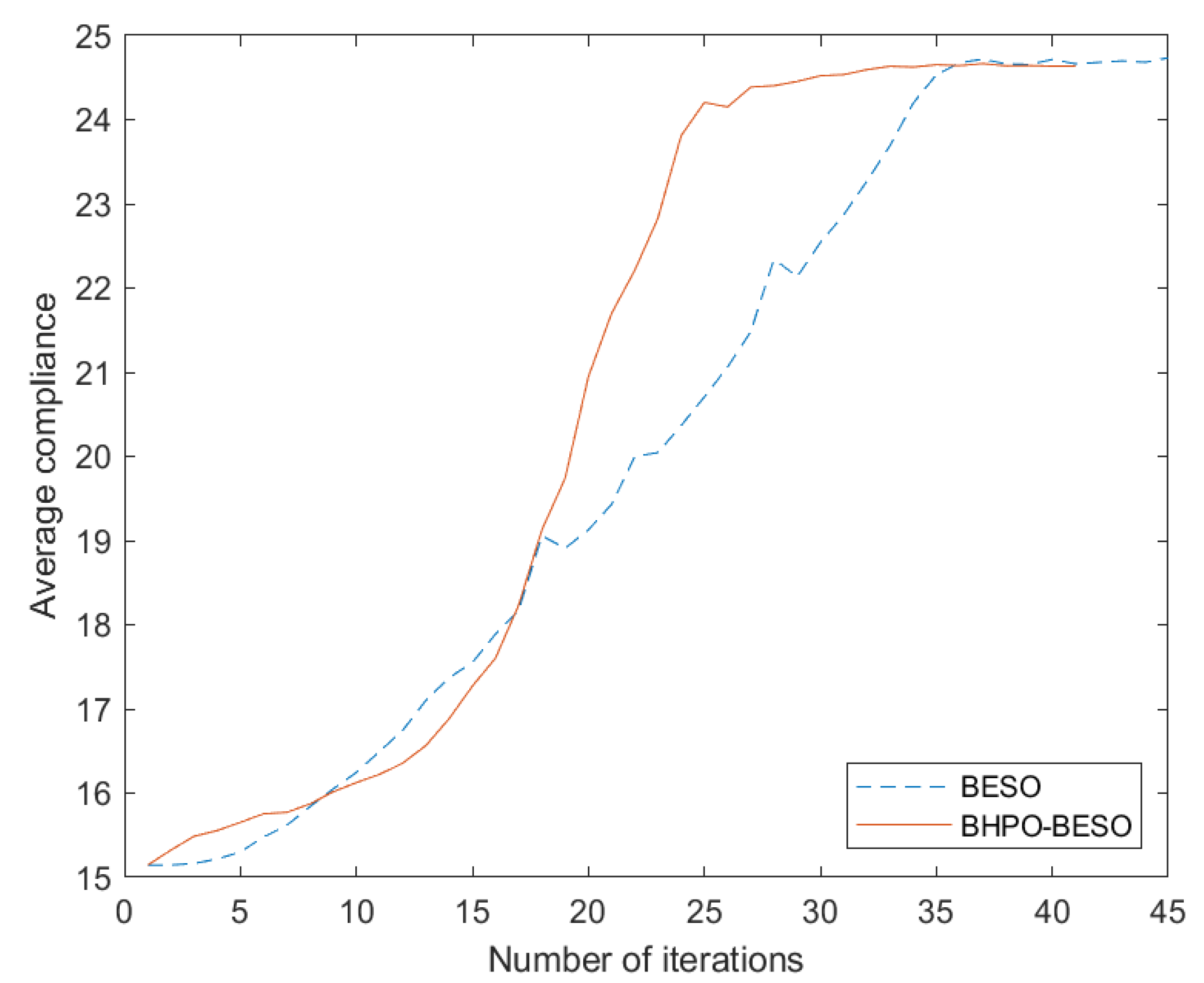
It can be seen in
Figure 9 that both of them have oscillations in the iterative process. Due to the fact that deleting materials during the optimization process can cause certain connections of the structure to break and change, resulting in structural mutations, the compliance value curve sometimes experiences a jump increase phenomenon. After the structure generates new connections and forces transmission paths, the compliance value quickly returns to its normal state and the optimization process still follows the correct direction.
Through the cantilever beam example, we obtained that BHPO-BESO can still obtain the optimal topology configuration compared with the BESO method being unable to and it has better computational efficiency. The optimization results under the three different grid sizes show that the BHPO-BESO algorithm has good adaptability to the grid size.
4.3. Clamping Beam Model Example
The clamping beam model is set with 3 different mesh numbers
,
, and
.
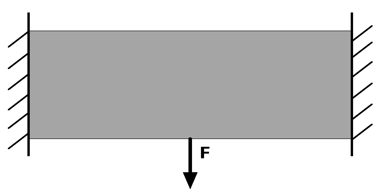
Figure 10 shows the initial real area of the clamping beam. The middle position of the lowermost end bears a vertical downward concentrated load F with a value of 60N, and the leftmost side is constrained by the degrees of freedom in the two directions of X and Y.
The number of grid sizes in Example 7 is set to
The minimum mutation factor
Pm0 = 0.6, the penalty factor
p = 3, the filter radius
rmin = 2, the evolution rate
ER = 0.02, the Young’s modulus of elasticity
E = 206 GPa, the Poisson’s ratio of the material is set to 0.3, and the convergence accuracy
τ = 0.001. The parameters of the two topology optimization algorithms are set the same, and the topology optimization results are shown in
Figure 11,
Figure 12 and
Table 5.
In the clamping beam model, unlike the previous two example models, the optimal topological configuration solved by BHPO-BESO is similar to the configuration solved by BESO, even at different sizes. The optimal number of topological configurations obtained by running BHPO-BESO 20 consecutive times under grid scales of different sizes are 19, 20, and 20, respectively. Compared with BESO, the average number of iteration steps of BHPO-BESO decreased by 9.75, 10.7, and 6.95, accounting for 22.16%, 24.32%, and 16.16% of the number of iteration steps of BESO; the average compliance decreased by 0.0755, 0.0272, and 0.0318. Since both of the first two examples use an initial mutation factor of 0.6, which is higher than the latter’s initial mutation factor of 0.5, the convergence speed of the first two examples is also faster than that of the latter. The following conclusions are drawn from the above data. In the clamping beam example, the calculation efficiency and the compliance are improved.
The topology results of the example show that the final topology result will appear as asymmetry in the problem design with symmetry. This is due to the randomness of the BHPO algorithm. In terms of the application of meta-heuristic algorithms to engineering optimization problems, the final results are often not unique. It is because of the randomness of the meta-heuristic algorithm that the engineering optimization problem is given a wider search space. However, methods for how to avoid this phenomenon in future work is worth thinking about and further studying.
5. Finite Element Simulation Analysis
As displayed above, we have used MATLAB software to test relevant examples. In order to further verify the effectiveness of BHPO-BESO, this section carries out a static finite element simulation for the topological configuration obtained in the previous section. The finite element simulation platform uses Comsol software. Here, one of the three examples in the above section is selected for the experiment.
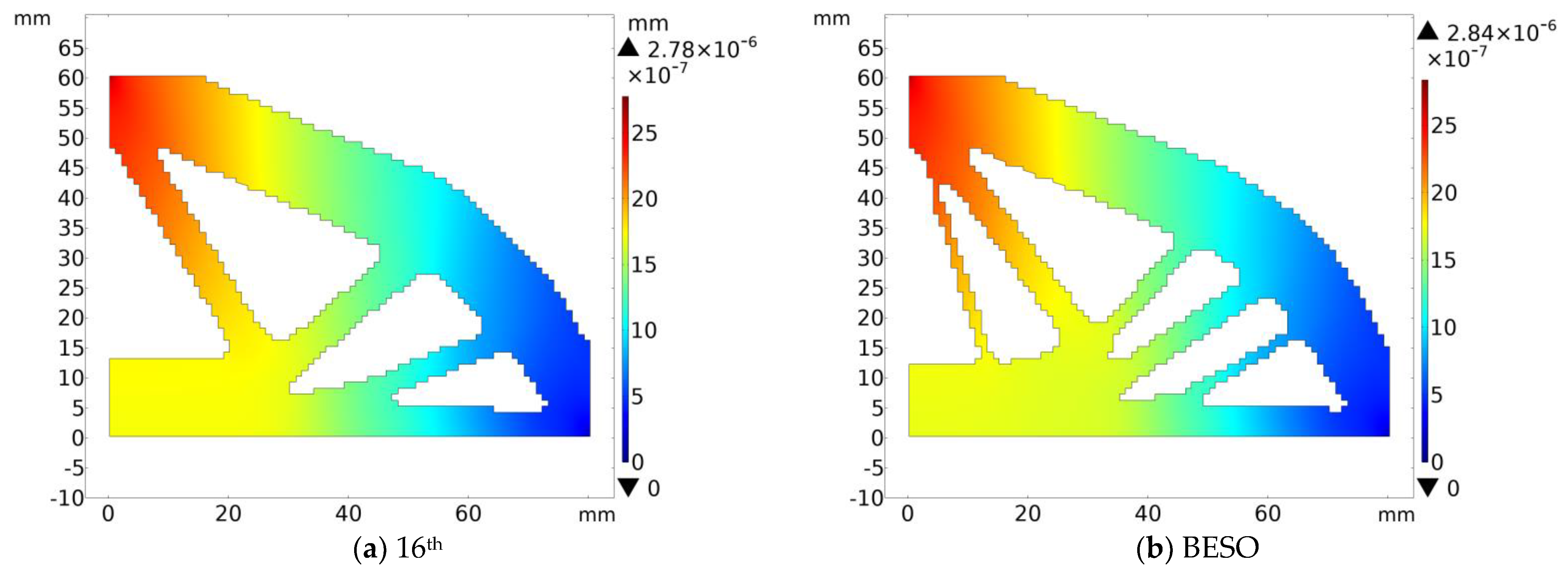
Firstly, the 16th topological configuration in the simply supported beam (80*60) example and the corresponding BESO topological configuration were selected for simulation analysis and comparison. The boundary conditions and parameters of all simulations are the same as those set in MATLAB. The result is shown in
Figure 13.
The finite element simulation analysis results reveal several differences. Under the same boundary conditions and parameters, the maximum deformation displacement of BHPO-BESO and BESO are 2.78 × 10⁻⁶ mm and 2.84 × 10⁻⁶ mm, respectively. The maximum deformation displacement of BHPO-BESO is 2.1% less than that of BESO.
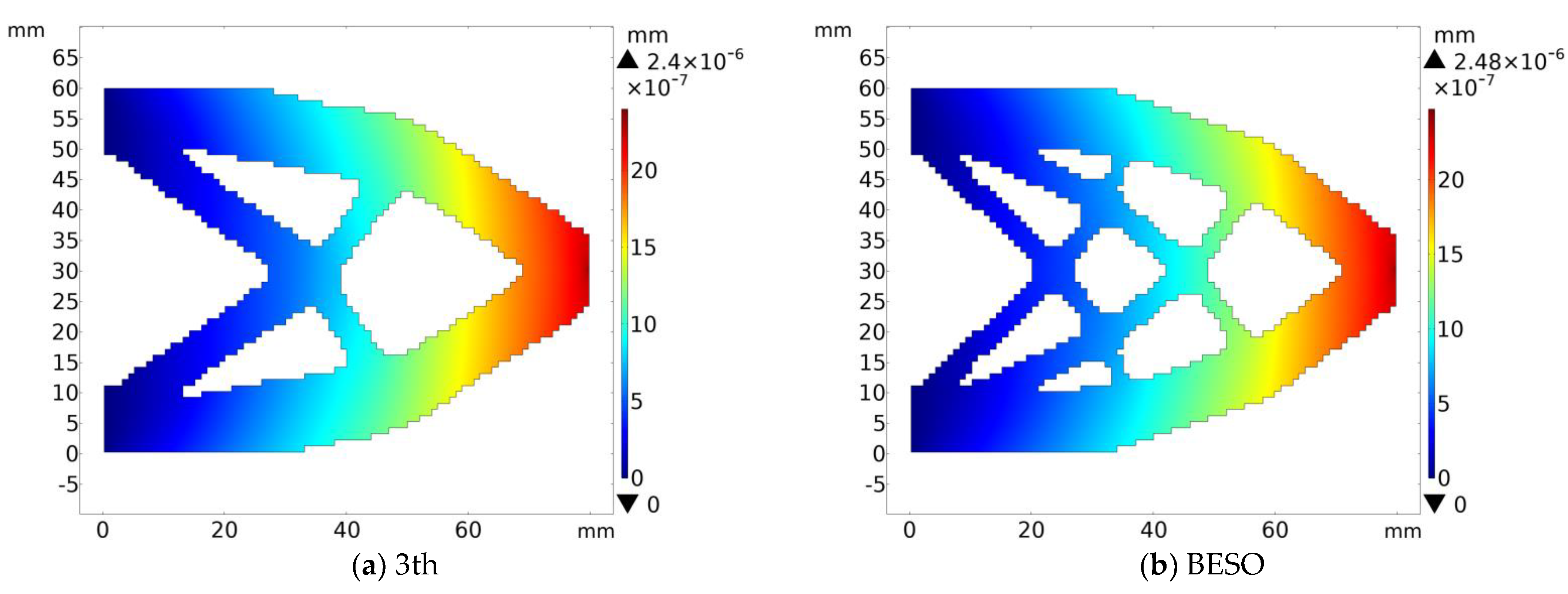
In the cantilever beam calculation example, the 3rd topology configuration and the corresponding BESO topology configuration are selected for finite element simulation and comparative analysis. The result is shown in
Figure 14.
In the cantilever beam finite element simulation experiment, the maximum deformations of the BHPO-BESO and BESO topologies are 2.4 × 10⁻⁶ mm and 2.48 × 10⁻⁶ mm, respectively, and their maximum deformation displacement is reduced by 3.2%.
In the example of the clamping beam, the 14th topological configuration is selected and the finite element simulation experiment is carried out with the corresponding BESO topological configuration. The result is shown in
Figure 15.
In terms of the clamping beam, it can be found that the maximum deformation displacement of BHPO-BESO, relative to BESO topology, decreases by 1.2%.
The final results of the three sets of finite element simulation experiments in this section show that the topological configuration solved by BHPO-BESO has greater stiffness than that of the BESO algorithm, which further illustrates the effectiveness of the BHPO-BESO algorithm.
6. Conclusions
This paper mainly proposes that the binary HPO algorithm and a new topology optimization theory with BHPO-BESO could efficiently find the optimal topology configuration. In view of the inability of the existing HPO algorithm to solve the discrete mathematical model problem effectively, a binary version of the HPO algorithm was proposed to obtain the BHPO algorithm. The BHPO algorithm has been proven to have a good performance via the classical “0-1” example. In terms of the traditional meta-heuristic algorithm solving the topology optimization model, there are a lot of finite element analysis problems when updating individuals. The algorithm in this paper mainly uses the semi-random search method based on the sensitivity information, and the optimization process is guided by the sensitivity information. With the help of sensitivity information in the iterative process, only one finite element analysis and calculation for all design variables can be realized in each iteration, which greatly reduces the calculation cost and speeds up the calculation process of the BHPO algorithm when solving the optimal topology configuration. The BHPO-BESO algorithm is verified by three typical model optimization examples, including the simply supported beam, cantilever beam, and clamping beam as well as the different mesh sizes corresponding to the three models. The results show that in three different model examples and corresponding different mesh sizes, the computational efficiency and optimal topology of the BHPO-BESO algorithm with at least 90% probability are better than those of the structure solved by BESO to varying degrees. It has been prove that the BHPO-BESO algorithm is feasible and effective and the optimal topological configuration solved by it has no intermediate density elements and unclear boundary structures. In the research process of this paper, it has been found that the structure solved by the BHPO-BESO method will change each time and there is still a small probability that the solved value will still fall into the local optimum and other problems. It can be considered whether these problems can be avoided by improving the BHPO algorithm in future work.
Author Contributions
Conceptualization, Y.L. and Z.Z.; methodology, Y.R.; software, Y.R.; validation, Y.L. and Z.Z.; formal analysis, Y.R.; investigation, Z.L.; resources, Z.L.; data curation, Y.R.; writing—original draft preparation, Y.R.; writing—review and editing Y.L. and Z.Z.; visualization, Y.R.; supervision, Z.T.; project administration, Y.L.; funding acquisition, Y.L. and Z.Z.; All authors have read and agreed to the published version of the manuscript.
Funding
This research was funded by 2022 Anhui Province Intelligent Mining Technology and Equipment Engineering Laboratory Open Fund, grant number: AIMTEEL 202201; Industrial Collaborative Innovation Fund of Anhui Polytechnic University and Jiujiang District, grant number: No.2021cyxtb9; The Open Project Foundation of Anhui Provincial Engineering Laboratory on Information Fu-sion and Control of Intelligent Robot, grant number: No.IFCIR2020001; Key Scientific Research Project of Anhui Provincial Department of Education, grant number: 2022AH050995; University-level scientific research project of Anhui Polytechnic University, grant number: No.KZ420222068; Research start-up Fund project of Anhui Polytechnic University, grant number: No.S022022067.
Data Availability Statement
The data presented in this study are available on request from the corresponding author. The data are not publicly available due to privacy and ethics.
Conflicts of Interest
The authors declare no conflict of interest.
References
- Bendsøe, M.P.; Kikuchi, N. Generating optimal topologies in structural design using a homogenization method. Comput. Methods Appl. Mech. Eng. 1988, 71, 197–224. [Google Scholar] [CrossRef]
- Yang, X.Y.; Xie, Y.M.; Steven, G.P.; Querin, O.M. Bidirectional evolutionary method for stiffness optimization. AIAA J. 1999, 37, 1483–1488. [Google Scholar] [CrossRef]
- Cao, S.; Wang, H.; Tong, J.; Sheng, Z. A Hole Nucleation Method Combining BESO and Topological Sensitivity for Level Set Topology Optimization. Materials 2021, 14, 2119. [Google Scholar] [CrossRef] [PubMed]
- Xu, J.; Zheng, Y.; Gao, L. Topology optimisation of periodic structures with multiple materials using BESO. Int. J. Mater. Prod. Technol. 2020, 61, 111–130. [Google Scholar] [CrossRef]
- Chen, Y.; Guo, D.; Li, Y.F.; Li, G.; Huang, X. Maximizing wave attenuation in viscoelastic phononic crystals by topology optimization. Ultrasonics 2019, 94, 419–429. [Google Scholar] [CrossRef]
- Bahramian, N.; Khalkhali, A. Crashworthiness topology optimization of thin-walled square tubes, using modified bidirectional evolutionary structural optimization approach. Thin-Walled Struct. 2020, 147, 106524. [Google Scholar] [CrossRef]
- Luh, G.C.; Lin, C.Y. Structural topology optimization using ant colony optimization algorithm. Appl. Soft Comput. 2009, 9, 1343–1353. [Google Scholar] [CrossRef]
- Degertekin, S.O.; Lamberti, L.; Ugur, I.B. Discrete sizing/layout/topology optimization of truss structures with an advanced Jaya algorithm. Appl. Soft Comput. 2019, 79, 363–390. [Google Scholar] [CrossRef]
- Dang, K.D.; Nguyen-Van, S.; Thai, S.; Lee, S.; Luong, V.H.; Lieu, Q.X. A single step optimization method for topology, size and shape of trusses using hybrid differential evolution and symbiotic organisms search. Comput. Struct. 2022, 270, 106846. [Google Scholar] [CrossRef]
- Li, X.; Qi, X.; Liu, X.; Gao, C.; Wang, Z.; Zhang, F.; Liu, J. A Discrete Moth-Flame Optimization with an l2-Norm Constraint for Network Clustering. IEEE Trans. Netw. Sci. Eng. 2022, 9, 1776–1788. [Google Scholar] [CrossRef]
- Ma, S.; Yuan, X.F.; Xie, S.D. A new genetic algorithm-based topology optimization method of tensegrity tori. KSCE J. Civ. Eng. 2019, 23, 2136–2147. [Google Scholar] [CrossRef]
- Kaveh, A.; Hassani, B.; Shojaee, S.; Tavakkoli, S.M. Structural topology optimization using ant colony methodology. Eng. Struct. 2008, 30, 2559–2565. [Google Scholar] [CrossRef]
- Yoo, K.S.; Han, S.Y. Modified ant colony optimization for topology optimization of geometrically nonlinear structures. Int. J. Precis. Eng. Manuf. 2014, 15, 679–687. [Google Scholar] [CrossRef]
- Ahn, H.K.; Han, D.S.; Han, S.Y. A modified big bang–big crunch algorithm for structural topology optimization. Int. J. Precis. Eng. Manuf. 2019, 20, 2193–2203. [Google Scholar] [CrossRef]
- Tseng, K.Y.; Zhang, C.B.; Wu, C.Y. An enhanced binary particle swarm optimization for structural topology optimization. J. Mech. Eng. Sci. 2010, 224, 2271–2287. [Google Scholar] [CrossRef]
- Zuo, Z.H.; Xie, Y.M.; Huang, X. Combining genetic algorithms with BESO for topology optimization. Struct. Multidiscip. Optim. 2009, 38, 511–523. [Google Scholar] [CrossRef]
- Naruei, I.; Keynia, F.; Sabbagh Molahosseini, A. Hunter–Prey optimization: Algorithm and applications. Soft Comput. 2022, 26, 1279–1314. [Google Scholar] [CrossRef]
- Abdel-Basset, M.; Mohamed, R.; Chakrabortty, R.K.; Ryan, M.; Mirjalili, S. New binary marine predators optimization algorithms for 0–1 knapsack problems. Comput. Ind. Eng. 2021, 151, 106949. [Google Scholar] [CrossRef]
- Martello, S.; Pisinger, D.; Toth, P. New trends in exact algorithms for the 0–1 knapsack problem. Eur. J. Oper. Res. 2000, 123, 325–332. [Google Scholar] [CrossRef]
- Zhao, X.; Jing, K.; Liu, D.; Yan, X. Feature selection model based on improved binary ant lion optimizer and its application. Comput. Integr. Manuf. Syst. 2021, 27, 1898–1908. [Google Scholar]
- Andreassen, E.; Clausen, A.; Schevenels, M.; Lazarov, B.S.; Sigmund, O. Efficient topology optimization in MATLAB using 88 lines of code. Struct. Multidiscip. Optim. 2011, 43, 1–16. [Google Scholar] [CrossRef]
- Huang, X.; Xie, Y.M. Convergent and mesh-independent solutions for the bi-directional evolutionary structural optimization method. Finite Elem. Anal. Des. 2007, 43, 1039–1049. [Google Scholar] [CrossRef]
Figure 1.
BHPO optimization process.
Figure 1.
BHPO optimization process.
Figure 2.
Schematic diagram of element double coding.
Figure 2.
Schematic diagram of element double coding.
Figure 3.
Flowchart of BHPO-BESO topology optimization.
Figure 3.
Flowchart of BHPO-BESO topology optimization.
Figure 4.
Initial design area of the simply supported beam model.
Figure 4.
Initial design area of the simply supported beam model.
Figure 5.
Comparisons of the simply supported beam optimization results.
Figure 5.
Comparisons of the simply supported beam optimization results.
Figure 6.
Simply supported beam iteration process.
Figure 6.
Simply supported beam iteration process.
Figure 7.
Initial design area of the cantilever beam.
Figure 7.
Initial design area of the cantilever beam.
Figure 8.
Comparisons of the cantilever beam optimization results.
Figure 8.
Comparisons of the cantilever beam optimization results.
Figure 9.
Cantilever beam iteration process.
Figure 9.
Cantilever beam iteration process.
Figure 10.
Initial design area of the clamping beam.
Figure 10.
Initial design area of the clamping beam.
Figure 11.
Comparisons of the clamping beam optimization results.
Figure 11.
Comparisons of the clamping beam optimization results.
Figure 12.
Clamping beam iteration process.
Figure 12.
Clamping beam iteration process.
Figure 13.
Finite element simulation results of the simply supported beams.
Figure 13.
Finite element simulation results of the simply supported beams.
Figure 14.
Finite element simulation results of the cantilever beam example.
Figure 14.
Finite element simulation results of the cantilever beam example.
Figure 15.
Finite element simulation results of the cantilever beam example.
Figure 15.
Finite element simulation results of the cantilever beam example.
Table 1.
Parameter setting.
Table 1.
Parameter setting.
| Variable | Numerical |
|---|
| D | 20 |
| Q | [44, 46, 90, 72, 91, 40, 75, 35, 8, 54, 78, 40, 77, 15, 61, 17, 75, 29, 75, 63] |
| [92, 4, 43, 83, 84, 68, 92, 82, 6, 44, 32, 18, 56, 83, 25, 96, 70, 48, 14, 58] |
| V | 878 |
| N | 100 |
| MaxIt | 300 |
Table 2.
Comparison of optimization results.
Table 2.
Comparison of optimization results.
| Algorithm | Fitness Value | Number of Iterations |
|---|
| Best | Worst | Average | Variance | Fastest | Slowest | Average |
|---|
| BALO [21] | 1024 | 918 | 963.37 | 443.41 | 230 | — | — |
| IBALO [21] | 1024 | 948 | 987.46 | 230.60 | 213 | — | — |
| BHPO | 1024 | 1024 | 1024 | 0 | 4 | 65 | 18.3 |
Table 3.
The optimization result data of the simply supported beam.
Table 3.
The optimization result data of the simply supported beam.
| Simply Supported Beam |
|---|
| Number of Runs | Number of Iterations | Average Compliance Value | Number of Runs | Number of Iterations | Average Compliance Value |
|---|
| 1 | 40 | 37.1620 | 11 | 35 | 37.1007 |
| 2 | 39 | 37.0686 | 12 | 34 | 37.2173 |
| 3 | 34 | 37.2187 | 13 | 37 | 37.1707 |
| 4 | 39 | 37.2216 | 14 | 39 | 37.0688 |
| 5 | 34 | 37.0211 | 15 | 39 | 37.2506 |
| 6 | 47 | 37.0994 | 16 | 38 | 37.0557 |
| 7 | 35 | 37.1189 | 17 | 38 | 37.1163 |
| 8 | 33 | 37.1013 | 18 | 45 | 37.1049 |
| 9 | 35 | 37.2059 | 19 | 38 | 37.1088 |
| 10 | 36 | 37.0803 | 20 | 41 | 37.1726 |
| Average value | 37.80 | 37.1332 | | | |
| BESO | 44 | 37.2269 | | | |
Table 4.
Optimization result data of the Cantilever beam.
Table 4.
Optimization result data of the Cantilever beam.
| Cantilever Beam |
|---|
| Number of Runs | Number of Iterations | Average Compliance Value | Number of Runs | Number of Iterations | Average Compliance Value |
|---|
| 1 | 37 | 24.6853 | 11 | 41 | 24.6894 |
| 2 | 47 | 24.6091 | 12 | 41 | 24.6367 |
| 3 | 40 | 24.6069 | 13 | 41 | 24.5950 |
| 4 | 38 | 24.7277 | 14 | 40 | 24.6248 |
| 5 | 39 | 24.6264 | 15 | 36 | 24.7548 |
| 6 | 40 | 24.6296 | 16 | 38 | 24.6000 |
| 7 | 37 | 24.6853 | 17 | 43 | 24.6407 |
| 8 | 37 | 24.6541 | 18 | 40 | 24.6493 |
| 9 | 41 | 24.6336 | 19 | 39 | 24.7068 |
| 10 | 39 | 24.6605 | 20 | 41 | 24.6007 |
| Average value | 39.75 | 24.6508 | | | |
| BESO | 44 | 24.7346 | | | |
Table 5.
Optimization result data of the clamping beam.
Table 5.
Optimization result data of the clamping beam.
| Clamping Beam |
|---|
| Number of Runs | Number of Iterations | Average Compliance Value | Number of Runs | Number of Iterations | Average Compliance Value |
|---|
| 1 | 34 | 53.1421 | 11 | 32 | 53.1185 |
| 2 | 35 | 53.2695 | 12 | 34 | 53.2066 |
| 3 | 36 | 53.1955 | 13 | 36 | 53.2368 |
| 4 | 33 | 53.2639 | 14 | 36 | 53.1537 |
| 5 | 33 | 53.1795 | 15 | 35 | 53.2461 |
| 6 | 33 | 53.2031 | 16 | 34 | 53.1957 |
| 7 | 34 | 53.2069 | 17 | 38 | 53.2915 |
| 8 | 34 | 53.2200 | 18 | 35 | 53.1721 |
| 9 | 33 | 53.1505 | 19 | 33 | 53.2628 |
| 10 | 34 | 53.1190 | 20 | 35 | 53.1698 |
| Average value | 34.35 | 53.2002 | | | |
| BESO | 44 | 53.2757 | | | |
| Disclaimer/Publisher’s Note: The statements, opinions and data contained in all publications are solely those of the individual author(s) and contributor(s) and not of MDPI and/or the editor(s). MDPI and/or the editor(s) disclaim responsibility for any injury to people or property resulting from any ideas, methods, instructions or products referred to in the content. |
© 2023 by the authors. Licensee MDPI, Basel, Switzerland. This article is an open access article distributed under the terms and conditions of the Creative Commons Attribution (CC BY) license (https://creativecommons.org/licenses/by/4.0/).


