Abstract
A novel image similarity index based on the greatest and smallest fuzzy set solutions of the max–min and min–max compositions of fuzzy relations, respectively, is proposed. The greatest and smallest fuzzy sets are found symmetrically as the min–max and max–min solutions, respectively, to a fuzzy relation equation. The original image is partitioned into squared blocks and the pixels in each block are normalized to [0, 1] in order to have a fuzzy relation. The greatest and smallest fuzzy sets, found for each block, are used to measure the similarity between the original image and the image reconstructed by joining the squared blocks. Comparison tests with other well-known image metrics are then carried out where source images are noised by applying Gaussian filters. The results show that the proposed image similarity measure is more effective and robust to noise than the PSNR and SSIM-based measures.
1. Introduction
One of the main computer vision goals is to check the similarities between images to detect if images have been copied, altered, or degraded.
There are numerous types of image degradation and manipulation processes producing variations in a grey or color image. Simple manipulations occur by re-encoding or resizing the image and generating near-exact copies, while more complex changes include cropping, color variations, and collages with other images. Similarity measures can be used to analyze the degree of similarity between images and evaluate how much an image has been modified or degraded.
A first class of similarity measures between images used in Image Quality Assessment (IQA) is given from comparisons of the corresponding pixel intensities. The Mean Square Error (MSE) and Peak Signal-to-Noise Ratio (PSNR) [1] are applied as the pixel intensity measuring the similarity between two grey-level images. Two images are identical if the corresponding MSE is null.
To include the spatial correlations with neighboring pixels, in [2], the Structural Similarity Index Measure (SSIM) is introduced. The SSIM compares two images by evaluating the brightness and contrast in the windows around each pixel.
Some variations of SSIM are used to improve the image quality assessment. The Multiscale Structural Similarity Index Measure (MS-SSIM) is proposed in [3] to consider details with different resolutions. In [4], a three-component weighted SSIM method, called 3-SSIM, is proposed, consisting of the distinction between three categories of regions in the original image: edges, textures, and smooth. Then, a weighted SSIM measure is computed in which weights are assigned to each category of region.
Some authors propose image similarity measures based on features. In [5], an index based on the Phase Congruency (PC) [6], an invariant property of image features, is proposed as well. It is able to detect both intensity variations in the image and the presence of outliers or noise. The image Gradient Magnitude (GM) [7], a contrast information measure sensitive to noise, has also been used as a feature-based IQA similarity index [8,9,10]. In [9], the authors show that the GM similarity index is more efficient and more robust than the PSNR and SSIM.
In [11], a new feature-based IQA measure was proposed called the Feature-based Structural Similarity Index Measure (FSIM) which combines both the PC and GM indices (the contrast and the gradient have independent roles in the characterization of the image quality). The experiments showed that the FSIM is more efficient than the PSNR and SSIM. However, it is necessary to fix some parameters which depend particularly on the image resolution and the viewing distance. A wavelet-based SIM measure, called the Complex Wavelet Structural Similarity (CW-SSIM), is proposed in [12] to capture the phase changes in the image. The CW-SSIM is robust to small rotations and translations, but it strongly depends on many parameters, such as the size of the window and the robustness of the similarity measure in the case of a low local signal-to-noise ratio.
In order to increase IQA performances, some researchers have recently proposed image similarity measures based on the Convolutional Neural Network (CNN) since it provides a complete description of the visual content of the image. A deep CNN model is applied in [13] for image retrieval. In [14,15], a Siamese CNN model is proposed in which the two images are represented as neural network-based feature vectors and the Euclidean distance is used to assess the similarity between them. To match images having any size without necessarily scaling, [16] proposed a hybrid image similarity measure combining a triplet deep CNN with spatial pyramid pooling. A new deep CNN image similarity measure combining spatial and feature characteristics is proposed in [17]. Lastly, a review of the deep learning techniques applied to image similarity is given in [18].
Deep CNN-based image similarity measures are more efficient and noise-robust than PSNR and SSIM-based measures but they require massive learning image datasets, as well as high CPU time.
The main limitation of the feature-based image similarity measures is their computational efficiency; in addition, CNN-based measures require many parameters to be set, and, furthermore, a long time is spent in the training phase.
Fuzzy-based methods are presented by some authors in order to find the similarities between images. In [19], each image was coded as a fuzzy set and a similarity measure between two images based on the fuzzy inclusion between the corresponding fuzzy sets was proposed. A set of fuzzy similarity indices applied in color image retrieval was proposed in [20]. A new fuzzy image similarity index based on the solutions of bilinear fuzzy relation equations was also proposed in [21]; this image similarity measure improves other fuzzy-based image similarity indices but its implementation is unsuccessful for huge images due to the algorithm’s requirement for non-negligible execution times.
In this paper, we propose a new image similarity measure based on the definitions of the Greatest Eigen Fuzzy Set (for short, GEFS) and Smallest Eigen Fuzzy Set (for short, SEFS) of fuzzy relations [22,23,24].
Let X be a set and R be a fuzzy relation defined on X × X. The GEFS and SEFS are fuzzy sets of X that represent the greatest and the smallest solutions of the fuzzy relation equations: and , respectively, where A is a fuzzy set of X and the operators and • are the max–min and min–max compositions, respectively. The greatest and smallest fuzzy sets are found symmetrically as the solutions of these fuzzy relation equations with respect to the max–min and min–max composition, respectively.
The GEFS and SEFS have been applied in image retrieval [25,26,27], in image reconstruction [28,29], and in decision problems [30,31]. In [32], an image retrieval method based on the fuzzy-transform image compression technique was applied to image retrieval and compared with the GEFS and SEFS image retrieval methods. It was found that this method provides good performances for image retrieval, but it cannot be used for image similarity because the reduced quality of compressed images can affect the similarity measure.
The idea of this research is to compare two normalized images by treating them as fuzzy relations. The two images are compared by measuring their Euclidean distance from the differences between their GEFS and SEFS.
The results of image similarity tests performed in [25,26,27] showed that the GEFS and SEFS image similarity measures are more efficient and robust to noise than pixel intensity measures, though their use is limited to square images because the calculation of GEFS and SEFS is performed only for square fuzzy relations.
To apply the GEFS and SEFS image similarity measure to any image, we partition the image into square blocks (sub-images). The N × M original image is partitioned in n × n blocks where n < N and n < M.
Each block is normalized and transformed in an n × n fuzzy relation; then, the GEFS and SEFS of each block are calculated. The image similarity between two N × M images is measured by calculating the mean Euclidean distance between the GEFS and SEFS of the corresponding sub-images.
The main benefits of the proposed GEFS and SEFS approach are the following:
- -
- It is computationally faster to calculate the iterative algorithm to compute SEFS and GEFS as it converges quickly;
- -
- It provides a very efficient image similarity measure as it improves the image similarity of PSNR and SSIM-based indices; moreover, it is more robust to image noise than PSNR and SSIM-based similarity measures;
- -
- Unlike other image quality measures, it does not depend on specific parameters that must be set beforehand and does not need massive learning image datasets to run.
The remainder of the paper is organized as follows: in Section 2, the concepts of the GEFS and SEFS of a fuzzy relation are recalled as well as the algorithm to find the GEFS and SEFS in a fuzzy relation; in Section 3, we present our image similarity measure; in Section 4, the experimental results are shown and discussed; and the conclusions are reported in Section 5.
2. Preliminaries
Let be a finite set, let R be a fuzzy relation defined on , and let be the family of all fuzzy sets defined on We searched the fuzzy sets that are solutions of the fuzzy equation:
where the symbol denotes the max–min composition.
Fuzzy set A, the solution of (1), is called an eigen fuzzy set of R with respect to the max–min composition. The GEFS of R with respect to the max–min composition is the greatest fuzzy set, the solution of Equation (1).
Equation (1) can be written explicitly as:
Where Indeed, it is easy to prove that A1 is the solution to (1).
We now iteratively construct the following fuzzy sets: A2 = R A1, A3 = R A2, …, An = R An−1, … We enunciate the following theorem proved in [22,23,24]:
Theorem 1.
There exists p ∈ { 1,2, ..., card(X)} such that Ap is the GEFS of R with respect to the max–min composition; moreover Ap ⊆ … ⊆ A2 ⊆A1.
Ap is obtained by finding iteratively the smallest index p for which holds:
The steps to find the GEFS of R with respect to the max–min composition (1) are described Algorithm 1:
| Algorithm 1: Find the GEFS of R with respect to the max–min composition |
|
|
To show an applicational example, we consider the following fuzzy relation:
We obtain:
A1 = (0.7 0.9 0.5 1.0 0.7)−1
A2 = (0.7 0.7 0.5 1.0 0.7)−1
A3 = (0.7 0.7 0.5 1.0 0.7)−1 = A2
Then, A2 is the GEFS of R with respect to the max–min composition. The symmetric equation to (1), with respect to the min–max composition, is the following:
where the symbol • denotes the min–max composition.
Fuzzy set B, the solution of (4), is called an eigen fuzzy set of R with respect to the min–max composition. The SEFS of R with respect to the min–max composition is the least fuzzy set solution of Equation (4).
In an explicit form, Equation (4) becomes:
Where B1 is easily seen to be the solution of (4). We can construct iteratively the following fuzzy sets of R: B2 = R • B1,…, Bn+1 = R • Bn,…
The following theorem then holds [23]:
Theorem 2.
There exists q ∈ { 1,2, ..., card(X)} such that Bq is the SEFS of R with respect to the min–max composition; moreover B0 ⊇ … Bq ⊇ … ⊇ B2 ⊇B1.
Bq is obtained by finding iteratively the smallest index q for which holds:
The steps to find the SEFS of R are described below:
Now, we apply Algorithm 2 to the fuzzy relation in the previous example to find the SEFS of R with respect to the min–max composition:
B1 = (0.4 0.4 0.1 0.4 0.2)−1
B2 = (0.4 0.4 0.2 0.4 0.2)−1
B3 = (0.4 0.4 0.2 0.4 0.2)−1 = B2
Then, B2 is the SEFS of R with respect to the min–max composition.
| Algorithm 2: Find the SEFS of R with respect to the min–max composition |
|
|
3. The GEFS–SEFS Image Similarity Measure
We apply the two algorithms to find the GEFS and SEFS of a fuzzy relation described previously to measure the similarity between two images.
Let I1 and I2 be two N × M images with L gray levels. We partition each of the two images into n × n square blocks, where n < N and n < M.
If the number N of rows or (and) the number M columns are not divisible by n, in the blocks intersecting the image boundary, the values of the pixels in the rows outside the image are assigned as equal to the values of the corresponding pixels belonging to the last row.
This procedure is highlighted in Figure 1, where the image consists of 6 rows and 8 columns and each block has a size n = 4.
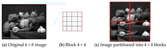
Figure 1.
Example of a 6 × 8 image partitioned into 4 × 4 blocks.
The image in the example is partitioned into four 4 × 4 blocks. Since the number of rows, which is 4, in the blocks does not exactly divide the number of rows in the image, 6, the two blocks below have two rows that do not cover the image; in these blocks, the last two rows replicate the previous two rows and are assigned the values of the corresponding pixels.
Formally, let σN be the integer obtained by dividing N by n and let ρN = 0 if N is divisible by n, otherwise ρN = 1. Furthermore, let σM be the integer obtained by dividing M by n and let ρM= 0 if M is divisible by n, otherwise ρM = 1. The number of blocks, nB, is given by the formula:
In the example in Figure 1, we have that σN = 1, ρN = 1, σM = 2, and ρM = 0; then nB = 4.
The pixel values in each block are normalized as [0, 1]; if ih,k is the pixel value in the cell (h,k) of the block, it is normalized by the formula:
Let R1,i and R2,i be the ith blocks of the images I1 and I2. R1,i and R2,i can be treated as two fuzzy relations, and Algorithms 1 and 2 can be executed to find their GEFS and SEFS. Let GEFS1,i and SEFS1,i be the GEFS and SEFS of R1,i, and let GEFS2,i and SEFS2,i be the GEFS and SEFS of R2,i.
For example, the fuzzy relation R in the previous example is obtained by normalizing the 5 × 5 image block in Figure 2 and having 256 grey levels.
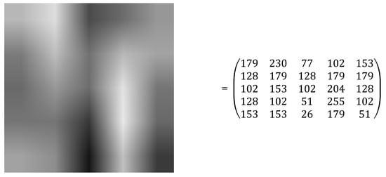
Figure 2.
The 5 × 5 image block normalized in the fuzzy relation R in the previous example.
Following (8), the fuzzy relation R is given by dividing the pixel values in the image block by the value 255.
We measure the distance Di between the two blocks R1,i and R2,i using the Euclidean metric:
The similarity Si between the two ith blocks R1,i and R2,i is given by the following formula:
where the term is the mean distance between two corresponding cells of blocks R1 and R2.
Si varies in the range [0, 1]. It is equal to 1 if and only if the two blocks are equal.
The similarity between the two images is given by the average of the similarity between the corresponding blocks.
Below, in Algorithm 3, the pseudocode of our algorithm used to measure the similarity between the two N × M in images I1 and I2 is shown.
| Algorithm 3: GEFS–SEFS image similarities |
| Input: N × M images I1 and I2 |
| Sizes of the blocks n |
| Output: Similarity S between the two images I1 and I2 |
|
|
4. Discussion and Results
To compare the performances of our method with other IQA similarity measures, an image dataset of over 100 images from the Signal Image Processing Institute (SIPI) image database (https://sipi.usc.edu/database (accessed on 1 February 2023)) was used.
The source image was blurred using a Gaussian filter; the standard deviation σ in the Gaussian distribution increased as the noise increased. We applied our method to measure the similarity between the original and the blurred images by setting n = 5 and afterward n = 7. In addition, we compared our index with the PSNR, SSIM, MS-SSIM, and FSIM indices. For brevity, we show the results obtained for two images: the 256 × 256 image 5.1.09 and the 512 × 512 image 7.1.07.
In Figure 3, the original image 5.01.09 and the blurred images using σ = 0.3, 0.5, 1.0, 1.5, 2.0, 3.0, 4.0, and 5.0, are shown.
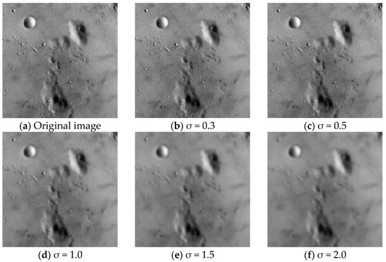
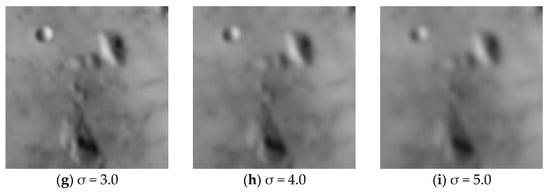
Figure 3.
Image 5.1.09 blurred using Gaussian filters with different values of the parameter σ.
Table 1 shows the similarity indices between the original and the blurred images obtained for image 5.1.09. The PSNR is normalized by dividing its value by the PSNR obtained for σ = 0.3.

Table 1.
Image similarity measures for the grey image 5.1.09.
Therefore, Table 1 shows that the GEFS–SEFS-based similarity indices are more robust to noise than the PSSNR, SSIM, MS-SSIM, and FSIM indices. Indeed, compared to the other indices, the GEFS–SEFS measures do not decrease as quickly as the standard deviation of the Gaussian filter increases. Figure 4 shows the related trends.
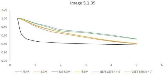
Figure 4.
Similarity index trends for image 5.1.09.
The PSNR decreases quickly starting at σ = 0.5. The SSIM, MS-SSIM, and FSIM decrease below the value of 0.60 starting at σ = 3. Instead, both of the GEFS–SEFS measures obtained for n = 5, 7 slowly decrease and they have no variations, independent of block sizes.
In Figure 5, we show the original image 7.1.07 and the blurred images using σ = 0.3, 0.5, 1.0, 1.5, 2.0, 3.0, 4.0, and 5.0.
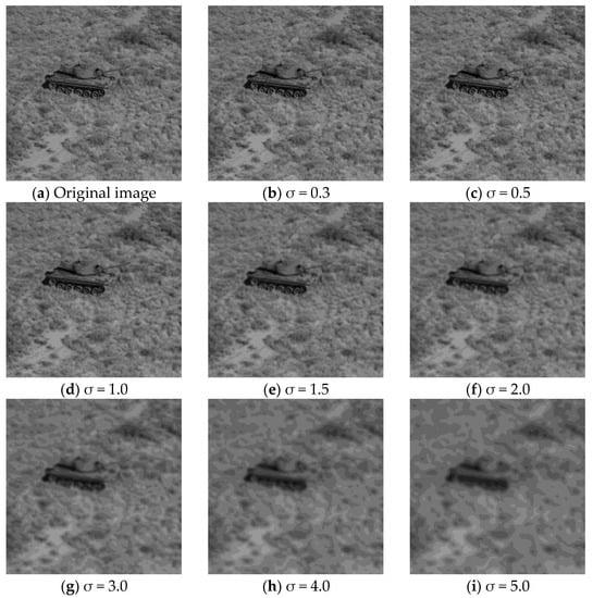
Figure 5.
Image 7.1.07 blurred using Gaussian filters with different values of the parameter σ.
Table 2 shows the similarity indices between the original and the blurred images obtained for image 7.1.07.
Table 2.
Image similarity measures for the grey image 7.1.07.
The GEFS–SEFS measures are more robust to noise than the PSSNR, SSIM, MS-SSIM, and FSIM indices, slowly decreasing with respect to the other image similarity indices. Figure 6 shows the trends for σ varying between 0.3 and 5.
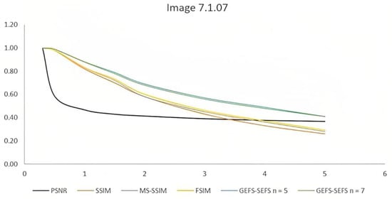
Figure 6.
Similarity indices trends for image 7.1.07.
Figure 6 shows that the trend of the two GEFS–SEFS indices slowly decrease with respect to the similarity indices; moreover, the two GEFS–SEFS measures have the same trend; this confirms that the proposed similarity index is independent of the choice of block sizes. Figure 7 shows the trend of the mean values of the similarity indices obtained for all the images.
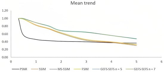
Figure 7.
Mean similarity index trends.
The mean trends show a trend similar to the ones obtained for the two images 5.1.09 and 7.1.07. The two SEFS–GEFS indices obtained by setting n = 5 and n = 7 slowly decrease as soon as the Gaussian noise increases in the image.
These results show, in general, that the GEFS and SEFS-based image similarity measures perform better than the PSNR and SSIM-based measures and that they can be used even in the presence of noise in the images, whereas the performance of the PSNR and SSIM measures decrease quickly.
5. Conclusions
In this paper, we present new image similarity metrics based on the GEFS and SEFS of fuzzy relations; each of the two images to be compared is partitioned in squared blocks, normalized, and treated as squared fuzzy relations. For each block, the GEFS and SEFS are found and the Euclidean distance between the GEFS and SEFS of the corresponding blocks is used to compute the similarity index between the two images. This measure does not require particular parameters to be set beforehand; moreover, the algorithm is computationally fast due to the rapid convergence of the extraction methods of the SEFS and GEFS. The results of the comparative tests carried out on a sample of more than 100 images show that the GEFS–SEFS-based image similarity measure is more efficient and robust to noise than the PSNR and SSIM-based measures.
A critical point of the similarity measure metrics based on the GEFS and SEFS of fuzzy relations is the choice of the size n of the image blocks. In the tests carried out, it was shown that similar results were obtained by setting n = 5 and n = 7, but it is necessary to carry out further tests on a larger sample of images and on different types of problems to analyze if and how the choice of block size affects the performance of this image similarity measure.
In the future, we intend to apply this image similarity to various problems, such as image reconstruction and image tamper detection, and to perform comparative tests by other image similarity measures.
Author Contributions
This article was written in full collaboration by both authors. The final manuscript was read and approved by both authors. All authors have read and agreed to the published version of the manuscript.
Funding
This research received no external funding.
Data Availability Statement
On request, the data used to support the findings of this study can be obtained from the corresponding author.
Conflicts of Interest
The authors declare no conflict of interest.
References
- Wang, Z.; Bovik, A.C. Modern Image Quality Assessment. Synth. Lect. Image Video Multimed. Process. 2006, 2, 1–156. [Google Scholar] [CrossRef]
- Wang, Z.; Bovik, A.C.; Sheikh, H.R.; Simoncelli, E.P. Image Quality Assessment: From Error Visibility to Structural Similarity. IEEE Trans. Image Process. 2004, 13, 600–612. [Google Scholar] [CrossRef] [PubMed]
- Wang, Z.; Simoncelli, E.P.; Bovik, A.C. Multiscale structural similarity for image quality assessment. In Proceedings of the Thrity-Seventh Asilomar Conference on Signals, Systems & Computers, Pacific Grove, CA, USA, 9–12 November 2003. [Google Scholar] [CrossRef]
- Li, C.; Bovik, A.C. Three-component weighted structural similarity index. IS&T/SPIE Electron. Imaging 2009, 7242, 72420Q. [Google Scholar]
- Liu, Z.; Laganière, R. Phase congruence measurement for image similarity assessment. Pattern Recognit. Lett. 2006, 28, 166–172. [Google Scholar] [CrossRef]
- Kovesi, P. Phase congruency: A low-level image invariant. Psychol. Res. 2000, 64, 136–148. [Google Scholar] [CrossRef] [PubMed]
- Chen, G.H.; Yang, C.L.; Xie, S.L. Gradient-based structural similarity for image quality assessment. In Proceedings of the 2006 International Conference on Image Processing, Atlanta, GA, USA, 8–11 October 2006; pp. 2929–2932. [Google Scholar] [CrossRef]
- Han, H.-S.; Kim, D.-O.; Park, R.-H. Gradient information-based image quality metric. IEEE Trans. Consum. Electron. 2010, 56, 361–362. [Google Scholar] [CrossRef]
- Liu, A.; Lin, W.; Narwaria, M. Image Quality Assessment Based on Gradient Similarity. IEEE Trans. Image Process. 2011, 21, 1500–1512. [Google Scholar] [CrossRef] [PubMed]
- Xue, W.; Zhang, L.; Mou, X.; Bovik, A.C. Gradient Magnitude Similarity Deviation: A Highly Efficient Perceptual Image Quality Index. IEEE Trans. Image Process. 2013, 23, 684–695. [Google Scholar] [CrossRef] [PubMed]
- Zhang, L.; Zhang, L.; Mou, X.; Zhang, D. FSIM: A Feature Similarity Index for Image Quality Assessment. IEEE Trans. Image Process. 2011, 20, 2378–2386. [Google Scholar] [CrossRef] [PubMed]
- Sampat, M.P.; Wang, Z.; Gupta, S.; Bovik, A.C.; Markey, M.K. Complex Wavelet Structural Similarity: A New Image Similarity Index. IEEE Trans. Image Process. 2009, 18, 2385–2401. [Google Scholar] [CrossRef] [PubMed]
- Babenko, A.; Slesarev, A.; Chigorin, A.; Lempitsky, V. Neural codes for image retrieval. In Proceedings of the ECCV 2014—13th European Conference, Zurich, Switzerland, 6–12 September 2014. 16 p. [Google Scholar] [CrossRef]
- Melekhov, I.; Kannala, J.; Rahtu, E. Siamese network features for image matching. In Proceedings of the 2016 23rd International Conference on Pattern Recognition (ICPR), Cancun, Mexico, 4–8 December 2016; pp. 378–383. [Google Scholar] [CrossRef]
- Appalaraju, S.; Chaoji, V. Image similarity using Deep CNN and Curriculum Learning. arXiv 2017, arXiv:1709.08761. [Google Scholar] [CrossRef]
- Yuan, X.; Liu, Q.; Long, J.; Hu, L.; Wang, Y. Deep Image Similarity Measurement Based on the Improved Triplet Network with Spatial Pyramid Pooling. Information 2019, 10, 129. [Google Scholar] [CrossRef]
- Ding, K.; Ma, K.; Wang, S.; Simoncelli, E.P. Image Quality Assessment: Unifying Structure and Texture Similarity. IEEE Trans. Pattern Anal. Mach. Intell. 2020, 44, 2567–2581. [Google Scholar] [CrossRef] [PubMed]
- Shanmugamani, R. Deep Learning for Computer Vision: Expert Techniques to Train Advanced Neural Networks Using Ten-sorFlow and Keras; Packt Publishing Ltd.: Birmingham, UK, 2018; 3010 p, ISBN 978-1-78829-562-8. [Google Scholar]
- Felix, R.; Kretzberg, T.; Wehner, M. Image Analysis based on Fuzzy Similarities. In Fuzzy-Systems in Computer Science; Springer: Berlin/Heidelberg, Germany, 1994; pp. 109–116. [Google Scholar] [CrossRef]
- Nachtegael, M.; Schulte, S.; De Witte, V.; Mélange, T.; Kerre, E.E. Image Similarity—From Fuzzy Sets to Color Image Applications. In Advances in Visual Information Systems: 9th International Conference, VISUAL 2007 Shanghai, China, June 28–29, 2007 Revised Selected Papers 9; Springer: Berlin/Heidelberg, Germany, 2007; Volume 4781, pp. 26–37. [Google Scholar] [CrossRef]
- Di Martino, F.; Sessa, S. Comparison between images via bilinear fuzzy relation equations. J. Ambient. Intell. Humaniz. Comput. 2017, 9, 1517–1525. [Google Scholar] [CrossRef]
- Sanchez, E. Resolution of Eigen fuzzy sets equations. Fuzzy Sets Syst. 1978, 1, 69–74. [Google Scholar] [CrossRef]
- Sanchez, E. Eigen fuzzy sets and fuzzy relations. J. Math. Anal. Appl. 1981, 81, 399–421. [Google Scholar] [CrossRef]
- Bourke, M.M.; Fisher, D. Convergence, eigen fuzzy sets and stability analysis of relational matrices. Fuzzy Sets Syst. 1996, 81, 227–234. [Google Scholar] [CrossRef]
- Nobuhara, H.; Hirota, K. A solution for eigen fuzzy sets of adjoint max-min composition and its application to image analysis. In Proceedings of the IEEE International Symposium on Intelligent Signal Processing, Budapest, Hungary, 6 September 2003. [Google Scholar] [CrossRef]
- Di Martino, F.; Nobuhara, H.; Sessa, S. Eigen fuzzy sets and image information retrieval. In Proceedings of the 2004 IEEE International Conference on Fuzzy Systems, Budapest, Hungary, 25–29 July 2004; pp. 1285–1390. [Google Scholar] [CrossRef]
- Di Martino, F.; Sessa, S.; Nobuhara, H. Eigen fuzzy sets and image information retrieval. In Handbook of Granular Computing; Pedrycz, W., Skowron, A., Kreinovich, V., Eds.; Wiley: New York, NY, USA, 2008; pp. 863–872. [Google Scholar] [CrossRef]
- Nobuhara, H.; Bede, B.; Hirota, K. On various eigen fuzzy sets and their application to image reconstruction. Inf. Sci. 2006, 176, 2988–3010. [Google Scholar] [CrossRef]
- Di Martino, F.; Sessa, S. A Genetic Algorithm Based on Eigen Fuzzy Sets for Image Reconstruction. In Applications of Fuzzy Sets Theory: 7th International Workshop on Fuzzy Logic and Applications, WILF 2007, Camogli, Italy, July 7–10, 2007. Proceedings 7; Springer: Berlin/Heidelberg, Germany, 2007; Volume 4578, pp. 342–348. [Google Scholar]
- Rakus-Andersson, E. The greatest and the least eigen fuzzy sets in evaluation of the drug effectiveness levels. In Artificial Intelligence and Soft Computing—ICAISC 2006; Lecture Notes in Computer Science; Rutkowski, L., Tadeusiewicz, R., Zadeh, L.A., Żurada, J.M., Eds.; Springer: Berlin/Heidelberg, Germany, 2006; Volume 402. [Google Scholar]
- Di Martino, F.; Sessa, S. Eigen Fuzzy Sets and their Application to Evaluate the Effectiveness of Actions in Decision Problems. Mathematics 2020, 8, 1999. [Google Scholar] [CrossRef]
- Di Martino, F.; Sessa, S. Image Matching by Using Fuzzy Transforms. Adv. Fuzzy Syst. 2013, 2013, 760704. [Google Scholar] [CrossRef]
Disclaimer/Publisher’s Note: The statements, opinions and data contained in all publications are solely those of the individual author(s) and contributor(s) and not of MDPI and/or the editor(s). MDPI and/or the editor(s) disclaim responsibility for any injury to people or property resulting from any ideas, methods, instructions or products referred to in the content. |
© 2023 by the authors. Licensee MDPI, Basel, Switzerland. This article is an open access article distributed under the terms and conditions of the Creative Commons Attribution (CC BY) license (https://creativecommons.org/licenses/by/4.0/).