Article

Calibration Experiment and Temperature Compensation Method for the Thermal Output of Electrical Resistance Strain Gauges in Health Monitoring of Structures

1
Department of Civil Engineering, University of Science and Technology Beijing, Beijing 100083, China
2
Shunde Innovation School, University of Science and Technology Beijing, Foshan 528399, China
*
Author to whom correspondence should be addressed.
Symmetry 2023, 15(5), 1066; https://doi.org/10.3390/sym15051066
Submission received: 3 April 2023 / Revised: 27 April 2023 / Accepted: 9 May 2023 / Published: 11 May 2023
(This article belongs to the Section Engineering and Materials)

Abstract

:
Electrical resistance strain gauges are widely used in asymmetric structures for measurement and monitoring, but their thermal output in changing temperature environments has a significant impact on the measurement results. Since thermal output is related to the coefficient of thermal expansion of the strain gauge’s sensitive grating material and the measured object, the temperature self-compensation technique of strain gauges fails to eliminate the additional strain caused by temperature because it cannot match the coefficient of thermal expansion of various measured objects. To address this problem, in this study, the principle of the thermal output of electrical resistance strain gauges was analyzed, a calibration experiment for thermal output in the case of a mismatch between the coefficient of linear expansion of the measured object and the strain gauge grating material was conducted, and the mechanism for temperature influence on thermal output was revealed. A method was proposed to obtain the thermal output curves for different materials by using thermostats with dual temperatures to conduct temperature calibration experiments. A linear regression method was used to obtain a linear formula for the thermal output corresponding to each temperature. The thermal output conversion relationship was derived for materials with different coefficients of linear expansion. An in situ temperature compensation technique for electrical resistance strain gauges that separates the measured strain into thermal and mechanical strains was proposed. The results showed that the thermal output curve for the measured object can be calibrated in advance and then deducted from the measured strain, thus reducing the influence of temperature-induced additional strain on the mechanical strain. In addition, a new method was provided for the calculation of the thermal output among materials with similar coefficients of linear expansion, providing a reference for the health monitoring of asymmetric structures.

1. Introduction

Electrical resistance strain gauges have been a key sensing element for structural deformation monitoring, vibration measurement and health diagnosis due to their simple measurement principle and high reliability; these devices have been widely used in mechanical and civil engineering [1,2,3,4,5,6,7]. Ideally, the strain gauges affixed to the measured object respond only to changes in the applied mechanical load and are not affected by environmental conditions. In reality, both the strain gauges and the measured objects deform due to temperature change, resulting in temperature effects, especially for structures with long-term cyclic temperature changes, such as bridges. If these temperature effects are not controlled or eliminated, especially over large temperature ranges, then the thermal output error may completely mask the true measured value. Therefore, it is necessary to use reasonable and effective temperature compensation measures to eliminate their effects [8,9,10,11].
In general, when a strain gauge is mounted on an unrestrained object without any external load, its resistance value also changes if the ambient temperature changes, and this change is referred to as thermal output or apparent strain [12,13,14,15]. The thermal output is the result of the combined action and iterative effect of the difference in the coefficient of linear expansion between the strain gauge’s sensitive grating material and the measured object [16]. Although the strain gauge has the function of temperature self-compensation, when the linear expansion coefficient of the measured object matched by the strain gauge is different from that of the actual measured object, the sensitive grating material will also be subjected to additional tension or compression, resulting in changes in resistance. Since the same strain gauges installed on different materials will have different thermal outputs, the user needs to calibrate the thermal output under actual installation conditions. However, because it takes more time, the thermal output curve of a specific material provided by commercial strain gauge manufacturers is often used directly for temperature compensation in the actual test, but these data only provide meaningful results if the coefficient of thermal expansion of the measured object matches that of the strain gauges; otherwise, they will produce large errors, and this is often ignored by the user.
The effect of thermal output on strain measurements has been explored by many researchers [17,18,19,20]. Various methods have been proposed to eliminate the effect of temperature. Neild et al. [21] conducted theoretical calculations to express the relationship between the measurements and the thermal deformation of a test specimen. These researchers argued that an unstrained strain gauge (i.e., free from structural material deformations but under the same environmental conditions as the test specimen) should be used as a dummy gauge to compensate for the temperature effect. Chen et al. [22,23] used statistical methods, such as linear regression, to investigate the impact of temperature on strain measurements. Litos et al. [24] determined the real strain and thermal output during strain monitoring by using a computer modelling technique. Kieffer et al. [25], from the perspective of strain gauge material composition, demonstrated that the magnitude of the thermal output corresponds with the transformation of the crystalline structure from a state of disorder to a state of order, and the high thermal output can be cancelled by a Wheatstone bridge. Xiao et al. [26] investigated factors influencing the thermal strain measurements of fiber Bragg grating strain sensors and electrical resistance strain gauges through a series of calibration experiments. They proposed a correction method that reduced the relative difference between the strain readings of bonded electrical resistance strain gauges and fiber Bragg grating strain sensors from 82.6% to around 10–20%. Gomes et al. [27] analyzed the thermal output from two different strain gauge types over a temperature range from 20–500 °C; the strain gauges were attached to the specimens in three different configurations. Their results showed that the thermal output was efficiently compensated for using a quarter-bridge configuration. Numerous researchers have conducted cross-corrections and comparisons of the strain measurement of multiple sensors in an environment with changing temperature [28,29,30]. However, because the coupling effect of the strain gauge and the measured object on the thermal output is rarely considered when there is a difference in the coefficient of linear expansion of the strain gauge and the measured object, these thermal strain errors cannot be compensated by a reference strain gauge or virtual temperature fiber, as is usually the case in the Wheatstone bridge measuring circuit [31].
The purpose of this study was to provide a new compensation method for the thermal output of different measured objects and an estimation method for the thermal output between two materials with similar coefficients of thermal expansion. By deriving the calculation equation for the thermal output, the mechanical strain and thermal strain were separated, and the principles of thermal output and temperature self-compensation were analyzed. Temperature calibration tests of various materials were carried out to obtain the thermal output curves applicable to strain gauges affixed to different materials. The results showed that the thermal output and temperature show a linear relationship, and the compensation value of the thermal output at each temperature can be calculated by using the linear formula of the thermal output. When the linear expansion coefficient of the measured object is larger or much smaller than that of the strain gauge grating material, the two thermal output curves exhibit opposite trends. The thermal output conversion relationship was derived for materials with different coefficients of linear expansion. The thermal output of material B can be estimated based on the thermal output of material A and the coefficients of linear expansion of materials A and B. The above established temperature compensation method for strain measurement can effectively reduce the effect of temperature change on mechanical strain to improve the accuracy of strain measurements.

2. Principle of Thermal Output of Electrical Resistance Strain Gauges

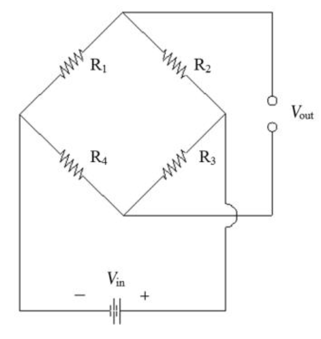
2.1. Measurement Principle of Electrical Resistance Strain Gauges

This resistance change with deformation is called the resistance strain effect. Within a certain range, the relative change in resistance of the sensitive grating material (change rate of resistance: ΔR/R) and the relative change in its length (strain) are linearly related, which can be expressed by Equation (1):
Δ R R = k ε ,
where R is the initial resistance of the strain gauge sensitive grating material with length L ; Δ R is the resistance change of the strain gauge sensitive grating material after elongation Δ L ; ε = Δ L / L is the strain; k is the resistance change per unit of strain, that is, the sensitivity coefficient of the strain gauge.
From Equation (1), the strain value can be found by measuring the change in resistance, which can be measured by a Wheatstone bridge, the measurement principle of which is shown in Figure 1.
The relationship between the output voltage V out and input voltage V in is as follows:
V out = ( R 1 R 3 R 2 R 4 ) ( R 1 + R 2 ) ( R 3 + R 4 ) V in ,
where R 1 , R 2 , R 3 , R 4 are the resistance values.
When R 1 R 3 = R 2 R 4 and V out = 0 , the bridge arms are in equilibrium. When the resistance changes to produce Δ R 1 , Δ R 2 , Δ R 3 , Δ R 4 , respectively, V out is expressed by Equation (3):
V out = ( R 1 + Δ R 1 ) ( R 3 + Δ R 3 ) ( R 2 + Δ R 2 ) ( R 4 + Δ R 4 ) ( R 1 + Δ R 1 + R 2 + Δ R 2 ) ( R 3 + Δ R 3 + R 4 + Δ R 4 ) V in ,
Omitting the term Δ R 2 , we obtain Equation (4):
V out = r V in ( 1 + r ) 2 ( Δ R 1 R 1 Δ R 2 R 2 + Δ R 3 R 3 Δ R 4 R 4 ) ,
where r = R 1 R 2 = R 4 R 3 , and when r = 1 , Equation (4) becomes
V out = V in 4 ( Δ R 1 R 1 Δ R 2 R 2 + Δ R 3 R 3 Δ R 4 R 4 ) ,
In conventional bridges, R 1 = R 2 = R 3 = R 4 is adopted.
V out = V in 4 ( Δ R 1 Δ R 2 + Δ R 3 Δ R 4 R ) ,
If the strain gauge is connected to four bridge arms, it is called a full bridge line; if only two bridge arms are connected, (e.g., R 1 and R 2 ), it is called a half bridge line; if only one bridge arm is connected (e.g., R 1 ), it is called a quarter bridge line.
During the measurement, if only the resistance strain gauge (working gauge) is in working condition, its resistance will change; the resistance of the other three bridge arms is not changed, so Equation (6) becomes
V out = V in 4 Δ R 1 R ,
where R 1 and Δ R 1 are the initial resistance value and the change in resistance value of the resistance strain gauge, respectively.
Substituting Equation (1) into Equation (7), we obtain
ε = 4 k V out V in ,
Since k and V in are known, the strain value can be found from the output voltage of the bridge arms, which is the principle of strain measurement using Wheatstone bridges.
In the actual measurement, if we make V in = 4 k , then Equation (8) becomes
ε = V out ,
That is, the voltage output from the bridge arms is the strain value. Usually, the voltage in the bridge arms is V in = 2 v , and the sensitivity coefficient of the strain gauge is k = 2 .

2.2. Coupled Thermo-Electro-Elasticity Equations

Due to the physical properties of the sensitive grating materials used to make strain gauges, even if the strain gauges are mounted on a specimen without any external forces, the resistance value changes when the ambient temperature changes; this is called the temperature effect. When the measured specimen is subjected to both load and temperature, the output value of the strain gauge is not only related to the deformation of the measured specimen but also to the temperature, that is, the resistance change of the strain gauge is a function of temperature ( T ) and strain ( ε ), which can be expressed by Equation (10):
R = f ( T , ε ) ,
The change in resistance of a strain gauge can be expressed by the partial differential Equation (11):
Δ R = R T Δ T + R ε Δ ε ,
The rate of change in resistance can be expressed by Equation (12):
Δ R R = R R · T Δ T + R R · ε Δ ε ,
{ R R · T = α R R R · ε = k ,
where T is the temperature; Δ T is the temperature change; Δ ε is the strain change; and α R is the temperature coefficient of the strain gauge’s sensitive grating material.
The rate of change in resistance can be expressed by Equation (14):
Δ R R = k Δ ε + α R Δ T ,
Since the strain gauges are affixed to the measured specimens and need to deform together under the action of temperature, their strain change Δ ε is composed of the strain of the measured specimens ( Δ ε s ) and the strain of the sensitive grating material ( Δ ε g ), i.e.,
Δ ε = Δ ε g + Δ ε s ,
When the coefficient of linear expansion of the sensitive grating material ( α g ) differs from that of the measured specimen ( α s ), i.e., α s α g , the additional strain on the strain gauge is the difference between these coefficients when the measured specimen is free to expand and contract, as expressed by Equation (16),
Δ ε g = ( α s α g ) Δ T ,
Substituting Equation (16) into Equation (15) gives Equation (17):
Δ ε = ( α s α g ) Δ T + Δ ε s ,
Substituting Equation (17) into Equation (14) gives Equation (18):
Δ R R = k [ ( α s α g ) Δ T + Δ ε s ] + α R Δ T ,
When no load is applied to the measured object, Δ ε s = 0 ; the output values of the strains are all thermal strains, and Equation (18) becomes
Δ R R = k ( α s α g ) Δ T + α R Δ T = k Δ ε T ,
Namely:
Δ ε T = α R Δ T k + ( α s α g ) Δ T ,
where Δ ε T is the thermal output of the strain gauge; α s is the coefficient of linear expansion of the measured material; and α g is the coefficient of linear expansion of the strain gauge’s sensitive grating material.
Equation (20) gives the effect of temperature on the strain gauges. The reason for the thermal output is mainly due to the difference between the coefficient of linear expansion of the sensitive grating material and that of the measured material.
According to Equation (20), we are able to change the parameters of strain gauges by some measures so that the thermal output of each strain gauge is zero or fluctuates within a specified range. This is the basic principle of the self-compensation technology for strain gauges. It can be expressed as Equation (21):
Δ ε T = α R Δ T k + ( α s α g ) Δ T = 0 ,
Equation (22) can be obtained from Equation (21):
α R = k ( α g α s ) ,
From Equation (22), it can be seen that the temperature coefficient α R and the coefficient of linear expansion α g can be adjusted to satisfy Equation (22) by controlling the alloy composition of the strain gauge sensitive grating material and the heat treatment process. Thus, the temperature self-compensation function for the specific measured object is realized. Ideally, the thermal output value for such strain gauges tends to zero, and these strain gauges are called temperature self-compensated strain gauges.
This basic principle shows that the self-compensating strain gauge must correspond to the coefficient of linear expansion for the specific measured material. If the measured material does not match the one corresponding to that of the self-compensating strain gauge, then effective temperature compensation cannot be achieved. In this case, it is necessary to obtain the thermal output curve of the strain gauge for the actual conditions instead of the thermal output curve provided by the manufacturer, which leads to large measurement errors. Furthermore, a constant coefficient of linear expansion is required for self-compensating technology, but in some cases, the temperature difference varies greatly so that the coefficient of thermal expansion is not constant.

2.3. Elastic Constitutive Relation

In a perfectly elastic isotropic body, it follows from Hooke’s law that
ε x = 1 E [ σ x ν ( σ y + σ z ) ] ε y = 1 E [ σ y ν ( σ x + σ z ) ] ε z = 1 E [ σ z ν ( σ x + σ y ) ] } ,
where E is the modulus of elasticity, ν is Poisson’s ratio, ε x , ε y , ε z are the strain components in the directions of x , y , z , respectively; σ x , σ y , σ z are the stress components in the directions of x , y , z , respectively.
In Section 2.1, the measured resistance is the change in resistance, i.e., the change in strain, so Equation (23) is written in incremental form, and substituting Equation (9) into Equation (23) gives
Δ V out , x = 1 E [ Δ σ x ν ( Δ σ y + Δ σ z ) ] Δ V out , y = 1 E [ Δ σ y ν ( Δ σ x + Δ σ z ) ] Δ V out , z = 1 E [ Δ σ z ν ( Δ σ x + Δ σ y ) ] } ,
where Δ V out , x , Δ V out , y , Δ V out , z are the output value of voltage in the directions of x , y , z , respectively.
Equation (24) comprises coupled electro-elasticity equations.
Since resistance strain gauges are very sensitive to temperature changes, their resistance values change when the temperature changes. As shown in Equation (9), this change in resistance generates an output voltage, which is reflected in a strain value. However, this part of the strain value is not caused by the change in stress, but by the change in temperature, so it is an additional strain value. Therefore, the total output value in the Wheatstone bridge consists of the thermal and mechanical outputs of the strain gauge,
Δ ε total = Δ ε + Δ ε T ,
where Δ ε total is the total output value of the strain gauge, Δ ε is the mechanical output of the strain value, and Δ ε T is the thermal output of the strain value.
Substitute Equations (20) and (23) into Equation (25), where the strain output in the direction of x is expressed as
Δ ε total = 1 E [ Δ σ x ν ( Δ σ y + Δ σ z ) ] + α R Δ T k + ( α s α g ) Δ T ,
Substitute Equation (9) into (26) and write it in incremental form:
Δ V out , total = 1 E [ Δ σ x ν ( Δ σ y + Δ σ z ) ] + α R Δ T k + ( α s α g ) Δ T ,
where Δ V out , total is the change in total voltage output.
Equation(27) is a coupled thermo-electro-elasticity equation.
If no compensation measures are applied, then the thermal output is present in the output value. If the strain gauge is attached to the measured object and placed in the test environment before the official test, then the strain output value without mechanical load is the thermal output of the gauge itself. Regardless of whether α R , α s and α g are constants or not, or regardless of the type of measured object, this thermal output can be deducted from the measured strain to obtain an accurate mechanical strain.

3. Temperature Calibration Experiments for Different Measured Materials

3.1. Zero-Drift Experiment

After a strain gauge is attached to the surface of an object in a no-load and constant temperature environment, the change in the indicated strain over time is called the “zero drift” of the electrical resistance strain gauge. This parameter is related to the strain gauge grating material, the bonding and curing process, the welding of lead wires, the measurement environment, the power supply voltage, etc., and is the stability parameter of the strain gauge itself, expressed as με/H.
It is necessary to test the “zero drift” performance to determine the stability of the strain gauge. In this work, the strain gauge and the logging system were placed in a constant ambient temperature, and the data were recoded directly every 15 min for a total of 48 h without applying a mechanical load (free strain gauge). The maximum fluctuation within 1 h was used as the “zero drift” value for the temperature, and the test results are shown in Figure 2. The minimum value of strain was −29 με, and the maximum value was 38 με. Specifically, the maximum fluctuation was 67 με within 48 h. The maximum fluctuation within 1 h was 8 με, i.e., 8 με/H. Therefore, this “zero drift” range is acceptable in practical measurements.

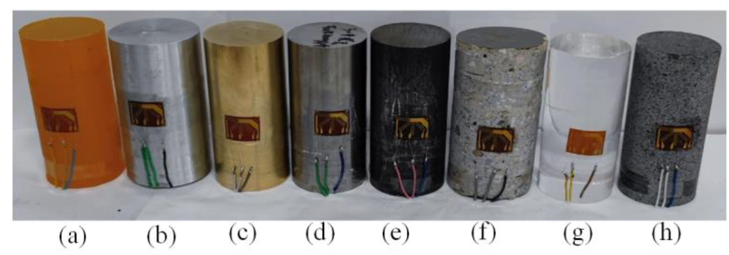
3.2. Calibration Experiments for the Thermal Output of Different Measured Materials

From Equation (20), the thermal output of a strain gauge is related to the coefficient of linear expansion of the measured object in addition to its own temperature coefficient and coefficient of linear expansion. Therefore, the method using a dummy strain gauge placed in the compensation channel of the logging system can cause significant errors during long-term monitoring with large temperature variations or when the coefficient of linear expansion of the measured material differs significantly from that of the strain gauge grating material. It is necessary to consider the influence of various factors, such as the type of binder, the thickness of the binder, and the measured material, to reduce the influence of the thermal output of the strain test system. Corresponding indoor calibration tests are required to obtain the thermal output of strain gauges under the influence of temperature, and then error elimination can be performed based on temperature variations during long-term monitoring.
A variety of materials with different coefficients of linear expansion commonly used in civil engineering (epoxy resin adhesive, metal, plexiglass, concrete and rock) were selected to carry out the calibration experiment for the thermal output of strain gauges, as shown in Figure 3. The relationship between the coefficients of linear expansion of the different materials is as follows: epoxy resin adhesive > strain gauge grating material > aluminum > brass > stainless steel > iron > concrete > plexiglass > granite. Electrical resistance strain gauges with temperature self-compensation were used. The temperature coefficient of the strain gauges was 30 με/°C, and their sensitivity coefficient was 2.18; the coefficient of linear expansion was 25.1 × 10⁻⁶/°C. The test specimen with strain gauges attached was put into high- and low-temperature test thermostats (as shown in Figure 4a), a free strain gauge was set for comparison, and the logging system was in a test thermostat with a constant temperature (keeping the temperature constant at 30 °C), as shown in Figure 4b. The temperature gradient was set to 10 °C, 20 °C, 30 °C, 40 °C and 50 °C, and each temperature gradient lasted for 8 h with a record interval of 15 min. The test results are shown in Figure 5.
According to the results, under the condition of 10~50 °C, the thermal output of the strain gauge in the free state was approximately 1295 με. The thermal output of the strain gauges pasted with the epoxy resin adhesive was 5711 με, which was larger than that in the free state. This is because the coefficient of linear expansion of the epoxy resin material (56.8 × 10⁻⁶/°C) was larger than that of the strain gauge grating material (25.1 × 10⁻⁶/°C). The thermal outputs of the strain gauges pasted on aluminum, brass and stainless steel were 778 με, 622 με and 400 με, respectively, which were all smaller than the thermal output in the free state. This is because the coefficients of linear expansion of the three materials were smaller than that of the strain gauge grating material. The thermal output of the strain gauges pasted on iron showed a nonlinear variation with temperature, and the thermal output was close to zero because the coefficient of linear expansion of iron almost satisfied Equation (22) and thus produced a temperature self-compensation effect. The thermal output of the above materials showed positive values in the test channel. The thermal outputs of concrete, plexiglass and granite were −166 με, −214 με and −352 με, respectively, which were much smaller than the thermal output in the free state. Their coefficients of linear expansion were much smaller than those of the strain gauge grating materials, making ε T = α R Δ T k + ( α s α g ) Δ T < 0 . This means that these materials constrained the deformation of the strain gauges, which is shown as a negative value in the test channel, and the thermal output curves show opposite trends corresponding to positive values. The greater the difference in the coefficient of linear expansion of the different materials is, the greater the thermal output, and therefore, it is inappropriate to use the method of placing a free strain gauge to offset the additional strain caused by temperature. If conditions allow, then it is more appropriate to attach a strain gauge to the measured object (the same measured material, the same temperature environment, kept unconstrained) as a compensation block during the measurement to offset the temperature effect.
In summary, when the coefficient of linear expansion of the measured material is larger or much smaller than that of the strain gauge grating material, the two types of thermal output curves will show opposite trends: one is an upward trend (positive thermal output) and the other is a downward trend (negative thermal output). The relationship between α s and α g in Equation (22) can explain this phenomenon well. This means that when the coefficient of linear expansion of the measured material is larger than that of the strain gauge grating material during a temperature change, strain gauge elongation is promoted. When the coefficient of linear expansion of the measured material is smaller than that of the strain gauge grating material, strain gauge elongation is prevented. This may be slightly difficult to understand, so we provide a detailed explanation in the subsequent subsections.

3.3. Calculation of the Thermal Output for Different Measured Materials

The middle value of the thermal output curve at each temperature gradient is taken as the representative value of the thermal output at this temperature, as shown in Table 1. The fitting line of the thermal output for each material can be obtained by the linear fitting method, and the results are shown in Figure 6. Except for iron, the relationship between the thermal output and temperature change in various materials shows a linear trend. The coefficient of linear expansion of iron matches that of the strain gauge grating material; thus, the strain gauges fulfill a temperature self-compensation function, as in Equation (14), and the thermal output is almost zero. The corresponding thermal output at each temperature can be calculated from the fitting line of the thermal output and the actual temperature during the measurement, and then the additional strain caused by temperature is deducted from the strain measurement results to obtain an accurate strain induced by mechanics, as in Equation (25).

3.4. Coupled Deformation Analysis of Strain Gauges and Measured Materials

When the coefficient of linear expansion of the measured object is smaller or much smaller than that of the strain gauges, under the reference temperature (such as 10 °C), the initial length of the free strain gauge and the measured object are assumed to be L0, as shown in Figure 7a. However, after the temperature increases (such as 50 °C), if the strain gauge is in a free state (the strain gauge and the measured object are separated), then its length change should be ΔL, and the length change in the measured object should be ΔL1. However, when the strain gauge is attached to the measured object (the strain gauge and the measured object are coupled), the strain gauge has the same deformation as the measured material due to the constraint action of the measured material, so the length change in the strain gauge after the temperature increase is only ΔL1. That is, it is equivalent to a shrinkage of the strain gauge by ΔL2 compared to the free strain gauge. Therefore, the thermal output of the strain gauge is smaller or negatively increased (the opposite direction of deformation from the free state).
When the coefficient of linear expansion of the measured object is greater than that of the strain gauge, under the reference temperature condition (such as 10 °C), the initial lengths of the free strain gauge and the measured object are assumed to be L0, as shown in Figure 7b. However, after the temperature increases (such as 50 °C), if the strain gauge is in a free state, then its length change should be ΔL, and the length change in the measured object should be (ΔL + ΔL1). However, when the strain gauge is attached to the measured object, the strain gauge has the same deformation as the measured material due to the constraint action of the measured material, so the length change in the strain gauge after the temperature increase is (ΔL + ΔL1) instead of ΔL. That is, it is equivalent to elongation of the strain gauge by ΔL1 compared to the free strain gauge, so the thermal output of the strain gauge is greater or positively increased (greater than free state). This is the fundamental reason why strain gauges have different thermal outputs when attached to different materials.

3.5. Analysis of the Error Caused by the Thickness of an Adhesive Layer

In general, strain gauges are coupled to a measured object through a bonded adhesive layer, but the thickness of the adhesive layer is generally controlled manually, and the coefficient of linear expansion of different types of adhered materials varies widely. This can have an effect on the thermal output. In addition, sometimes the strain gauges are not directly bonded to one material but to multiple composite materials, in which case the strain gauges are subject to the coupling effects of multiple materials. For example, in the CSIRO method for in situ stress measurements, developed by our research team [32], strain gauges were pasted on a composite of adhesive layer and rock, where the thickness of the adhesive layer had an effect on the thermal output.
Therefore, five sets of calibration tests were conducted for strain gauges pasted under adhesive layers with different thicknesses. The adhesive material was epoxy resin adhesive, and its thicknesses were 0 (as a comparison), 0.5 mm, 1 mm, 2 mm, 3 mm, 4 mm and 5 mm, as shown in Figure 8. The temperature gradients were set to 10 °C, 20 °C, 30 °C, 40 °C and 50 °C, and the test results are shown in Figure 9.
The results showed that the thermal output of the strain gauges increased significantly when the bond thickness was in the range of 0.5 to 2 mm relative to that of the strain gauges pasted on the rocks. In addition, the increase in the thermal output of the strain gauges was no longer significant when the bond thickness reached 2 mm, at which time the thermal output of the strain gauges was mainly determined by the coefficient of linear expansion of the epoxy resin adhesive, and the constraint effect of the rocks decreased significantly. Within 20 °C, this difference was relatively small, while with increasing temperature, this difference became increasingly larger. Therefore, the thickness of the adhesive layer between the strain gauges and the measured object, as well as the thickness of the outer adhesive layer of the composite material, should be reduced as much as possible when pasting strain gauges to reduce the influence of the thermal output, especially under high temperature conditions.

4. Conversion Relationship of Strain Gauge Thermal Output for Different Materials

4.1. Calculation Principle

The strain gauge self-compensation technique can be a good method to address the thermal output in some strain measurements of specific materials. This allows the manufacturer to develop specific strain gauges to reduce the thermal output based on the temperature characteristics of the strain gauge grating material and the thermal expansion characteristics of the measured material. However, in general, the user’s test material does not match the manufacturer’s specific application, making the self-compensation technique ineffective.
To obtain the thermal output curves for strain gauges on various objects, the strain gauges must first be attached to the corresponding measured objects and then tested in temperature thermostats, which usually takes a long time. Fortunately, among civil engineering materials, some materials have similar thermal expansion characteristics. In some practical applications, sometimes when the thermal output of the strain gauge on material A is known and the thermal output of the strain gauge on material B needs to be obtained as soon as possible, a simple calculation method can be used to rapidly obtain that of the strain gauge on material B. The basic principle is as follows:
The thermal output of the strain gauge on specimen material A can be expressed as:
ε T A = α R Δ T k + ( α s A α g ) Δ T ,
Similarly, the thermal output of the strain gauge on material B can be expressed as:
ε T B = α R Δ T k + ( α s B α g ) Δ T ,
Equations (28) and (29), give the following:
ε T B ε T A = [ α R Δ T k + ( α s B α g ) Δ T ] [ α R Δ T k + ( α s A α g ) Δ T ] = ( α s B α s A ) Δ T ,
After the transformation, we obtain Equation (31):
ε T B = ε T A + ( α s B α s A ) Δ T ,
where ε T A is the thermal output of the strain gauge on material A (known); ε T B is the thermal output of the strain gauge on material B (unknown); α s A and α s B are the coefficients of linear expansion of materials A and B, respectively; and Δ T is the temperature change.
In summary, the thermal output of the strain gauge on material (B) can be obtained from Equation (31).

4.2. Calculation Example

The thermal output data for the strain gauge on specimen A (brass) are known, and the thermal output curve for the strain gauge on specimen B (aluminum) is needed. According to the material manual, the coefficient of linear expansion of brass is 17.1 × 10⁻⁶/°C, and that of aluminum is 22.5 × 10⁻⁶/°C. The following can be obtained from Equation (29): ε T B = ε T A + (22.5 − 17.1) Δ T (με).
The results of the calculations are shown in Table 2. To confirm the reliability of Equation (31), the thermal output was measured by using strain gauges pasted on aluminum material, and the results are shown in Table 2. The maximum difference between the two was within 10% in the range of 10 °C to 50 °C, so the above method is feasible. Notably, the coefficient of thermal expansion tends to be different at different temperature gradients, i.e., nonlinear, so this is only an estimation method for adjacent temperature gradients and materials with similar linear expansion coefficients.

5. Conclusions

In this study, the mechanical strain and thermal strain were separated by deriving a strain gauge thermal output calculation equation. Thermal output calibration experiments for different materials were carried out to provide a thermal output compensation method and a thermal output estimation method between different materials.
(1)
The thermal output curves applicable to different materials were obtained based on temperature calibration tests conducted on a variety of materials. The thermal output shows a linear relationship with temperature, and the thermal output compensation value at each temperature can be calculated according to the thermal output fitting formula.
(2)
When the coefficient of linear expansion of the measured material is larger or much smaller than that of the strain gauge grating material, the two thermal output curves show an opposite trend. This means that when the coefficient of linear expansion of the measured material is larger than that of the strain gauge grating material, the elongation of the strain gauges is promoted, and thus, the thermal output during the temperature change is increased. When the coefficient of linear expansion of the measured material is smaller than that of the strain gauge grating material, the elongation of the strain gauges is prevented, and thus, the thermal output decreases.
(3)
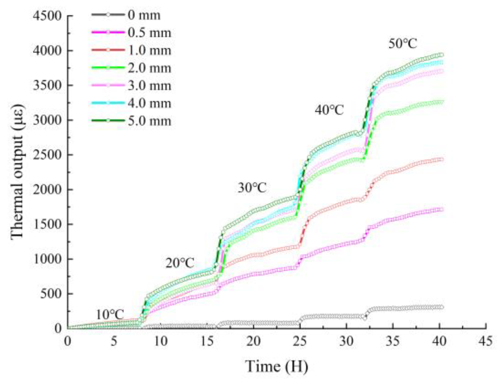
The thickness of the adhesive layer between the strain gauge and the measured object affects the thermal output. The thermal output of the strain gauge increases significantly when the thickness of the adhesive layer is in the range of 0.5 to 2 mm. When the thickness of the adhesive layer reaches 2 mm, the increase in the thermal output of the strain gauge is no longer significant. This difference is relatively small within 20 °C but becomes increasingly larger as the temperature increases.
(4)
The thermal output conversion relationships were derived for materials with different linear expansion coefficients. The thermal output of material B was estimated from the thermal output of material A and the linear expansion coefficients of the two materials (A and B), and the maximum difference between the estimated and actual values was within 10% in the range of 10 °C to 50 °C.

Author Contributions

Data curation, D.F., C.T., X.W. and S.D.; writing—original draft, Z.J.; writing—review and editing, Y.L. All authors have read and agreed to the published version of the manuscript.

Funding

This work was supported by the Foshan Science and Technology Innovation Special Fund Funding Project (Grant No. BK21BE014) and the National Key Research and Development Program of China (Grant No. 2022YFC2904102).

Data Availability Statement

Not applicable.

Conflicts of Interest

The authors declare no conflict of interest.

References

  1. Tegtmeier, F.L. Strain gauge based microsensor for stress analysis in building structures. Measurement 2008, 41, 1144–1151. [Google Scholar] [CrossRef]
  2. Yang, Y. Special Issue Editorial “Symmetry in Structural Health Monitoring”. Symmetry 2022, 14, 1211. [Google Scholar] [CrossRef]
  3. Lei, J.; Kong, Q.; Wang, X.; Zhan, K. Strain Monitoring-Based Fatigue Assessment and Remaining Life Prediction of Stiff Hangers in Highway Arch Bridge. Symmetry 2022, 14, 2501. [Google Scholar] [CrossRef]
  4. Ding, M.; Shen, Y.; Wei, Y.; Luo, B.; Wang, L.; Zhang, N. Preliminary Design and Experimental Study of a Steel-Batten Ribbed Cable Dome. Symmetry 2021, 13, 2136. [Google Scholar] [CrossRef]
  5. Shi, G.; Liu, Z.; Meng, X.; Wang, Z. Intelligent Health Monitoring of Cable Network Structures Based on Fusion of Twin Simulation and Sensory Data. Symmetry 2023, 15, 425. [Google Scholar] [CrossRef]
  6. Wang, T.; Shi, B.; Zhu, Y. Structural Monitoring and Performance Assessment of Shield Tunnels during the Operation Period, Based on Distributed Optical-Fiber Sensors. Symmetry 2019, 11, 940. [Google Scholar] [CrossRef]
  7. Jin, Z.H.; Li, Y.; Li, Q.W.; Liu, Z.B.; Wu, S.B.; Wang, Z. Modification of the CSIRO method in the long-term monitoring of slope-induced stress. Front. Earth Sci. 2022, 10, 981470. [Google Scholar] [CrossRef]
  8. Xia, Y.; Chen, B.; Weng, S.; Ni, Y.Q.; Xu, Y.L. Temperature effect on vibration properties of civil structures: A literature review and case studies. J. Civ. Struct. Health Monit. 2012, 2, 29–46. [Google Scholar] [CrossRef]
  9. Kromanis, R.; Kripakaran, P. SHM of bridges: Characterising thermal response and detecting anomaly events using a temperature-based measurement interpretation approach. J. Civ. Struct. Health Monit. 2016, 6, 237–254. [Google Scholar] [CrossRef]
  10. Liu, X.; Kang, F.; Ma, C.B.; Li, H.J. Concrete arch dam behavior prediction using kernel-extreme learning machines considering thermal effect. J. Civ. Struct. Health Monit. 2021, 11, 283–299. [Google Scholar] [CrossRef]
  11. Zhao, H.W.; Ding, Y.L.; Li, A.Q.; Chen, B.; Wang, K.P. Digital modeling approach of distributional mapping from structural temperature field to temperature-induced strain field for bridges. J. Civ. Struct. Health Monit. 2022, 13, 251–267. [Google Scholar] [CrossRef]
  12. Hoffmann, K. An Introduction to Measurements Using Strain Gages; Hottinger Baldwin Messtechnik GmbH: Darmstadt, Germany, 1989; p. 257. [Google Scholar]
  13. John, N.F. Measurement of thermal expansion coefficients using a strain gauge. Am. J. Phys. 1990, 58, 875. [Google Scholar]
  14. Cappa, P.; Rita, G.D.; McConnell, K.G.; Zachary, L.W. Using strain gages to measure both strain and temperature. Exp. Mech. 1992, 32, 230–233. [Google Scholar] [CrossRef]
  15. Richards, W.L. A new correction technique for strain-gage measurements acquired in transient-temperature environments. In NASA Technical Reports Server (NTRS); Edwards: California, CA, USA, 1996; p. 3593. [Google Scholar]
  16. Batten, M.; Powrie, W.; Boorman, R.; Yu, H.T.; Leiper, Q. Use of vibrating wire strain gauges to measure loads in tubular steel props supporting deep retaining walls. Proc. Inst. Civ. Eng.-Geotech. Eng. 1999, 137, 3–13. [Google Scholar] [CrossRef]
  17. Cappa, P.; Marinozzi, F.; Sciuto, S.A. The “strain-gauge thermocouple”: A novel device for simultaneous strain and temperature measurement. Rev. Sci. Instrum. 2001, 72, 193–197. [Google Scholar] [CrossRef]
  18. Rodrigues, C.; Félix, C.; Lage, A.; Figueiras, J. Development of a long-term monitoring system based on FBG sensors applied to concrete bridges. Eng. Struct. 2010, 32, 1993–2002. [Google Scholar] [CrossRef]
  19. Aiyeh, E. Thermal Output and Thermal Compensation Models for Apparent Strain in a Structural Health Monitoring-Based Environment. Master’s Thesis, University of Manitoba, Winnipeg, Manitoba, 2012. [Google Scholar]
  20. Zhao, Y.; Liu, Y.; Li, Y.; Hao, Q. Development and application of resistance strain force sensors. Sensors 2020, 20, 5826. [Google Scholar] [CrossRef]
  21. Neild, S.A.; Williams, M.S.; McFadden, P.D. Development of a vibrating wire strain gauge for measuring small strains in concrete beams. Strain 2005, 41, 3–9. [Google Scholar] [CrossRef]
  22. Chen, C.; Wang, Z.; Wang, Y.; Wang, T.; Luo, Z. Reliability assessment for PSC box-girder bridges based on SHM strain measurements. J. Sens. 2017, 2017, 8613659. [Google Scholar] [CrossRef]
  23. Prakash, G.; Sadhu, A.; Narasimhan, S.; Brehe, J.M. Initial service life data towards structural health monitoring of a concrete arch dam. Struct. Control Health Monit. 2018, 25, e2036. [Google Scholar] [CrossRef]
  24. Litoš, P.; Švantner, M.; Honner, M. Simulation of strain gauge thermal effects during residual stress hole drilling measurements. J. Strain Anal. Eng. Des. 2005, 40, 611–619. [Google Scholar] [CrossRef]
  25. Kieffer, T.P.; Peters, K.J. The effect of short range order on the thermal output and gage factor of Ni3FeCr strain gages. Strain 2017, 54, e12253. [Google Scholar] [CrossRef]
  26. Xiao, X.; Li, H.X.; Cui, H.Z.; Bao, X.H. Evaluation of thermal-drift effect on strain measurement of energy pile. Constr. Build. Mater. 2023, 362, 129663. [Google Scholar] [CrossRef]
  27. Gomes, P.T.V.; Maia, N.S.; Mansur, T.R.; Palma, E.S. Temperature effect on strain measurement by using weldable electrical resistance strain gages. J. Test. Eval. 2003, 31, 363–369. [Google Scholar]
  28. Yu, G.; Elshafie, M.Z.E.B.; Dirar, S.; Middleton, C.R. The response of embedded strain sensors in concrete beams subjected to thermal loading. Constr. Build. Mater. 2014, 70, 279–290. [Google Scholar] [CrossRef]
  29. Ye, C.; Butler, L.J.; Elshafie, M.Z.E.B.; Middleton, C.R. Evaluating prestress losses in a prestressed concrete girder railway bridge using distributed and discrete fibre optic sensors. Constr. Build. Mater. 2020, 247, 118518. [Google Scholar] [CrossRef]
  30. Clauß, F.; Ahrens, M.A.; Mark, P. A comparative evaluation of strain measurement techniques in reinforced concrete structures–A discussion of assembly, application, and accuracy. Struct. Concr. 2021, 22, 2992–3007. [Google Scholar] [CrossRef]
  31. Mohamad, H. Distributed Optical Fibre Strain Sensing of Geotechnical Structures. Ph.D. Thesis, Universiti Teknologi Petronas, Seri Iskandar, Malaysia, 2008. [Google Scholar]
  32. Li, Y.; Fu, S.S.; Qiao, L.; Liu, Z.B.; Zhang, Y.H. Development of twin temperature compensation and high-level biaxial pressurization calibration techniques for CSIRO in-situ stress measurement in depth. Rock Mech. Rock Eng. 2019, 52, 1115–1131. [Google Scholar] [CrossRef]
Figure 1. Wheatstone bridge circuit.
Symmetry 15 01066 g001
Figure 2. The “zero drift” data for a strain gauge.
Symmetry 15 01066 g002
Figure 3. Strain gauges pasted on measured materials with different linear expansion coefficients: (a) epoxy resin adhesive, (b) aluminum, (c) brass, (d) stainless steel, (e) iron, (f) concrete, (g) plexiglass, and (h) granite.
Symmetry 15 01066 g003
Figure 4. Thermostats with dual temperatures. (a) high- and low-temperature thermostats: −40∼150 °C (±0.1 °C); (b) Ambient temperature thermostats: 15∼50 °C (±0.1 °C).
Symmetry 15 01066 g004
Figure 5. Thermal output of the strain gauges pasted onto different materials: (a) epoxy resin adhesive; (b) free strain gauge, aluminum, brass, stainless steel, iron; (c) concrete, plexiglass, granite.
Symmetry 15 01066 g005
Figure 6. Fitting line of the thermal output of strain gauges pasted onto different measured materials: (a) epoxy resin adhesive; (b) free strain gauge, aluminum, brass, stainless steel, iron; (c) concrete, plexiglass, granite.
Symmetry 15 01066 g006
Figure 7. Coupled deformation of strain gauges and measured materials during temperature change: (a) αs < αg; (b) αs > αg.
Symmetry 15 01066 g007
Figure 8. Strain gauges pasted on adhesive layers with different thicknesses: (a) 0; (b) 0.5 mm; (c) 1.0 mm; (d) 2.0 mm; (e) 3.0 mm; (f) 4.0 mm; (g) 5.0 mm.
Symmetry 15 01066 g008
Figure 9. Relationship of temperature to thermal output for different paste thicknesses of the adhesive layer.
Symmetry 15 01066 g009
Table 1. Thermal output of different materials corresponding to temperature (unit: με).
T/°CEpoxy Resin AdhesiveFree Strain GaugeAluminumBrassStainless SteelIronConcretePlexiglassGranite
10−34−12251510142−7−7
20112824524220213853−14−51−76
30235949743533722771−38−95−156
40463682560749531955−101−156−257
505711129577862240043−166−214−352
Table 2. Estimated thermal output for the strain gauge on material B.
T/°CΔT/°C ε T A ε T B ε T B Relative   Errors :   ( ε T B ε T B ) / ε T B
100////
20102022562425.8%
30203374454352.3%
40304956576078.2%
50406228387787.7%
Disclaimer/Publisher’s Note: The statements, opinions and data contained in all publications are solely those of the individual author(s) and contributor(s) and not of MDPI and/or the editor(s). MDPI and/or the editor(s) disclaim responsibility for any injury to people or property resulting from any ideas, methods, instructions or products referred to in the content.

