Training Data Selection for Record Linkage Classification

Abstract

This paper presents a new two-step approach for record linkage, focusing on the creation of high-quality training data in the first step. The approach employs the unsupervised random forest model as a similarity measure to produce a similarity score vector for record matching. Three constructions were proposed to select non-match pairs for the training data, with both balanced (symmetry) and imbalanced (asymmetry) distributions tested. The top and imbalanced construction was found to be the most effective in producing training data with 100% correct labels. Random forest and support vector machine classification algorithms were compared, and random forest with the top and imbalanced construction produced an F₁-score comparable to probabilistic record linkage using the expectation maximisation algorithm and EpiLink. On average, the proposed approach using random forests and the top and imbalanced construction improved the F₁-score by 1% and recall by 6.45% compared to existing record linkage methods. By emphasising the creation of high-quality training data, this new approach has the potential to improve the accuracy and efficiency of record linkage for a wide range of applications.

1. Introduction

Databases enable entities’ information to be stored in repositories that are dispersed across different computer systems. Occasionally, entity resolution is required to ensure that records from different databases refer to the same real-world entities, which can be a person, a place, an object, or an event [1]. Dunn [2] devised the resolution process while compiling the Book of Life, which records persons’ information from birth to death. He coined the term “record linkage” for the entity resolution process at the time. Dunn’s idea of the resolution reflects the deterministic record linkage mechanism, as a shared key identifier is required. Dunn uses the birth certificate number as the key identifier to bind a person to their life’s record index. Dunn also pointed out that the process would improve the accuracy of important information by highlighting inconsistencies that may arise. Additionally, the process makes certification a more efficient and less expensive managerial task. It also enriches a person’s information, resulting in meaningful statistics. Nowadays, data are already considered an asset. Such a record linkage process is already regarded as a significant process within the data pre-processing stage for data quality assurance [3].

1.1. Deterministic Record Linkage

According to [1], record linkage typically involves a matching process in which a similarity measure is determined based on the fields of the record pairs being compared. The most basic matching process is exact matching, which is used in deterministic record linkage. In exact matching, a similarity weight of 1 is assigned when the key identifying fields of the two records agree, and 0 is assigned otherwise. However, such rules are too rigid and can lead to high levels of mismatches [4].

1.2. Probabilistic Record Linkage

To relax the deterministic rules and account for field comparisons in the absence of shared key identifiers, different approaches were proposed, with probabilistic record linkage being the most commonly used [5]. Fellegi and Sunter [6] developed a rigorous mathematical model (FSM) that derives a similarity weight vector from the probability of record field agreement and disagreement, which is then used to calculate the similarity score. Thresholds are set to determine whether record pairs should be classified as linked (records are a match), unlinked (records are not a match), or possibly linked (records could be a match). Generally, a higher score indicates that the record pairs are highly similar and should be classified as linked, while a lower score indicates that they are not. To consider the possibility of erroneous data, similarity measures that use approximate matching have also been employed, based on distance or character edit measures. Sometimes, phonetic encoding is applied first to account for similar sounding string values, typically usually names, before conducting the similarity measure function [7]. A list of approximate matching and encoding methods is detailed in [5,7].

1.3. Machine Learning-Based Record Linkage

From the deterministic and probabilistic approaches, it is clear that similarity measures are crucial for the matching process, and determining the optimal threshold is critical in the probabilistic approach. Optimal thresholds are normally determined by analysing the record pairs, and the priori error bound between false matches and mismatches is used to make this determination [5]. However, determining the thresholds can be challenging without access to duplicate records, known as “gold standard data”. Therefore, other record linkage approaches exist that do not rely on similarity measures and thresholds.

One such approach is the supervised machine learning approach, which reframes the record linkage process as a classification problem that requires training a classifier. The work by [8] has shown that trained classifiers can better classify record pairs compared to FSM. However, a potential issue with the supervised approach is that it requires training data, which normally must be labelled manually, making the process quite costly.

The unsupervised machine learning approach has been proposed to eliminate the need to train data. This approach utilises the clustering algorithms to group the record pairs into two clusters: matches and non-matches. This method has been implemented by various studies, such as [9,10,11]. Although [9] reported a good result for the clustering using K-means, another study done by [12] found clustering to be unfeasible, possibly due to the highly imbalanced data. However, the work by [9] has implemented blocking that may have evened out the classes [11]. Some recent unsupervised approaches to record linkage use a graph-based approach that does not require a match threshold to be set [13], consider the interdependency between fields [14], focus on complex entities where some of the field values may change over time [15], and consider integration between different types of data sources [16].

Another approach that can be considered is the two-step approach [12,17,18,19,20], which involves creating the training data in the first step and classifying the record pairs in the second step.

1.4. Paper Construction and Contribution

This paper describes a similar approach based on the two-step approach, where the focus is on the first step. In order to show the differences in the proposed approach, we will be using the data science trajectories (DST) map model [21], which highlights the general approach to record linkage, as the activities in the general approach become the building blocks for the activities in the two-step approach as well as in the proposed approach. The next section of the paper will first explain the DST for the three approaches. It is then followed by a related study section that focuses on the creation of the training data that were used in record linkage classification. The methodology section is divided into four parts: the first part explains the datasets being used; the second part describes the main activities that set apart the proposed approach from the original two-step approach; the third part lists the other classification methods used for comparison; the last part discusses the performance measurements used. This is then followed by the results and discussion. This paper’s conclusion will also describe the future work we intend to pursue.

The contributions of this paper are twofold. First, a new approach to record linkage is demonstrated that combines unsupervised and supervised machine learning approaches, utilising the unsupervised random forest (URF) model as a simplified similarity measure compared to prior research. Second, preliminary results of using URF to create high-quality training data are presented, and the best construction for selecting match and non-match records is identified. Additionally, the proposed approach is illustrated using the data science trajectory (DST) map model, demonstrating its potential for improving the accuracy and efficiency of record linkage for a wide range of applications.

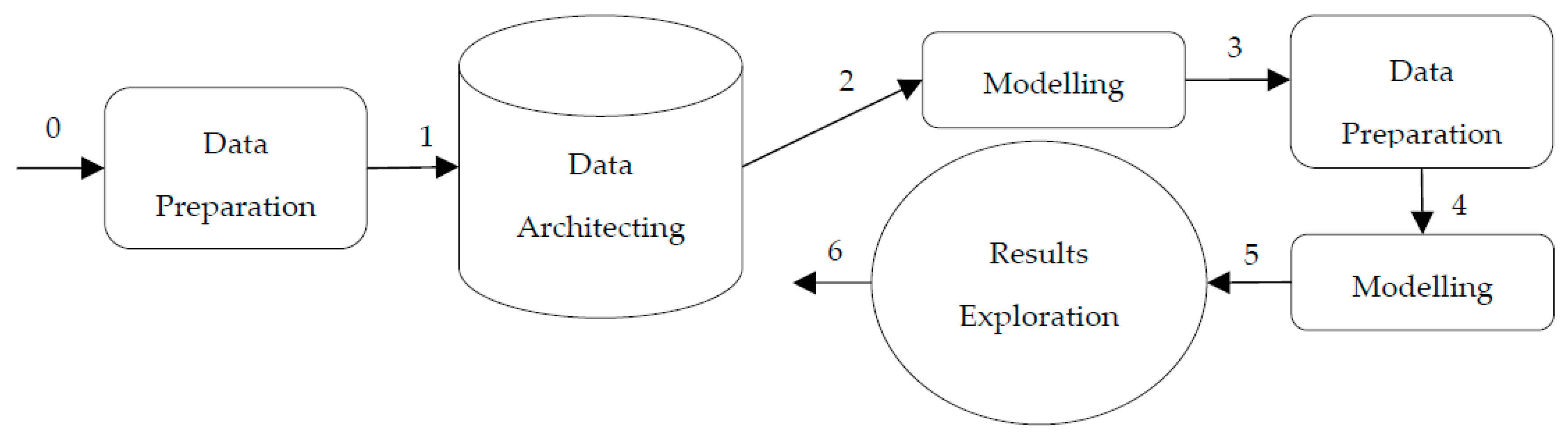
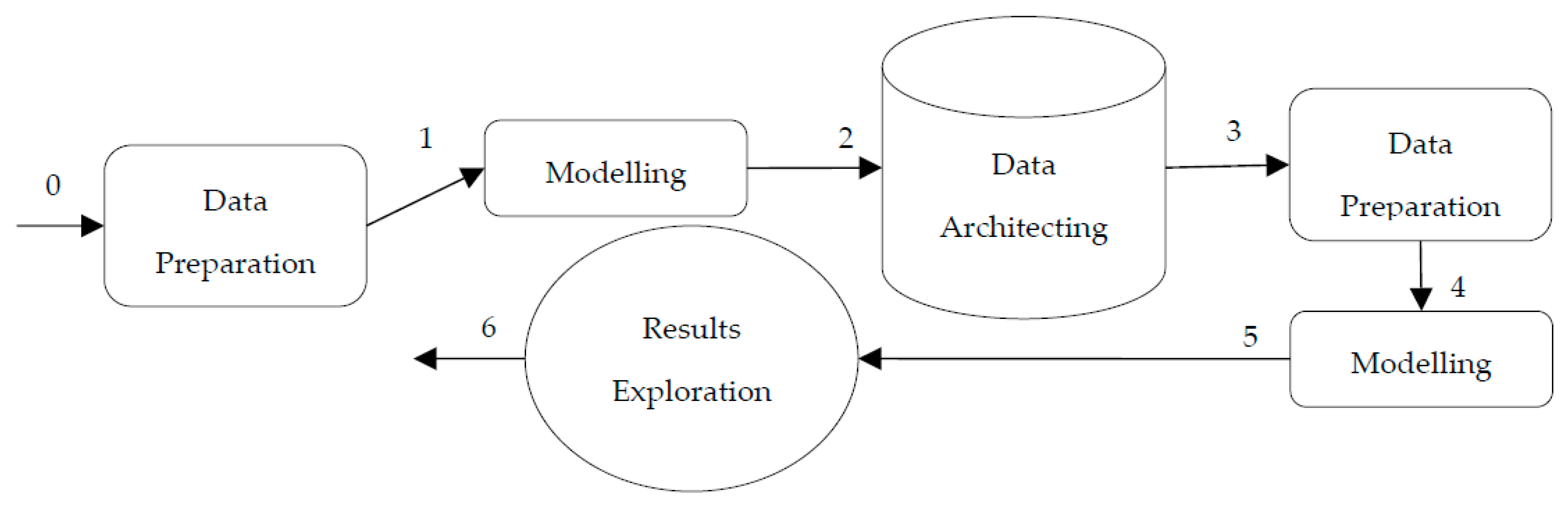
2. Data Science Trajectories Models of the Record Linkage Approaches

The DST model is an extension of the popular (de facto) CRISP-DM data mining and knowledge discovery project approach. The model was designed to make it more applicable to today’s data science projects, which typically include some kind of exploratory activities. The main components of the DST model then comprise the activities that come from the existing CRISP-DM approach, which are data management (denoted by the cylinder shape) and goal-driven activities (denoted by the rounded square shape). The DST model includes exploratory activities (denoted by the circle shape in the map) and the numbered arrows to show the transition between activities which start from 0. The list of all activities and some examples of DST can be referred to in [21].

2.1. The General Approach

The deterministic and probabilistic approach to record linkage can be seen as a four-step general approach in the DST map (see Figure 1) that consists of four activities including data preparation, data architecting, modelling, and results exploration. The data preparation activity is where data are processed, standardised and parsed [22] so that record pairs can be generated in the next activity of data architecting. Assuming that there are databases A and B, then there will be a total of A × B record pairs generated. The modelling activity is where the matching process takes place. This is when the field-wise comparison is conducted (similarity measure) and the composite weight (similarity score) for each record pair is determined. If blocking is considered, it will be within this activity. Lastly, the decision about linking is made when the results, or the composite weight vector, are explored in the last activity. The DST in Figure 1 was superimposed on the general record linkage processes [17] for better comparison.

2.2. The Two-Step Approach

The two-step record linkage approach (see Figure 2) also consists of the same activities as the general approach, with the addition of another data preparation activity in step 3 for the training data preparation; and a modelling activity in step 4 for record pair classification based on the trained classifier. Therefore, in total, there are six activities, and the first three are the same as the general approach. The two-step record linkage approaches usually conduct a binary classification; hence, the record pairs will be classified as linked or unlinked during the modelling activity. The performances are later evaluated in the exploration activity.

2.3. The Proposed Approach

The DST of the proposed method also consists of six steps, with the same elements as those in the DST for the two-step approach. The main difference between the approaches is in steps 1 and 2, where the modelling phase comes first in the proposed approach before data architecting (see Figure 3). In the proposed approach, step 1 represents the implementation of URF, where records from databases A and B will be combined to produce A + B records with the length of n and sent to the URF model. Step 2 represents the generation of record pairs from the upper triangle of the proximity matrix produced by URF. The total number of record pairs is then:

$$\frac{n\left(n-1\right)}{2}$$

(1)

The remaining steps then are the same as in the two-step approach, where training data are created in step 3 and used to train selected classifiers in step 4. The results are then evaluated in step 5, in the results exploration activity.

The two-step approach and the proposed approach differ not only in steps 1 and 2 of the DST map but also in the training data preparation in step 3. In Section 4.2.3, we propose three different constructions for selecting training data, and their details are discussed further.

3. Related Studies

We categorised training data preparation approaches based on the level of human involvement in labelling the instances for match and non-match sets. Full involvement was considered manual selection, minimal as semi-automatic, and non-involvement as automatic.

3.1. Manual Training Data Selection

Manually reviewing training data is an effective method for acquiring high-quality training data [23]. However, this procedure is expensive in terms of money or time. It is undeniable that humans are much better at identifying similarities compared to computer algorithms. Therefore, to produce high-quality training data, human power was employed in [12,24]. Similar human power employment was seen in [25,26] through crowdsourcing, but the main focus of these studies is producing smaller HITs (human intelligent tasks) that minimise the number of records that need to be manually compared. Since the process of determining the record pairs is still done by humans, we considered the crowdsourcing task a manual approach.

3.2. Semi-Automatic Training Data Selection

A small amount of human involvement in manual labelling can be seen in some active learning approaches, such as those in [23,27,28,29]. Active learning typically involves an iterative method in which humans are involved initially for some seed selection to train the classifier [23,28] or humans are involved in each loop for labelling pairs that are considered difficult to classify [27]. In the seed selection approach, the concern is to select pairs that are highly representative. The approach by [23] uses distinct record pairs sampled from each stratum based on field-wise comparison agreement. On the other hand [28], uses the entropy of the record pairs to establish those that are uncertain (with high entropy) and those that are of high confidence (low entropy). A much more recent active learning approach in entity resolution [29] formed training data by manual review, where record pairs under a certain limit (budget) were considered based on their informativeness measure. The selection of the record pairs was conducted iteratively by evaluating a selected similarity vector space where the entropy and uncertainty of the vector were considered. The approach was said to be independent of any classifiers and did not rely on the assumption that a higher similarity score leads to a matched record pair.

3.3. Automatic Training Data Selection

Automating the process of training data selection is still relevant for dealing with highly sensitive data [20]. In [20], an automatic seed selection was used, where the algorithm was based on the nearest-based approach proposed by [17,18]. The nearest-based approach uses a distance measure to select certain percentages of record pairs based on the distance of the similarity weight vectors from vectors containing only exact similarity and total dissimilarity. The weight vectors are then sorted according to their distance. The match pairs for the training data are selected from those closer to the high likelihood of matched pairs, and the non-match pairs are those closer to the high likelihood of non-matched pairs. In [17], the nearest-based selection was also considered for only choosing consecutively or only those with unique weight vectors. Balanced and imbalanced distributions were also evaluated. The results show that there is not much difference between unique and non-unique selection. However, the imbalanced training data size shows better results than a balanced size in most cases.

Along with the nearest-based approach, a threshold-based approach was also proposed by [17,18]. The threshold-based selection method selects record pairs whose similarity weight vectors are all within a certain distance from the set threshold. The nearest-based approach, however, generally outperformed the threshold-based approach [18]. The experiments in [17] also show that the results are highly sensitive to the threshold value. We believe that the threshold-based approach was not able to capture the proportion of the highly imbalanced class of the candidate record pairs. Since the nearest-based approach was able to explicitly set the percentage of records going to be considered in the match and non-match sets, an imbalanced proportion can be mirrored. As seen in [20], the match pairs were set to 0.01% and the non-match pairs were set to 1% for the automatic seed selection.

A recent study by [30] utilised the informativeness measure proposed by [29] and coupled it with the cosine similarity measure to select a certain number of high-quality record pairs with the highest score as the training dataset. Their experiments showed that such selection is better than random sampling from the whole record pair set or random sampling from the matched and non-matched record pair sets. Additionally, the authors of [31] proposed a novel data augmentation technique named EMix to generate training data, which was utilised in their MixER model. The experimental results demonstrated that the MixER model outperformed existing methods in recall and robustness.

4. Materials and Methods

4.1. Dataset

The first dataset used in this study can be found in the R RecordLinkage package, named RLdata500. It contains 500 records, with 50 duplicates. We only remove empty columns in the RLdata500, leaving the first name and last name fields, and expand the date of birth to three fields: day, month, and year.

The second dataset is the restaurant records collected from Zagat with 533 and Fodor with 331 observations of restaurant reviews that are now available from the R restaurant package. There are a total of 864 records with 112 duplicates. We cleaned the data by handling missing values and standardising the format, which included removing any additional information. We also expanded the phone number into three fields, where phn_1 consists of the first three digits, phn_2 contains the next three digits, and phn_3 contains the last four digits. The other fields included in the Restaurant dataset are name, address, city, and type.

We started off with these two datasets in this study since they contain fields of mixed data types (numbers and strings). Based on the initial study that we performed in [32], any number values were set as integer data types and strings as characters. Both datasets have a one-to-one relationship, which means that duplicate records have only one match.

4.2. Modelling, Data Architecting, and Data Preparation Activities

This section will discuss steps 2–3 of the DST map (see Figure 3) for the proposed approach, which involved modelling, data architecture, and data preparation activities. The remaining activities represent the second step of the two-step approach for classifying the record pairs. Although this paper’s main concern is on forming the training data, the only way to know the best construction was by looking at the classification results. Therefore, this study chooses RF [33] and support vector machine (SVM) [34]. The main reason for choosing these classifiers was because they both were able to handle data of mixed data types and were known to have been successfully applied for record pairs classification [17]. The R caret package was used at this stage since it offers a plethora of options for classifiers and allows easy switching between them. A cross-validation and confusion matrix is also available. The selected classifiers were then trained using five-fold cross-validation and repeated three times for parameter tuning. The confusion matrix was used to assess the classifiers’ performances based on the selected indexes.

4.2.1. The Modelling Activity

We proposed using URF as a similarity measure function, where a score is generated based on the normalised count of record pairs that fall on the same leaf in all the decision trees in the forest [33,35]. The URF will treat the linkage as a duplicate detection problem as all records will be combined and labelled as class 1. A generated record will be added and labelled as class 2. URF, then, will create decision trees based on the subsample of the two classes. The original data will then be compared in pairs on all trees to determine their proximity. The concept of proximity assumes that if the record pairs fall on the same leaf, then they are similar. The paper by [36] explains the algorithm of URF in detail.

Record pairs’ similarity score derived from the proximity matrix only considers elements where the row value is greater than the column. Formally, if we are to assume C as the proximity matrix with a cardinality of n × n, then C = ${\left(c_{ij}\right)}_{1 \le i, j \le n}$. To form the record pairs, only those elements where i < j were considered. The i value was the id for the first record, j for the second, and $c_{ij}$ was the pair similarity score. Since only half of the matrix was read, then the implementation of the record pair generation takes O(n²/2) times.

4.2.2. The Data Architecting Activity

Based on the ids of the record pairs, the ids were mapped back to the original records so that the Jaro–Winkler string comparator [37,38] can be applied for its corresponding string fields and absolute distance for numerical fields. These similarity measure functions were conducted to represent the pair’s fields as a single value and not as a field-wise comparison weight since the record pairs’ similarity score had already been calculated. The similarity score vector was also included so that the pairs could be sorted but later excluded from the training data as the training data will be labelled.

4.2.3. The Data Preparation Activity

The data preparation in step 3 was when the training data were constructed from the record pairs that were sorted in descending order based on the similarity score field. The training data follows three constructions that represent the selection of the labelled non-match record pairs, denoted as $p_{nm}$, that started at the bottom, the top, or are selected at random, after a lower threshold, denoted as $t_l$ (see Figure 4). The labelled match record pairs $p_m$ will always be from the top until the upper threshold $t_u$. The training data were then a mix of $p_m$ and $p_{nm}$. The remaining record pairs were the ones that were going to be the testing data or record pairs to be classified. However, record pairs with a similarity score of zero, denoted as $p_0$, were excluded as these pairs were assumed to be non-matches. For each of the constructions, a balanced (symmetry) and imbalanced (asymmetry) distribution will be tested. The imbalance distribution was decided based on a predetermined imbalance ratio. The algorithms that represent the complete training data construction for the bottom, top, and random constructions can be referred to as Algorithms 1, 2 and 3, respectively.

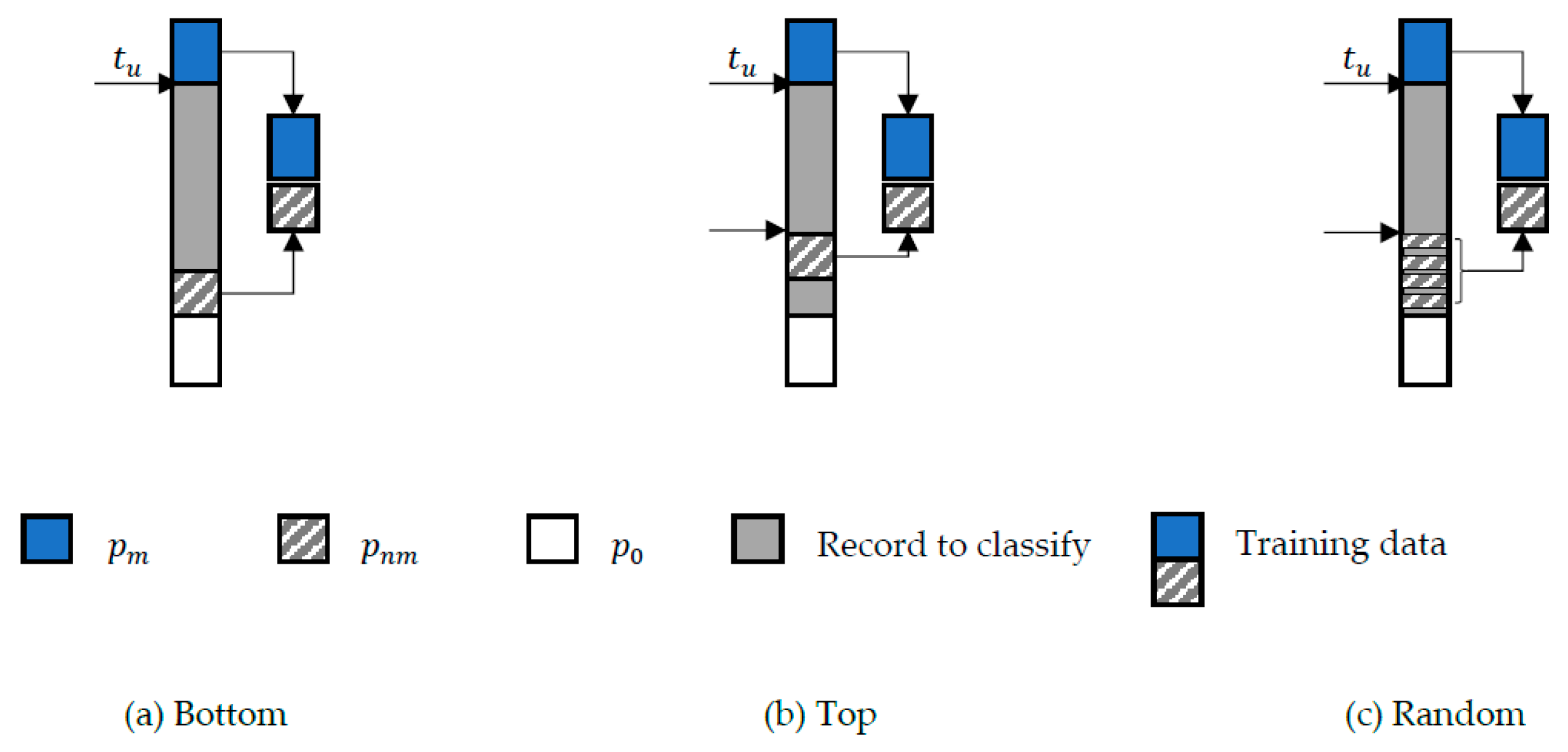
Algorithm 1. Bottom Selection.

Input:  – p, record pairs in descending order where similarity score > 0  – Set tu, r*//for balanced r* = 1 Output:  – tr—training data  – ts—record to classify Set pm ← p.similarity score ≥ tu Get pm length → l Set pnm ← last p with length (l × r*) Set pm.label ← “match” Set pnm.label ← “nonmatch” Set tr ← rbind(pm, pnm) Set ts ← p(−pm & −pnm) Remove similarity score column from tr and ts

Algorithm 2. Top Selection.

Input:  – p, record pairs in descending order where similarity score > 0  – Set tu, tl, r*//for balanced r* = 1 Output:  – tr—training data  – ts—record to classify Set pm ← p.similarity score ≥ tu Get pm length → l Set pnm ← from p where similarity score ≥ tl, with length (l × r*) Set pm.label ← “match” Set pnm.label ← “nonmatch” Set tr ← rbind(pm, pnm) Set ts ← p(−pm & −pnm) Remove similarity score column from tr and ts

Algorithm 3. Random Selection.

Input:  – p, record pairs in descending order where similarity score > 0  – Set tu, tl, r*//for balanced r* = 1 Output:  – tr—training data  – ts—record to classify Set pm ← p.similarity score ≥ tu Get pm length → l Set pnm ← randomly from p where similarity score ≥ tl, with length (l × r*) Set pm.label ← “match” Set pnm.label ← “nonmatch” Set tr ← rbind(pm, pnm) Set ts ← p(−pm & −pnm) Remove similarity score column from tr and ts

4.3. Classification Methods

Other than comparing RF and SVM based on all training data constructions, we also compared it with FSM, where the similarity measures were based on the expectation maximisation (EM) algorithm and EpiLink [39]. These methods are built into the RecordLinkage package as the emWeights and epiWeights functions [40]. The package also provides linkage using clustering methods. We used K-means [41] and bagged clustering (bclust) [42]. We categorise the clustering methods as unsupervised and include the URF within this category.

4.4. Classification Performance Measures and Training Data Quality

Due to the large number of true non-match (true negative) record pairs, the classification performances will be evaluated using performance indexes that exclude true negative (TN), such as precision, P = TP/TP + FP; recall, R = TP/TP + FN; and the F-measure, F₁ = 2(P × R)/(P + R). True positive (TP) is the number of correctly classified true matches, while false negative (FN) is the number of wrongly classified true matches (mismatches). The precision tells how well the classification process is doing in classifying the true matches, while the recall tells how well the classification process is doing in identifying all true matches. The F-measure is the harmonic mean between precision and recall and is used as the main index [43]. In the event of a tie in the F-measure, recall will be considered, as a higher recall indicates more true matches were discovered. Since this was an empirical study, no blocking was applied to the record pairs. The optimal threshold for the EM, EpiLink, and URF was decided based on the maximum F₁-score. Although these classification performance measures show how accurate the performance of classifiers is, we nevertheless used the measure to identify the best constructions of the training data.

The training data quality was decided based on the percentage of correctly labelled record pairs $p_m$ as matched and $p_{nm}$ as non-matched [17]. Determining the quality of the training data as well as the performances of all compared methods was made possible because the ground truth (gold standard) data were available for both datasets.

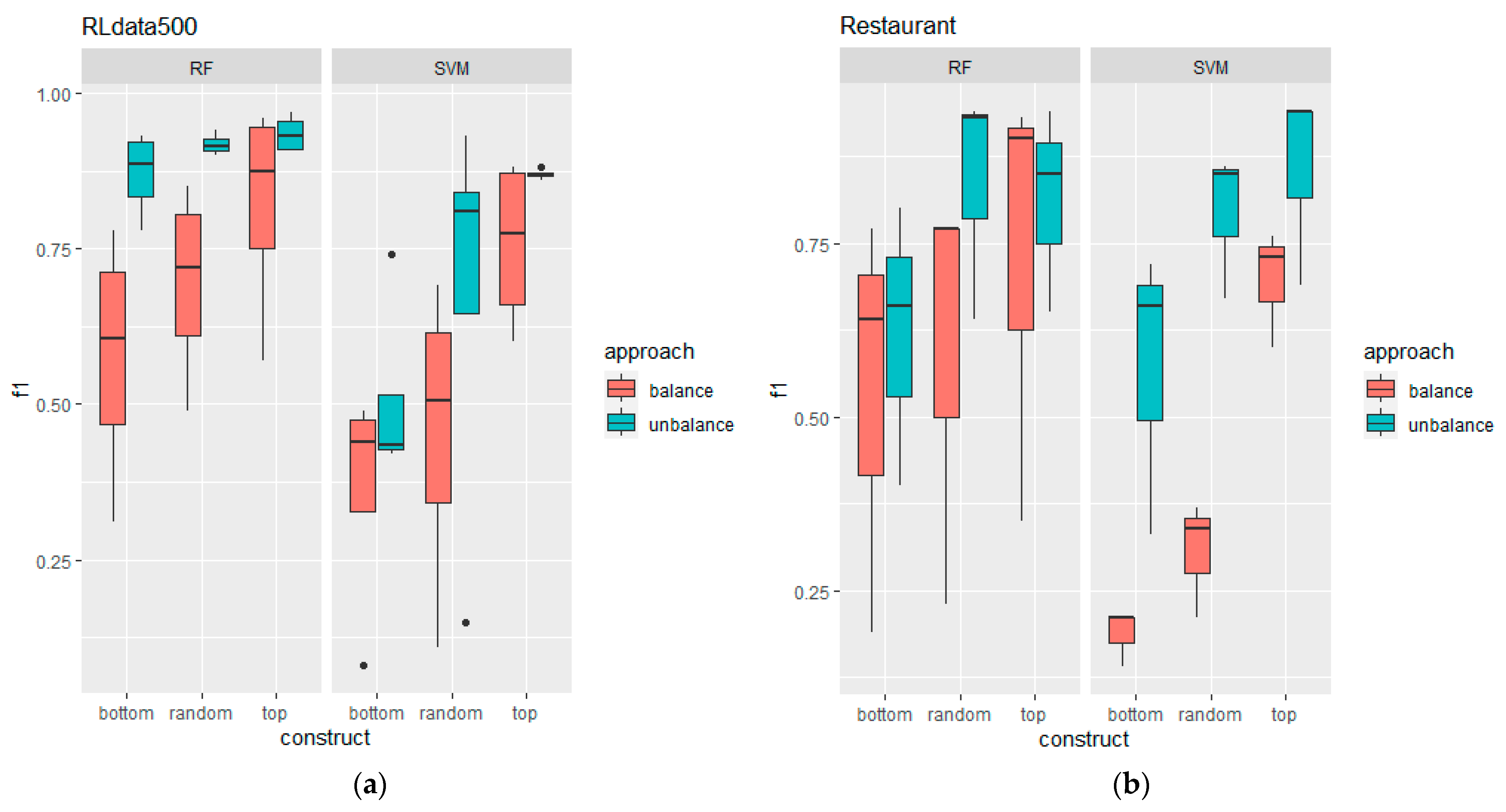
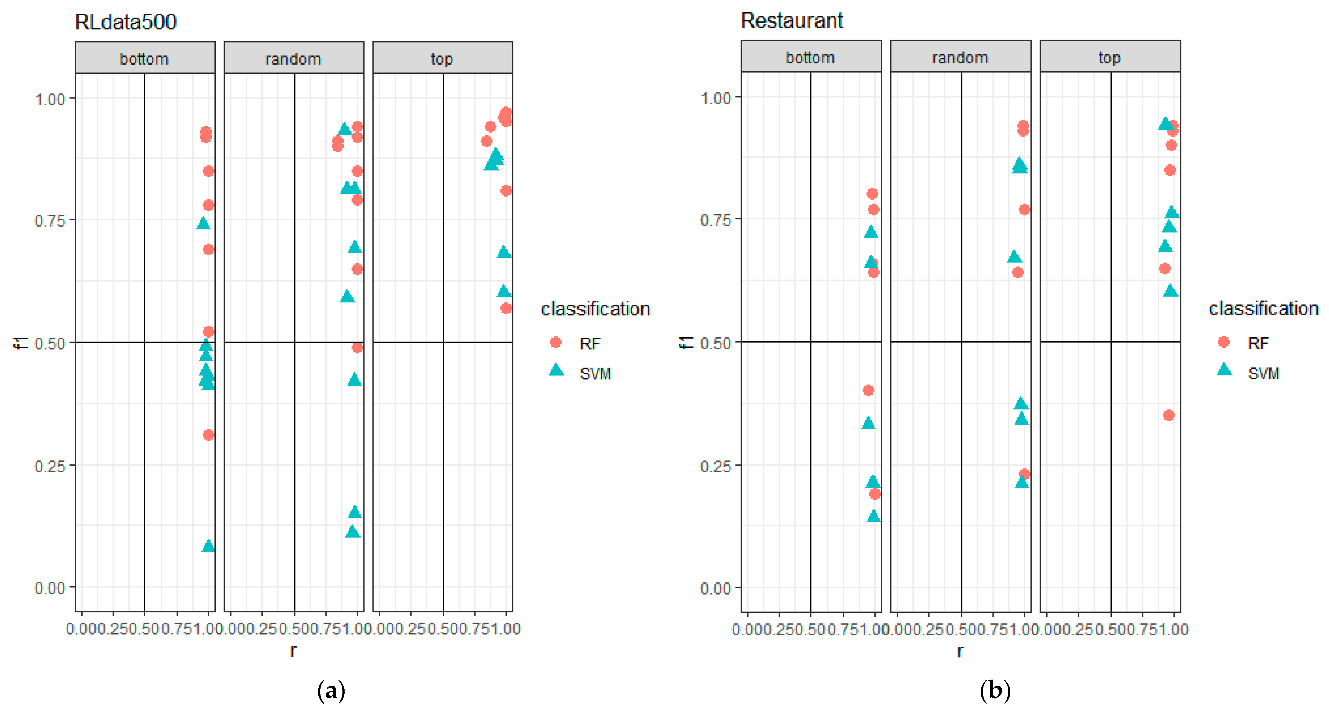
5. Results and Discussion

In total, the RLdata500 dataset produced 124,750 pairs, of which 74% were already considered non-matches since the similarity score was zero ($p_0$). As for the Restaurant dataset, there were 372,816 pairs, and $p_0$ was also 74%. When compared with the gold standard, the $p_0$ for both datasets were true non-match (quality was 100%). The nearest-based approach in [17,19] also excluded zero weighted scores in the training data.

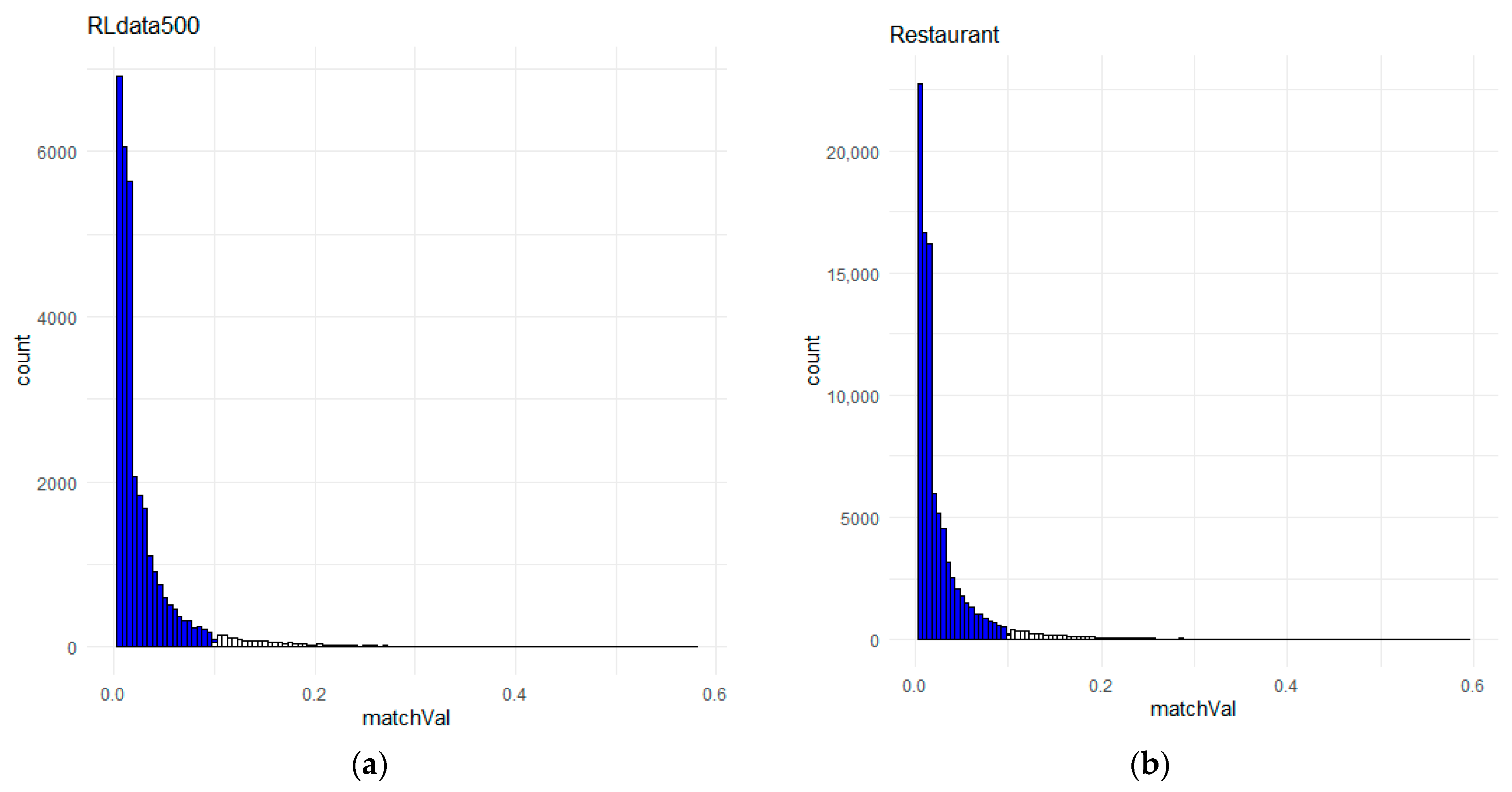
5.1. Setting Thresholds and Training Data Quality

Determining the $t_u$ in the training data creation is critical for distinguishing the matched record pairs. We had set $t_u$ to start at 0.9 and decreased the threshold by 0.1 at a time, and we observed the quality of the training data. The process was stopped once the match record pairs’ quality had worsened. The thresholds of 0.6 and 0.7 were the lowest $t_u$ for the Rldata500 and restaurant data, respectively (see

Table 1. Training data quality and the percentage of total training data over the record pairs excluding $p_0$.

Dataset		RLdata500								Restaurant
Upper Threshold		$${\mathit{t}}_{\mathit{u}} \ge \mathbf{0.9}$$		$${\mathit{t}}_{\mathit{u}} \ge \mathbf{0.8}$$		$${\mathit{t}}_{\mathit{u}} \ge \mathbf{0.7}$$		$${\mathit{t}}_{\mathit{u}} \ge \mathbf{0.6}$$		$${\mathit{t}}_{\mathit{u}} \ge \mathbf{0.9}$$		$${\mathit{t}}_{\mathit{u}} \ge \mathbf{0.8}$$		$${\mathit{t}}_{\mathit{u}} \ge \mathbf{0.7}$$
Imbalance Ratio		1:1	1:9	1:1	1:9	1:1	1:9	1:1	1:9	1:1	1:7	1:1	1:7	1:1	1:7
Training Set Quality	Match	100	100	100	100	100	100	97.62	97.62	100	100	100	100	92.42	92.42
	Bot, Non-match	100	100	100	100	100	100	100	100	100	100	100	100	100	100
	Top, Non-match	100	100	100	100	100	100	100	100	100	100	100	100	100	100
	Rand, Non-match	100	100	100	100	100	100	100	100	100	100	100	100	100	100
Training %		0.17	0.87	0.22	1.09	0.25	1.24	0.26	1.30	0.06	0.23	0.07	0.29	0.14	0.55

). As observed, the generated training data for all constructions produced training data of high quality, with the highest percentage of the training data over all records (excluding $p_0$) being just less than 1.5% for the RLdata500 and slightly over 0.5% for Restaurant datasets.

In setting the $t_l$, the challenge is to determine a value that will ensure only true non-matches are included. The lowest similarity score in the gold standard for RLdata500 was 0.11, so we set $t_l$ = 0.1. The same $t_l$ value was set for the Restaurant dataset for consistency even though there were three true matches with a similarity score below 0.1. Somehow, the true matches were not included in the non-match training data, and we believe this was because the distribution of the lower part of the similarity score vector was highly right-skewed (see Figure 5). However, this may have affected the performances of the classifiers, as the best F₁-score achieved was 0.94. The classifiers were able to distinguish two of the true matches (weights 0.03 and 0.09), but not one since its weight was 0.1.

5.2. Training Data Construction Performance

The initial setup for the training data only considers a balanced sample from the match ($p_m$) and non-match ($p_{nm}$) record pairs, as seen in [8]. This is because a classification model that is trained on a symmetric number of samples from each class or with a similar distribution of samples from each class helps to avoid bias towards one class and can lead to a more accurate and generalisable model. However, the results then showed both classifiers, RF and SVM, were not sufficient in discriminating the false matches (FP). Unlike [8], they have reported favourable results of using RF as compared to SVM (and other compared methods) when $p_{nm}$ was down-sampled to create the balanced classes. In general, down-sampling follows the random construction of selecting $p_{nm}.$ From our results (see Figure 6), the RF performance using balanced and random training data construction was also seen to be better than SVM for both datasets. However, the authors of [17] stated the need to reflect the highly imbalanced data in the training data and suggested the ratio r to be the number of true matches to the number of true false matches. The estimated r can then be derived by:

$$r=\frac{min\left(\left|A\right|,\left|B\right|\right)}{\left|W\right|-min\left(\left|A\right|,\left|B\right|\right)}$$

(2)

where W is the total number of weight vectors, which is the number of candidate record pairs after blocking.

In the study, the imbalanced training data were created by gradually increasing the ratio in $p_{nm}$ and it was found that a 1:9 imbalanced ratio of $p_m$ to $p_{nm}$ was ideal for the RLdata500 dataset and 1:7 for the Restaurant dataset. The imbalance ratio was found to follow the number of true matches to the number of distinctive records instead. As discovered by [23], training data do not need to follow the same proportion of all record pairs. Having training data that is able to capture all distinct record pairs is more important than having more samples in the training data, which has also been demonstrated by [30]. Following the notation in [17], the estimated imbalance ratio $r^{*}$ can be derived as follows:

$$r^{*}=\frac{min\left(\left|A\right|,\left|B\right|\right)}{\left|A\right|+\left|B\right|-min\left(\left|A\right|,\left|B\right|\right)}$$

(3)

The comparison of the F₁-score results between balanced and imbalanced training data is summarised in the boxplots shown in Figure 6. Upon initial examination, the imbalanced training data produced significantly better results collectively across all constructions for both datasets and classifiers. This suggests that intentionally choosing an asymmetrical training data distribution can help to counter the inherent imbalance in the record pairs distribution, forcing the classifiers to learn to handle bias. This is similar to [17], where their experiments showed that imbalanced training size was better than balanced in most cases. The plot also shows that the top and random constructions were always better than the bottom construction.

To determine which construction is better, a dot plot of the F₁-score against recall was used, and the plot area was divided into four quadrants. Since high F₁-score and recall values are preferable, the upper triangle of the top-right quadrant is the area of interest. Figure 7 shows the performances of the classifiers given the constructions, and it can be observed that the top construction places both classifiers in the top-right quadrant for the RLdata500 dataset. The Restaurant dataset also shows most instances of the top construction were in the top-right quadrant, except for one instance that was placed in the bottom-right, which indicated an F₁-score that was below 0.5, but the recall was greater than 0.5 (high in false matches). Despite that, as compared to the other two constructions, the top construction produced much better classification results for both classifiers for the given datasets.

When comparing the F₁-score of the proposed approach classifiers (RF, SVM) against the optimal threshold methods (EM, EpiLink) and the unsupervised approach (URF, K-means, and bclust) for the RLdata500 dataset using the top and imbalanced construction, the RF classifier achieved the highest score of 0.97 at $t_u=0.7$. The same construction produced the best F₁-score for the Restaurant dataset, with RF and SVM achieving the highest scores (0.94) at $t_u=0.9$ and $t_u=0.8$, respectively. However, the RF classifier had the highest recall value of 0.99 at $t_u=0.9$ and $t_u=0.8$ for the top and random construction. In our opinion, the top construction is preferred due to its simplicity, and promoting it for the Restaurant dataset would be consistent with the RLdata500 dataset. The previous best F₁-score and recall results were achieved by the optimal threshold approach using EM, with scores of 0.96 and 0.94 for the RLdata500 dataset, and by EpiLink with scores of 0.93 and 0.95 for the Restaurant dataset. On average, the top and imbalanced construction using RF classifier had improved the performances based on F₁-score by 1% and recall by 6.45%.

Table 2. Classification performance results for the proposed approach, the optimal threshold methods, and the unsupervised approach to record linkage.

Classification Approach	Dataset
	RLdata500			Restaurant
	Precision	Recall	F1-Score	Precision	Recall	F1-Score
EM	0.98	0.94	0.96	0.81	0.86	0.83
EpiLink	1	0.92	0.96	0.91	0.95	0.93
URF	1	0.82	0.9	0.85	0.65	0.73
K-Means	0.01	0.98	0.03	0	1	0
bclust	0.03	0.98	0.06	0.89	0.96	0.92
RF-T-tu ≥ 0.9	1	0.84	0.91	0.9	0.99	0.94
RF-T-tu ≥ 0.8	1	0.84	0.91	0.75	0.97	0.85
RF-T-tu ≥ 0.7	0.94	1	0.97	0.5	0.93	0.65
RF-T-tu ≥ 0.6	0.91	1	0.95
SVM-T-tu ≥ 0.9	0.84	0.92	0.88	0.94	0.94	0.94
SVM-T-tu ≥ 0.8	0.85	0.88	0.86	0.95	0.93	0.94
SVM-T-tu ≥ 0.7	0.82	0.92	0.87	0.55	0.93	0.69

shows the performance results of all the methods compared under the top and imbalanced constructions. The method with the highest performance index is in bold.

The best linkage results of using the proposed approach were then achieved by using the RF classifier under imbalanced data selected from the top construction. The best selection of training data for RLdata500 was at $t_u=0.7$ and $t_u=0.9$ for the Restaurant dataset. These two training data constructions only comprise 1.24% and 0.23% of the total records (excluding $p_0$), respectively, yet achieved comparable performance with the optimal threshold methods of EM and EpiLink.

Having training data that is of high quality definitely helps in the classification process for RF as well as SVM. Both of these classifiers were also known to work well in small training datasets [23], with the advantage of RF being that it is an assembly of decision trees that is able to minimise bias and variance [24]. Having RF as the best classifier in this study also supported one of the conclusions in [23], where tree-based classifiers work well in record linkage classification due to their low dimensionality ($p\ll n$) and simplicity of the underlying problem.

5.3. Study Limitations

Having access to the gold standard data enables us to identify the best construction for the training data. With knowledge of the similarity score in gold standard data, we were able to set optimal values for $t_u$ and $t_l$, and with knowledge of the number of matching records, we were able to set the optimal imbalance ratio. However, this kind of information is not typically available in real-world scenarios. Without the gold standard, determining the optimal values for $t_u$, $t_l$, and the imbalanced ratio can be challenging. Therefore, the current state of training data preparation in this study is still considered semi-automatic, as it requires human inspection and intervention to set these parameters.

It is also important to note that this study is limited to datasets containing only strings and numeric datatypes. The success of a linkage process depends heavily on the quality of the data and the available fields [4]. While we used two public datasets in our study, the different treatments applied to the fields make it difficult to compare our results with those of other studies. As a result, we only compared our method with the ones stated in this study, and our main focus was not to determine the best classifier but to identify the best construction method for the training data.

6. Conclusions

In conclusion, this study presented a novel approach to record linkage that is based on a two-step process utilising URF as a similarity measure in the first step. The URF model simplifies the similarity measure process by using decision trees to handle pairwise comparisons. The proximity values produced by the decision trees in the forest were used as the similarity score between record pairs, which facilitated the creation of high-quality training data. The study tested three different constructions for the training data on two datasets (RLdata500 and Restaurant) with two classifiers, RF and SVM. Different distributions of the training data were also evaluated. The results showed that the imbalanced (asymmetrical) distribution with non-matched record pairs chosen from the top construction consistently produced the best performance when using the RF classifier, which outperformed all other linkage methods tested, including FSM methods using epi- and em-weights, and the unsupervised K-means, bclust, and URF methods. While more work is needed to automate the determination of optimal thresholds and imbalance ratios for this approach, this study highlights its potential for improving the record linkage process. Future research will test the proposed approach on different datasets to confirm the best training data constructions and classifiers. Overall, this study demonstrates the effectiveness of the proposed approach, which on average improved the F₁-score by 1% and recall by 6.45% compared to the previous best results achieved by the EM and EpiLink methods.

References

1. Talburt, J.R. (Ed.) Entity Resolution and Information Quality; Morgan Kaufman: Burlington, MA, USA, 2011; ISBN 9780123819727. [Google Scholar]
2. Dunn, H.L. Record Linkage. Am. J. Public Health Nations Health 1946, 36, 1412–1416. [Google Scholar] [CrossRef] [PubMed]
3. Winkler, W.E. Methods for Evaluating and Creating Data Quality. Inf. Syst. 2004, 29, 531–550. [Google Scholar] [CrossRef]
4. Zhu, Y.; Matsuyama, Y.; Ohashi, Y.; Setoguchi, S. When to Conduct Probabilistic Linkage vs. Deterministic Linkage? A Simulation Study. J. Biomed. Inform. 2015, 56, 80–86. [Google Scholar] [CrossRef] [PubMed]
5. Herzog, T.N.; Scheuren, F.J.; Winkler, W.E. Data Quality and Record Linkage Techniques; Springer: New York, NY, USA, 2007; ISBN 9780387695020. [Google Scholar]
6. Fellegi, I.P.; Sunter, A.B. A Theory for Record Linkage. J. Am. Stat. Assoc. 1969, 64, 1183–1210. [Google Scholar] [CrossRef]
7. Christen, P. Data Matching: Concepts and Techniques for Record Linkage, Entity Resolution, and Duplicate Detection; Springer: Berlin/Heidelberg, Germany, 2012; ISBN 3642311636. [Google Scholar]
8. Mason, L.G. A Comparison of Record Linkage Techniques; Quarterly Census of Wages and Employment (QCEW): Washington, DC, USA, 2018; pp. 2438–2447. [Google Scholar]
9. Gu, L.; Baxter, R. Decision Models for Record Linkage. In Data Mining; Springer: Berlin/Heidelberg, Germany, 2006; Volume 3755, pp. 146–160. [Google Scholar] [CrossRef]
10. Elfeky, M.G.; Verykios, V.S.; Elmagarmid, A.K. TAILOR: A Record Linkage Toolbox. In Proceedings of the 18th International Conference on Data Engineering, San Jose, CA, USA, 28 February–1 March 2002; pp. 17–28. [Google Scholar]
11. Goiser, K.; Christen, P. Towards Automated Record Linkage. Conf. Res. Pract. Inf. Technol. Ser. 2006, 61, 23–31. [Google Scholar]
12. Jiao, Y.; Lesueur, F.; Azencott, C.A.; Laurent, M.; Mebirouk, N.; Laborde, L.; Beauvallet, J.; Dondon, M.G.; Eon-Marchais, S.; Laugé, A.; et al. A New Hybrid Record Linkage Process to Make Epidemiological Databases Interoperable: Application to the GEMO and GENEPSO Studies Involving BRCA1 and BRCA2 Mutation Carriers. BMC Med. Res. Methodol. 2021, 21, 155. [Google Scholar] [CrossRef] [PubMed]
13. Ebeid, I.A.; Talburt, J.R.; Hagan, N.K.A.; Siddique, M.A.S. ModER: Graph-Based Unsupervised Entity Resolution Using Composite Modularity Optimization and Locality Sensitive Hashing. Int. J. Adv. Comput. Sci. Appl. 2022, 13, 1–18. [Google Scholar] [CrossRef]
14. Yao, D.; Gu, Y.; Cong, G.; Jin, H.; Lv, X. Entity Resolution with Hierarchical Graph Attention Networks. In Proceedings of the 2022 International Conference on Management of Data, Philadelphia, PA, USA, 12–17 June 2022; ACM: New York, NY, USA, 2022; pp. 429–442. [Google Scholar]
15. Kirielle, N.; Christen, P.; Ranbaduge, T. Unsupervised Graph-Based Entity Resolution for Complex Entities. ACM Trans. Knowl. Discov. Data 2023, 17, 12. [Google Scholar] [CrossRef]
16. Abassi, M.E.; Amnai, M.; Choukri, A.; Fakhri, Y.; Gherabi, N. Matching Data Detection for the Integration System. Int. J. Electr. Comput. Eng. 2023, 13, 1008–1014. [Google Scholar] [CrossRef]
17. Christen, P. A Two-Step Classification Approach to Unsupervised Record Linkage. Conf. Res. Pract. Inf. Technol. Ser. 2007, 70, 111–119. [Google Scholar]
18. Christen, P. Automatic Record Linkage Using Seeded Nearest Neighbour and Support Vector Machine Classification. In Proceedings of the 14th ACM SIGKDD International Conference on Knowledge Discovery and Data Mining, Las Vegas, NV, USA, 24 August 2008; ACM: New York, NY, USA, 2008; pp. 151–159. [Google Scholar]
19. Christen, P. Automatic Training Example Selection for Scalable Unsupervised Record Linkage. In Proceedings of the Advances in Knowledge Discovery and Data Mining: 12th Pacific-Asia Conference, Osaka, Japan, 20–23 May 2008; Volume 5012, pp. 511–518. [Google Scholar] [CrossRef]
20. Jurek, A.; Hong, J.; Chi, Y.; Liu, W. A Novel Ensemble Learning Approach to Unsupervised Record Linkage. Inf. Syst. 2017, 71, 40–54. [Google Scholar] [CrossRef]
21. Martinez-Plumed, F.; Contreras-Ochando, L.; Ferri, C.; Hernandez-Orallo, J.; Kull, M.; Lachiche, N.; Ramirez-Quintana, M.J.; Flach, P. CRISP-DM Twenty Years Later: From Data Mining Processes to Data Science Trajectories. IEEE Trans. Knowl. Data Eng. 2021, 33, 3048–3061. [Google Scholar] [CrossRef]
22. Winkler, W.E. Matching and Record Linkage. Wiley Interdiscip. Rev. Comput. Stat. 2014, 6, 313–325. [Google Scholar] [CrossRef]
23. Sariyar, M.; Borg, A. Bagging, Bumping, Multiview, and Active Learning for Record Linkage with Empirical Results on Patient Identity Data. Comput. Methods Programs Biomed. 2012, 108, 1160–1169. [Google Scholar] [CrossRef] [PubMed]
24. Treeratpituk, P.; Giles, C.L. Disambiguating Authors in Academic Publications Using Random Forests Categories and Subject Descriptors. In Proceedings of the 9th ACM/IEEE-CS Joint Conference on Digital Libraries, Austin, TX, USA, 15–19 June 2009; pp. 39–48. [Google Scholar]
25. Wang, J.; Kraska, T.; Franklin, M.J.; Feng, J. CrowdER: Crowdsourcing Entity Resolution. Proc. VLDB Endow. 2012, 5, 1483–1494. [Google Scholar] [CrossRef]
26. Gottapu, R.D.; Dagli, C.; Ali, B. Entity Resolution Using Convolutional Neural Network. Procedia Comput. Sci. 2016, 95, 153–158. [Google Scholar] [CrossRef]
27. Sarawagi, S.; Bhamidipaty, A. Interactive Deduplication Using Active Learning. In Proceedings of the Eighth ACM SIGKDD International Conference on Knowledge Discovery and Data Mining, Edmonton, AB, Canada, 23–26 June 2002; pp. 269–278. [Google Scholar] [CrossRef]
28. Kasai, J.; Qian, K.; Gurajada, S.; Li, Y.; Popa, L. Low-Resource Deep Entity Resolution with Transfer and Active Learning. In Proceedings of the 57th Annual Meeting of the Association for Computational Linguistics, Florence, Italy, 28 July–2 August 2019; pp. 5851–5861. [Google Scholar] [CrossRef]
29. Christen, V.; Christen, P.; Rahm, E. Informativeness-Based Active Learning for Entity Resolution. In Proceedings of the European Conference on Principles of Data Mining and Knowledge Discovery, Ghent, Belgium, 14–18 September 2020; Springer: Berlin/Heidelberg, Germany, 2020; pp. 125–141. [Google Scholar]
30. Laskowski, L.; Sold, F. Explainable Data Matching: Selecting Representative Pairs with Active Learning Pair-Selection Strategies. In Lecture Notes in Informatics (LNI), Proceedings—Series of the Gesellschaft fur Informatik (GI); König-Ries, B., Scherzinger, S., Lehner, W., Vossen, G., Eds.; Gesellschaft für Informatik e.V.: Dresden, Germany, 2023; Volume P-331, pp. 1099–1104. [Google Scholar]
31. Wu, H.; Li, S. MixER: Linear Interpolation of Latent Space for Entity Resolution. Complex Intell. Syst. 2023, 1–20. [Google Scholar] [CrossRef]
32. Omar, Z.A.; Abu Bakar, M.A.; Zamzuri, Z.H.; Ariff, N.M. Duplicate Detection Using Unsupervised Random Forests: A Preliminary Analysis. In Proceedings of the 2022 3rd International Conference on Artificial Intelligence and Data Sciences (AiDAS), Ipoh, Malaysia, 7–8 September 2022; pp. 66–71. [Google Scholar]
33. Breiman, L. Random Forests. Mach. Learn. 2001, 45, 5–32. [Google Scholar] [CrossRef]
34. Cortes, C.; Vapnik, V. Support-Vector Networks. Mach. Learn. 1995, 20, 273–297. [Google Scholar] [CrossRef]
35. Cutler, A.; Cutler, D.R.; Stevens, J.R. Random Forests. In Ensemble Machine Learning; Zhang, C., Ma, Y., Eds.; Springer: New York, NY, USA, 2012; ISBN 978-1-4419-9325-0. [Google Scholar]
36. Afanador, N.L.; Smolinska, A.; Tran, T.N.; Blanchet, L. Unsupervised Random Forest: A Tutorial with Case Studies. J. Chemom. 2016, 30, 232–241. [Google Scholar] [CrossRef]
37. Jaro, M.A. Advances in Record-Linkage Methodology as Applied to Matching the 1985 Census of Tampa, Florida. J. Am. Stat. Assoc. 1989, 84, 414–420. [Google Scholar] [CrossRef]
38. Winkler, W.E. String Comparator Metrics and Enhanced Decision Rules in the Fellegi-Sunter Model of Record Linkage. In Proceedings of the Annual Meeting of the American Statistical Association, Anaheim, CA, USA, 6–9 August 1990; pp. 354–359. [Google Scholar]
39. Contiero, P.; Tittarelli, A.; Tagliabue, G.; Maghini, A.; Fabiano, S.; Crosignani, P.; Tessandori, R. The EpiLink Record Linkage Software: Presentation and Results of Linkage Test on Cancer Registry Files. Methods Inf. Med. 2005, 44, 66–71. [Google Scholar] [CrossRef] [PubMed]
40. Sariyar, M.; Borg, A. The Recordlinkage Package: Detecting Errors in Data. R J. 2010, 2, 61–67. [Google Scholar] [CrossRef]
41. Macqueen, J. Some Methods for Classification and Analysis of Multivariate Observation. In Proceedings of the 5th Berkeley Symposium on Mathematical Statistics and Probability, Berkeley, CA, USA, 21 June–18 July 1965; Volume 1, pp. 281–297. [Google Scholar]
42. Leisch, F. Bagged Clustering. Adapt. Inf. Syst. Model. Econ. Manag. Sci. 1999, 51, 11. [Google Scholar]
43. Christen, P.; Goiser, K. Quality and Complexity Measures for Data Linkage and Deduplication. Stud. Comput. Intell. 2007, 43, 127–151. [Google Scholar] [CrossRef]
Figure 1. DST map of deterministic and probabilistic record linkage approaches imposed on the general record linkage process.
Symmetry 15 01060 g001
Figure 2. DST map of the two-step record linkage approach.
Symmetry 15 01060 g002
Figure 3. DST map of the proposed approach.
Symmetry 15 01060 g003
Figure 4. Proposed method training data constructions where (a) the non-match training data were taken from the bottom, (b) the non-match training data were taken after the specified lower threshold, and (c) the non-match training data were taken at random after the specified lower threshold.
Symmetry 15 01060 g004
Figure 5. The lower half of the similarity weight vector distribution, where the blue bars indicate the candidate record pairs for non-match training data, where (a) is the distribution for RLdata500 and (b) is the distribution for the Restaurant dataset.
Symmetry 15 01060 g005
Figure 6. Boxplot comparison between balanced and imbalanced training data for both classifiers, RF and SVM, where comparison (a) is on the RLdata500 dataset and comparison (b) is on the Restaurant dataset.
Symmetry 15 01060 g006
Figure 7. Dot plot comparison for the three constructions, where the comparisons were based on F1-score against recall for (a) the RLdata500 dataset and (b) the Restaurant dataset.
Symmetry 15 01060 g007