A Multigoal Path-Planning Approach for Explosive Ordnance Disposal Robots Based on Bidirectional Dynamic Weighted-A* and Learn Memory-Swap Sequence PSO Algorithm

Abstract

In order to protect people’s lives and property, increasing numbers of explosive disposal robots have been developed. It is necessary for an explosive ordinance disposal (EOD) robot to quickly detect all explosives, especially when the location of the explosives is unknown. To achieve this goal, we propose a bidirectional dynamic weighted-A star (BD-A*) algorithm and a learn memory-swap sequence particle swarm optimization (LM-SSPSO) algorithm. Firstly, in the BD-A* algorithm, our aim is to obtain the shortest distance path between any two goal positions, considering computation time optimization. We optimize the computation time by introducing a bidirectional search and a dynamic OpenList cost weight strategy. Secondly, the search-adjacent nodes are extended to obtain a shorter path. Thirdly, by using the LM-SSPSO algorithm, we aim to plan the shortest distance path that traverses all goal positions. The problem is similar to the symmetric traveling salesman problem (TSP). We introduce the swap sequence strategy into the traditional PSO and optimize the whole PSO process by imitating human learning and memory behaviors. Fourthly, to verify the performance of the proposed algorithm, we begin by comparing the improved A* with traditional A* over different resolutions, weight coefficients, and nodes. The hybrid PSO algorithm is also compared with other intelligent algorithms. Finally, different environment maps are also discussed to further verify the performance of the algorithm. The simulation results demonstrate that our improved A* algorithm has superior performance by finding the shortest distance with less computational time. In the simulation results for LM-SSPSO, the convergence rate significantly improves, and the improved algorithm is more likely to obtain the optimal path.

1. Introduction

Global terrorist activities are on the rise, and it is easy for extremist actions to proliferate. Terrorism is a serious threat to the civilized world. To quickly and efficiently deal with explosives, various EOD equipment has been developed, such as the Andros series EOD robot [1], RMI-9WT [2], Packbot-EOD [3], etc. EOD robots can replace people in carrying out extremely hazardous tasks such as detecting, inspecting, grabbing, and transporting suspicious explosives in a dangerous environment. Many countries have developed different kinds of EOD robots. For example, the British Morfax corporation has invented an EOD robot called Wheelbarrow [4]. It is one of the most famous EOD robots in the world, possessing good vehicle mobility and explosive disposal performance. Meanwhile, American Remotec has developed an EOD robot called Andros F6A [5], which is used to help the police complete security tasks. It consists of a mobile carrier and a manipulator. The carrier is an articulated walking chassis that helps the robot adapt to complex terrain such as sloping, sandy, or rugged surfaces. The Chinese Shenyang Institute of Automation has invented the Lingxi-B EOD robot [6], which has three cameras; EOD personnel can accurately control the robot over long distances with cabled or cableless operations.

The path planning problem has attracted many researchers’ attention, and it is currently one of the biggest hotspots in the EOD robot control area. The main goal of path planning is to construct a collision-free path that allows the robot to move from the start position to the goal position in a given environment. Over the past few decades, a considerable amount of path planning algorithms have been proposed, such as artificial potential fields (APF) [7], genetic algorithm (GA) [8,9], harmony search algorithm (HSA) [10], A* algorithm [10,11,12], particle swarm optimization (PSO) [13,14], ant colony optimization (ACA) [15], rapidly exploring random tree. (RRT) [16,17], neural networks [18], etc. Pak et al. [19] proposed a path planning algorithm for smart farms by using simultaneous localization and mapping (SLAM) technology. In the study, A*, D*, RRT, and RRT* are compared to solve a short-distance path planning problem with static obstacles, longest-distance path planning problem with static obstacles, and a path planning problem with dynamic obstacles. The results showed that the A* algorithm is suitable when solving the path planning problem. Zeyu Tian et al. [20] introduce a SLAM construction based on the RRT algorithm to solve the path planning problemm which is considered as a partially observable Markov decision process (POMDP). The boundary points are extracted, and the global RRT tree are introduced with adaptive step. The results show that when solving the problem of local RRT boundary detection, the tree is reset to accelerate the detection of the boundary points around the robot and when solving the problem of the global RRT boundary detection process, the generated RRT tree can also continue to grow, so that the small corners and the robot’s boundary points can also be detected in the end. An RRT-based path planning method for two-dimensional building environments was proposed by Yiqun Dong et al. [21]. To minimize the planning time, the idea of biasing the RRT tree growth in more focused ways was used, the results show that the proposed RRT algorithm is faster than the other baseline planners such as RRT, RRT*, A*-RRT, Theta*-RRT, and MARRT. Symmetry is widely used in path planning. A* is a popular algorithm based on graph search. The method searches from the current node to surrounding nodes; this search process is symmetrical. The A* algorithm [22,23] is one of the best-known heuristic path planning algorithms. It was proposed by Peter Hart et al. in 1968. It is widely used due to its simple principle, high efficiency, and modifiability. It evaluates the path by estimating the cost value of the current node’s extensible nodes in the search area and guides the search toward the goal by selecting the lowest cost from the current node’s adjacent nodes. Although the traditional A* algorithm shows good performance, it may fall into a failed search state, and its speed is slow. Consequently, many scholars have proposed improved algorithms. Ruijun Yang and Liang Cheng [24] proposed an improved A* algorithm with an updated weights, which considers the degree of channel congestion in a restaurant using a gray-level model. The results show that the service robot can effectively avoid crowded channels in the restaurant and complete various tasks in a restaurant environment. Anh Vu Le et al. [25] invented a modified A* algorithm for efficient coverage path planning. They introduced zigzag thought into the traditional A* algorithm. The results show that the modified A* algorithm can generate waypoints to cover narrow spaces as well as efficiently maximize the coverage area. Erke Shang et al. [26] proposed a novel A* algorithm that considers evaluation standards, guidelines, and key points. The improved A* algorithm uses a new evaluation standard to measure the performance of many algorithms and selects appropriate parameters for the proposed A* algorithm. The experimental results demonstrated that the algorithm is robust and stable. Gang Tang et al. [27] proposed an improved geometric A* algorithm by introducing the filter function and the cubic B-spline curve. The improved strategy can reduce redundant nodes and effectively counter the problems associated with long distances.

Inspired by nature, PSO [28] is first introduced by Kennedy and Eberhart in 1995. This biological heuristic algorithm is widely used in path planning [29], complex optimization problems [30], inverse kinematics solutions [31], etc. In particular, the application of PSO in path planning has attracted the attention of many scholars. An improved PSO algorithm is proposed by Yong Zhang et al. [32] to determine the shortest and safest path problem. In their paper, the path plan problem is described as a constrained multiobjective problem. A membership function that considers both the degree of risk and the distance of the path is proposed to resolve the issue. The results showed that the improved algorithm can generate high-quality Pareto optimal paths to solve the robot planning path in an uncertain dangerous environment. Mihir Kanta Rath and B.B.V.L. Deepak [33] established a PSO-based system architecture to solve the robot path planning problem in a dynamic environment. The main goal of the proposed algorithm is to find the shortest possible path with obstacle avoidance. The simulation showed that the objective function successfully improves the efficiency of path planning in various environments.

Before the EOD robot removes explosives, searching for and finding the explosives from all the suspicious positions where terrorists may have hidden them is vital. Most studies only considered the planning of the path from one initial position to one goal position. Some additional problems that also need to be solved, however, are that the terrorists may hide multiple explosives in different positions. Furthermore, as the number of goal positions increases, the time needed to compute the path increases. It is particularly important to remove explosives quickly, as they may detonate at any time. The proposed algorithms are always time-consuming and easily fall into the local optimum. Thus, the EOD robot needs to plan the shortest path to detect multiple suspicious positions as quickly as possible. In this study, we focuse on the shortest distance path of traversing multiple goal positions while considering computation time optimization. The contributions of this study are as follows:

(1) A bidirectional dynamic weighted A* algorithm is proposed to reduce the calculation time. By using the grid method, the environment map is established to introduce the obstacle, initial position, and goal position information. The path planning problem is divided into two subproblems: one is the shortest path between any two positions, and the other is the shortest path for traversing all goal positions. Firstly, to ensure the problem is clearly described, the mathematical model is also presented. Then, we optimize the computation time by improving the A* algorithm with a novel dynamic OpenList cost weight strategy and a bidirectional search strategy. Finally, the adjacent nodes are expanded to 16 to obtain the shortest distance between any two positions. The simulation results of the improved strategies are analyzed and discussed.

(2) A learn-memory strategy is introduced to the PSO algorithm to enhance the exploration ability. The LM strategy imitates the behaviors of human learning and memory, such as comparison, analysis, association, retention, forgetting–reinforcement, and divergent thinking, to optimize the initial solutions, maintain the diversity of the swarm, improve the quality of solutions, etc. In the proposed algorithm, we obtain new particles by optimizing the nodes in one particle or between particles, learning some features or figures that exist to generate new excellent particles, etc.

(3) A swap-sequence strategy is introduced to the PSO algorithm to maintain the diversity of the swarm. The swap sequence strategy is introduced into the process of forgetting–reinforcement. By using the strategy, the traditional could make PSO avoid falling into local optimum. The performance of the LM-SSPSO algorithm is also compared with that of ACO, Tabu search (TB), swap sequence particle swarm optimization (SSPSO), and several other intelligent algorithms.

(4) The performance of the proposed algorithm is verified. To confirm the effectiveness of the proposed algorithm, different environment maps are also designed and analyzed. Finally, the conclusions of this paper are given.

The remainder of this paper is organized as follows: In Section 2, the environment map construction for path planning is established, and the mathematical model is presented. Then, in Section 3, an improved A* algorithm for the shortest distance path between any two goal positions and the computation time optimization are described and detailed. In Section 4, an LM-SSPSO algorithm is proposed for optimizing the path of traversing all goal positions. In Section 5, the experiments are designed and compared to further verify the effectiveness of the proposed approach. Finally, the conclusion and perspectives are given in Section 6.

2. Environment Representation and Mathematical Model

In this study, our goal was to improve the efficiency of path planning. The EOD robot path planning problem can be stated as follows: considering a cluttered environment that consists of an initial position and multiple suspicious positions, it is necessary to plan a collision-free path for the EOD robot moving from the initial position to multiple suspicious positions so that the robot can find all the hidden explosives. We plan the optimal path by considering the following two aspects. One is to obtain the shortest distance path between any two positions (including the initial position and the goal positions), and the other is to plan the shortest path where the EOD robot traverses all goal positions and returns to the initial position.

2.1. Grid-Based Environment Modeling and Definitions

For the path planning investigated in this paper, the environmental model is crucial. To describe environmental information, many methods have been developed. These include the grid method [34], visibility graph [35], Voronoi diagram [36], etc. The grid method is first proposed by W.E. Howden in 1968. It is one of the most widely used environment modeling methods that records the obstacle and path information. The main idea of the method is to divide the environment map into many small grids and to describe the free space and obstacle space efficiently. In this paper, we use the grid-based map to record the EOD robot environment information.

When the EOD robot moves around suspicious positions, the planned path should enable the robot to quickly and efficiently locate explosives. However, it is not easy to satisfy both of the following goals: one is that the final path should enable the robot to search around the suspicious position, so that the explosives can be detected effectively; the other is that the path should be as short as possible and that the robot needs to know where to stop before detecting explosives and where to go after detecting one in a suspicious position. To simplify the search process and to facilitate the detection of explosives, we define the EOD robot as a mass point and manually select three goal positions around each suspicious position, instead of moving all around it to detect explosives. As shown in Figure 1, the grid map is $180\times 180$. The contour area that the EOD robot cannot pass is marked with a black square; the area where the EOD can pass is marked with a white square that represents a free grid. The grid is marked with a red square that represents the initial position. The obstacle areas named {A, B, C, D, E} in the environment map are the suspicious positions. Each suspicious position is surrounded by three goal grids, which represent goal positions and are marked in fuchsia. There are 15 goal positions in total. All of the positions are named {2, 3, 4…15, 16}. The goal of the path planning is to plan an obstacle avoidance path for the EOD robot moving from the initial position, going through all of the 15 goal positions, and returning to the initial position at the end. To plan the path effectively, we establish a planar rectangular coordinate XOY and use the serial number method to encode the grids. In the XOY coordinates, the bottom left of the map is the origin; we encode the grid from bottom to top and left to right. The relationship between the grid number and grid coordinate is as follows:

$$\left\{\begin{array}{c}Nco{r}_i=(x_i-1)n+y_i\\ x_i=\frac{Nco{r}_i-y_i}{n}+1\\ y_i=Nco{r}_i-(x_i-1)n\end{array}\right.$$

(1)

where $Nco{r}_i$ represents the grid number, $(x_i,y_i)$ represents the grid coordinate, and n represents the number of grid map matrix rows; in Figure 1, n is 180.

2.2. Description and Definition of the EOD Robot Path Planning Problem

For the path planning of the EOD robot, our aim is to investigate an obstacle-free path for the EOD robot to detect and find the explosives. Generally, the shorter the computational time and the shorter the path, the better the efficiency of the EOD robot. We focuse our study on optimizing the shortest distance between any two positions and the computational time, aiming at the shortest distance required to traverse all the goal positions (including the start position). Two distance criteria should be considered: one is the shortest distance between any two positions, and the other is the shortest distance for traversing all the goal positions just once and returning to the initial position at the end.

The first distance criterion is as follows:

$$d_{ij}=\sum _{k=1}^{l-1}\sqrt{{\left(x_{ij,k+1}-x_{ij,k}\right)}^2+{\left(y_{ij,k+1}-y_{ij,k}\right)}^2}$$

(2)

where $d_{ij}$ represents the shortest distance between position i and position j; it is composed of several sequential line segments from the start position ($x_{ij,1}$, $y_{ij,1}$) to the goal position ($x_{ij,l}$, $y_{ij,l}$) in Cartesian coordinates; ($x_{ij,k}$, $y_{ij,k}$) represents the kth grid that EOD has passed when the EOD robot moves from position i to position j; l represents the number of total nodes between the two positions.

The second distance criterion is as follows:

$$T_d=\sum _{u=1}^{v-1}d\left(m_u,m_{u+1}\right)+d\left(m_v,m_1\right)$$

(3)

where $T_d$ represents the sum of distances for which the robot traverses all goal positions, $d(m_u,m_{u+1})$ represents the distance from position $m_u$ to position $m_{u+1}$, and v represents the total number of positions (including start position, waypoint, and goal positions).

3. Improved A* Algorithm for the Path Planning of Any Two Points

In this section, we analyze the path planning of any two goal positions. Although the A* algorithm is widely used in the path planning area, there are many problems such as large numbers of redundant nodes, turn angles, slow search speed, etc. These issues may waste time and lengthen the path distance. To find a collision-free, shortest distance, and reduce the computational time, we improve the algorithm by introducing the following two strategies: the computational time optimization strategy and the path distance optimization strategy. First, we try to introduce a bidirectional search and dynamic OpenList cost weight strategy into the traditional A* algorithm to reduce the computational time. Then, based on the time-optimal strategies, we extend the adjacent nodes from 8 to 16, calculate and compare the distance matriedces of any two positions planned by 8 adjacent nodes and 16 adjacent nodes, separately. Finally, we select the shorter path from two distance matrices as the new distance matrix for the following path planning.

3.1. The Traditional A* Algorithm

In the traditional A* algorithm, there are two important lists: OpenList and CloseList. After the extension nodes in the OpenList are evaluated, the node with the minimum cost will be removed from the OpenList and added to the CloseList until the end node is found. The cost function of traditional A* algorithm [37] is $F\left(n\right)=G\left(n\right)+H\left(n\right)$, where $F\left(n\right)$ represents the total cost from the start node passes through the current node and arrives at the goal node; $G\left(n\right)$ represents the actual cost that has finished, which evaluates the cost from the start node to the current node; $H\left(n\right)$ is a heuristic function (Manhattan, Euclidean, and diagonal) that represents the estimated cost from the current node to the goal node.

3.2. Strategy for Computational Time Optimization between Any Two Points

To solve the long computational time problem mentioned above, in this subsection, we improve the traditional A* algorithm using the following strategies: bidirectional search and dynamic OpenList cost weight strategy.

3.2.1. Bidirectional Strategy for Computational Time Optimization

The bidirectional search algorithm is an efficient path planning algorithm. It shortens the planning time by simultaneously searching from the start node and the goal node. The search stops until the bidirectional nodes converge in the middle. The formula of the bidirectional A* algorithm is:

$$\begin{array}{c}\hfill \left\{\begin{array}{ccc}F\left(\mathit{current\_s}\right)& =& G\left(\mathit{current\_s}\right)+H\left(\mathit{current\_s}\right)\\ F\left(\mathit{current\_g}\right)& =& G\left(\mathit{current\_g}\right)+H\left(\mathit{current\_g}\right)\end{array}\right.\end{array}$$

(4)

where $\mathit{Current\_s}$ and $\mathit{Current\_g}$ represent the current traversal nodes that search from the start position and the goal position, respectively; $F\left(\mathit{Current\_s}\right)$ and $F\left(\mathit{Current\_g}\right)$ represent the total cost of node $\mathit{Current\_s}$ and node $\mathit{Current\_g}$, respectively; $G\left(\mathit{Current\_s}\right)$ and $G\left(\mathit{Current\_g}\right)$ represent the cost of the start node to current node $\mathit{Current\_s}$ and the goal node to current node $\mathit{Current\_g}$, respectively; $H\left(\mathit{Current\_s}\right)$ and $H\left(\mathit{Current\_g}\right)$ represent the cost of current node $\mathit{Current\_s}$ to node $\mathit{Current\_g}$ calculated in the last loop and current node $\mathit{Current\_g}$ to node $\mathit{Current\_s}$ calculated in the last loop, respectively.

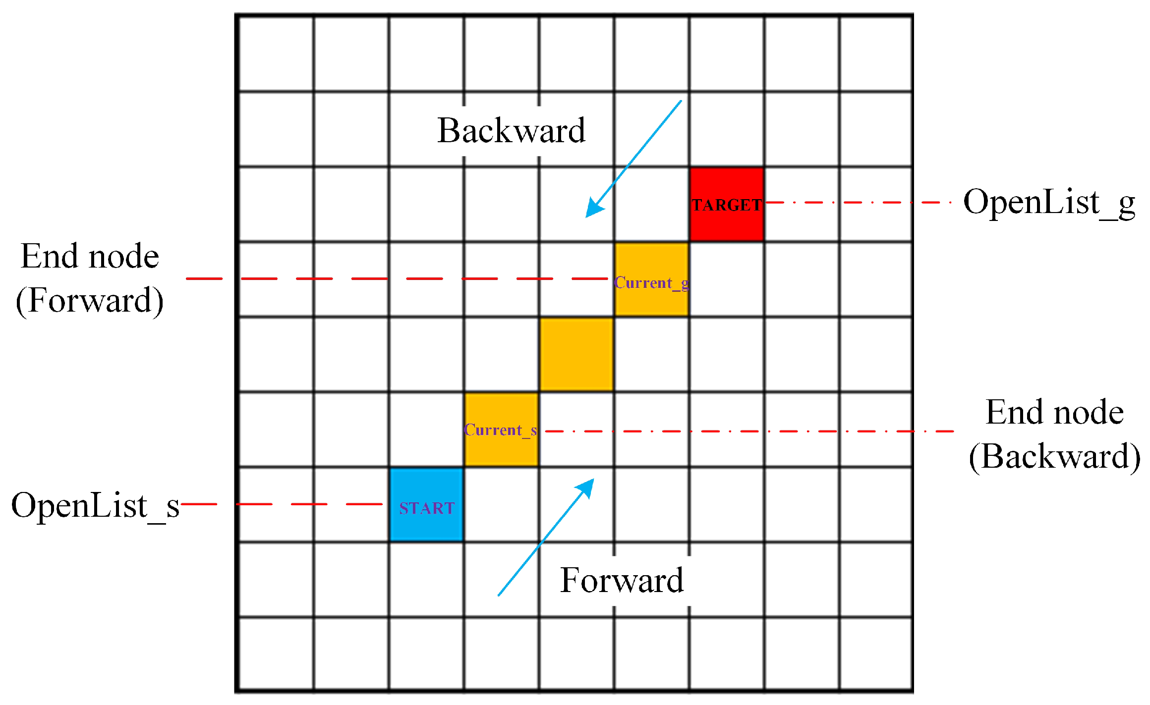
The main purpose of bidirectional A* is to take advantage of the start and goal positions to search during the path planning process. There are two OpenLists ($\mathit{OpenList\_s}$, $\mathit{OpenList\_g}$) and two CloseLists ($\mathit{CloseList\_s}$, $\mathit{CloseList\_g}$) in the bidirectional A* algorithm. As shown in Figure 2, when initializing the parameters, in the forward search direction, the START node is in the $\mathit{OpenList\_s}$, and the end node is the current node $curren{t}_g$ of the backward search direction; similarly, the GOAL node is in the $\mathit{OpenList\_g}$, and the end node is the current node $\mathit{Current\_s}$ of the forward search direction.

3.2.2. Dynamic OpenList Cost Weight Strategy for Computational Time Optimization

In the A* algorithm formula, the heuristic function can be used to choose a preferred direction for searching. So, we adjust the $H\left(n\right)$ part by introducing the weight coefficient to increase its influence and improve the calculation speed of the A* algorithm. When computing the cost of the OpenList nodes, they change gradually during the iterative process. With the increase in iterations, more and more nodes with less cost value are obtained. By considering the characteristic of the OpenList nodes’ maximum cost, minimum cost, and mean cost, we design a new weight coefficient dynamic OpenList cost weight for the path planning calculation in this study. The proposed dynamic OpenList cost weight is represented by the following formula:

$$\begin{array}{c}\hfill \left\{\begin{array}{ccc}{F}_s\left(\mathit{current\_s}\right)& =& G_s\left(\mathit{current\_s}\right)+w_{s}H\left(\mathit{current\_s}\right)\\ F_g\left(\mathit{current\_g}\right)& =& G_g\left(\mathit{current\_g}\right)+w_{g}H\left(\mathit{current\_g}\right)\end{array}\right.\end{array}$$

(5)

$$w_s=w_{min}+\frac{\left(w_{max}-w_{min}\right)\ast \left(mean\left(\mathit{OpenListcost\_s}\right)\right)}{\left(max\left(\mathit{OpenListcost\_s}\right)-min\left(\mathit{OpenListcost\_s}\right)\right)}$$

(6)

$$w_g=w_{min}+\frac{\left(w_{max}-w_{min}\right)\ast \left(mean\left(\mathit{OpenListcost\_g}\right)\right)}{\left(max\left(\mathit{OpenListcost\_g}\right)-min\left(\mathit{OpenListcost\_g}\right)\right)}$$

(7)

where $F_s\left(\mathit{current\_s}\right)$, $G_s\left(\mathit{current\_s}\right)$, and $H\left(\mathit{current\_s}\right)$ are the total cost, actual cost, and estimated cost of the $curren{t}_s$ node, respectively; similarly, $F_g\left(\mathit{current\_g}\right)$, $G_g\left(\mathit{current\_g}\right)$, and $H\left(\mathit{current\_g}\right)$ are the total cost, actual cost, and estimated cost of $\mathit{current\_g}$ node, respectively; $w_{max}$,$w_{max}$ are constant; $w_s$ represents the node’s heuristic function weight (extended from the START node); $w_g$ represents the node’s heuristic function weight (extended from the TARGET node); $\mathit{OpenListcost\_s}$ is a cost list that consists of the cost value of all the nodes (extended from the start node direction) in the $\mathit{OpenList\_s}$; $mean\left(\mathit{OpenListcost\_s}\right)$ represents the mean value of all the costs in the $\mathit{OpenListcost\_s}$, $max\left(\mathit{OpenListcost\_s}\right)$ represents the maximum value of all the costs in the $\mathit{OpenListcost\_s}$; $min\left(\mathit{OpenListcost\_s}\right)$ represents the minimum value of all the costs in the $\mathit{OpenListcost\_s}$; similarly, $\mathit{OpenListcost\_g}$ is a cost list that consists of the cost value of all the nodes (extending from the target node direction) in the $\mathit{OpenList\_g}$; $mean\left(\mathit{OpenListcost\_g}\right)$ represents the mean value of all the costs in the $\mathit{OpenList\_g}$; $max\left(\mathit{OpenListcost\_g}\right)$ represents the maximum value of all the costs in the $\mathit{OpenList\_g}$; and $min\left(\mathit{OpenListcost\_g}\right)$ represents the minimum value of all the costs in the $\mathit{OpenList\_g}$.

The weight coefficients $w_s$ and $w_g$ are dynamically changing parameters that describe the effect of $\mathit{OpenList\_s}$ nodes cost and $\mathit{OpenList\_g}$ nodes cost on heuristic function, respectively. The coefficients include the maximum, minimum, and mean costs of the OpenList nodes. The mean cost and minimum cost are also related to the process of iterations, so the heuristic part is always dynamically changing. This optimizes the computational time by efficiently adjusting the weight coefficient and guide the search toward the goal node.

When calculating the $H\left(n\right)$, the two most commonly used methods are the Manhattan distance and Euclidean distance, as shown in Formulas (8) and (9). The Euclidean distance describes the distance between two points; the Manhattan distance describes the distance between two points in the north–south direction and the distance in the east–west direction. Euclidean distance is one of the most common distance metrics, measuring the absolute distance between two positions in a multidimensional space. It is the real distance between two positions. The Manhattan distance is used to indicate the sum of the absolute wheelbases of two positions on a standard coordinate system. It only needs to be added and subtracted, which requires less computation for a large number of calculations; this eliminates the approximation in solving the square root. To reduce the computational time, in this study, we use the Manhattan distance to calculate $H\left(n\right)$.

$$H_E\left(n\right)=\sqrt{{(x_n-x_g)}^2+{(y_n-y_g)}^2}$$

(8)

$$H_M\left(n\right)=\left|x_n-x_g\right|+\left|y_n-y_g\right|$$

(9)

where $(x_n,y_n)$ is the position of the robot at the current node n; $(x_g,y_g)$ is the position of the end node.

The process of the bidirectional dynamic OpenList cost A* algorithm can be described as follows:

Step 1: Establish OpenLists and CloseLists. First, we establish two OpenLists and CloseLists for the improved algorithm: the OpenList and the CloseList. The searches from the forward search direction are defined as $\mathit{OpenList\_s}$ and $\mathit{CloseList\_s}$. Similarly, from the backward search direction; the $\mathit{OpenList\_g}$ and $\mathit{ClostList\_g}$ are also defined. Second, as shown in Figure 2, we add the START node into the $\mathit{OpenList\_s}$ and select the $\mathit{Current\_g}$ node (current node, searching from the backward search direction) as the end node. Similarly, we add the GOAL node into the $\mathit{OpenList\_g}$ and select the $\mathit{Current\_s}$ node (current node, search from the forward search direction) as the end node. We carry out the following operations on the OpenLists and ClostLists. We keep the $\mathit{ClostList\_s}$ list and $\mathit{ClostList\_g}$ empty at first.

Step 2: Parameter initialization. We define the weight coefficients of the forward search direction and backward search direction as $w_s$ and $w_g$, respectively, and assign them a value of 1 at first. We repeat steps 3–6 twice, and obtain the mean, maximum, and minimum cost values of $\mathit{OpenList\_s}$ and $\mathit{OpenList\_g}$ nodes; then, we compute $w_s$, $w_g$ by considering Formulas (6) and (7) and use them as the weight coefficients of the following calculation.

Step 3: Calculate the value of new extended nodes. We add the adjacent nodes in the forward direction into the $\mathit{OpenList\_s}$ and calculate the cost function $F\left(n\right)$ value of the newly added nodes. If the node is an obstacle grid, then we remove it from the $\mathit{OpenList\_s}$. We find the node with the minimum evaluation value in the $\mathit{OpenList\_s}$ and define it as the current node $\mathit{Current\_s}$. Next, we remove $\mathit{Current\_s}$ from the $\mathit{OpenList\_s}$ and transfer it into the $\mathit{ClostList\_s}$. We carry out the same operations on the adjacent nodes in the backward direction. Then, we update the $\mathit{OpenList\_g}$ and $\mathit{ClostList\_g}$.

Step 4: Define the parent node. We set the adjacent nodes of the current node in the forward direction. These are not placed in the $\mathit{ClostList\_s}$ or into the $\mathit{OpenList\_s}$. We use the current node in the forward direction as the parent node of the newly added nodes in the forward direction. We conduct the same operations on the adjacent nodes in the backward direction.

Step 5: Judge and update the newly added nodes $F\left(n\right)$ and $G\left(n\right)$ values. First, we check if the newly added nodes in the forward direction obtained in Step 3 already exist in the $\mathit{OpenList\_s}$. If the nodes do not exist in the $\mathit{OpenList\_s}$, then we use the current node as the parent node of the newly added nodes. If the nodes are in the $\mathit{OpenList\_s}$, then we compare their $G\left(n\right)$ values. If the newly added node’s value is smaller, we use the current node as the parent node of the newly added nodes and update the newly added node’s $F\left(n\right)$ value. We carry out the same operations on the adjacent nodes in the backward direction and update the parent node of the newly added nodes in the backward direction.

Step 6: Judge the loop exit condition. We judge whether the $\mathit{OpenList\_s}$ is empty or not. If the $\mathit{OpenList\_s}$ is empty, all of the operations will stop; otherwise, we judge whether $\mathit{Openlist\_s}$ and $\mathit{Openlist\_g}$ have the same nodes. If so, then we calculate the $F\left(n\right)$ value of all the same nodes and select the node with the smallest value as the intersection node of $\mathit{Openlist\_s}$ (forward search) and $\mathit{Openlist\_g}$ (backward search). We obtain the path from the GOAL node, move forward to the intersection node, and finally reach the START node. Otherwise, we continue to calculate the cost of the extended nodes that search from the forward search direction. We carry out the same operations on the $\mathit{OpenList\_g}$.

As described above, in Step 1, the $\mathit{Current\_g}$ node and $\mathit{Current\_s}$ node were obtained from the iterative process. We needed to consider the initialization of the end node in both the forward direction and the backward direction. During initialization, we selected the GOAL node as the end node of the $\mathit{Current\_s}$ node and the START node as the end node of the $\mathit{Current\_g}$ node. Furthermore, to facilitate the calculation of the weight coefficient, as described in step 2, we first assigned the two weight coefficients of the heuristic function of the bidirectional search a value of 1. Thus, we obtained the initial cost of nodes in the $\mathit{OpenList\_s}$ and $\mathit{OpenList\_g}$. Finally, the dynamic OpenList cost weight coefficients $w_s$, $w_g$ were obtained; we could use these to calculate the cost value of $F\left(n\right)$ later.

3.3. Simulation Results and Analysis of the Computational Time Optimization Strategy

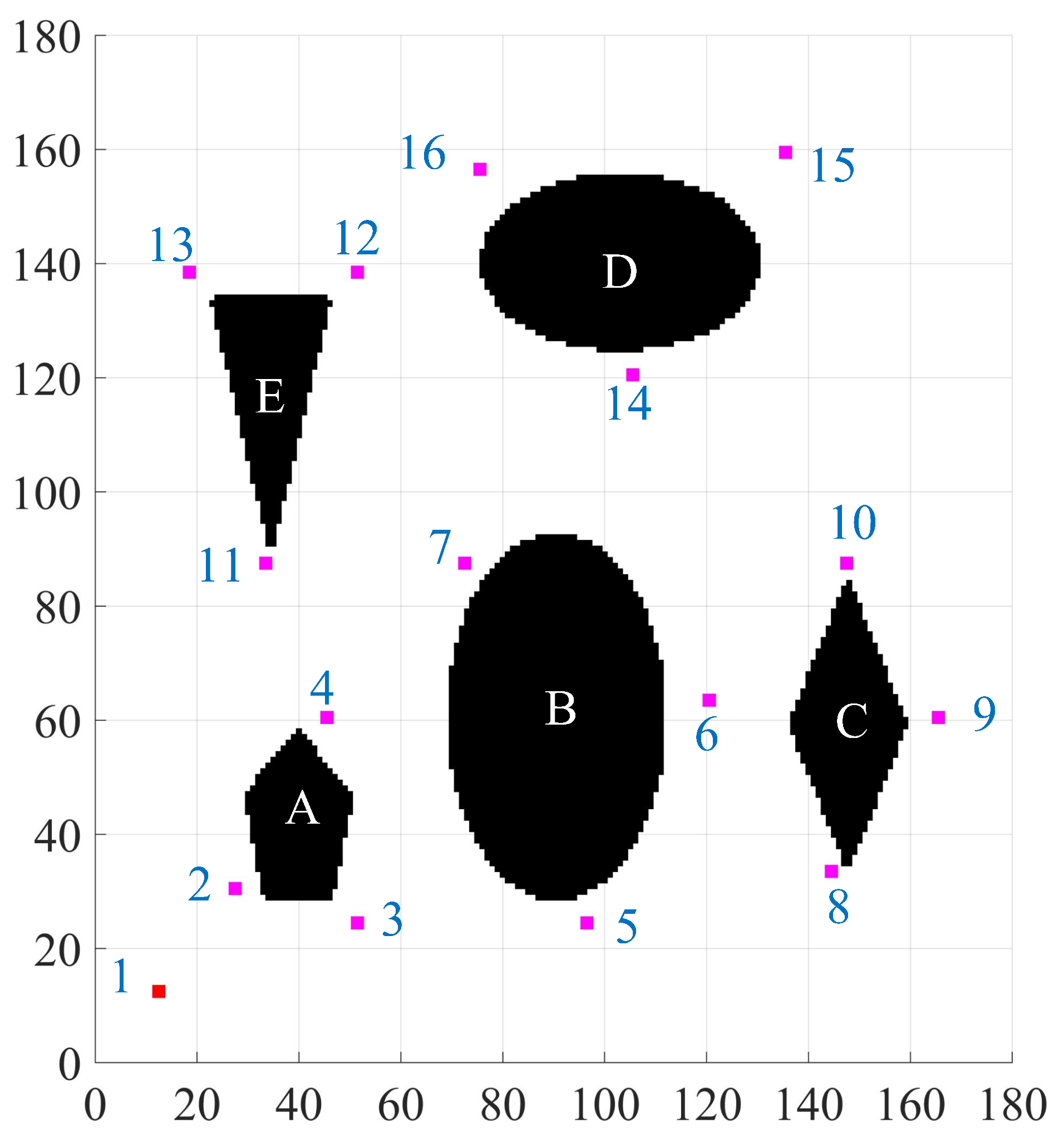
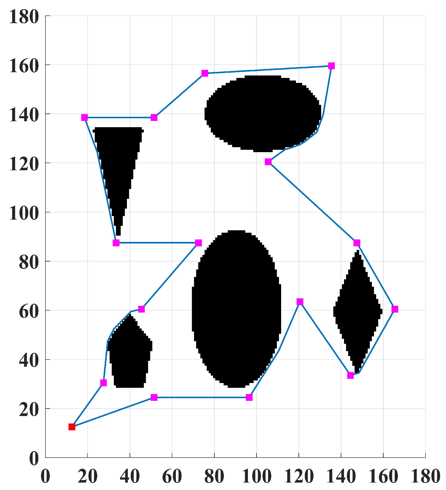
In this study, an Intel(R) Core (TM) i5-5200U CPU @ 2.20 GHz, RAM 16 GB, with a Windows 10 Education 64 operating system, was used for experimental simulation. The coordinates of the start position were (12, 12), and the coordinates from goal position 1 to 15 in Figure 1 are (27, 30), (51, 24), (45, 60), (96, 24), (120, 63), (72, 87), (144 33), (165, 60), (147, 87), (33 87), (51,138), (18,138), (105,120), (135, 159), and (75,156). To verify the efficiency of the bidirectional dynamic OpenList cost weight A* algorithm, some comparative simulations were designed. We compared the weighted bidirectional improved A* algorithm with traditional A* and discussed the effects of different weight coefficients and the resolution on the computation time. To ensure the accuracy of the simulation results, we designed and repeated the algorithm 30 times.

As shown in

Table 1. Simulation comparison results of traditional A* algorithm and bidirectional dynamic OpenList cost weight A* algorithm regarding average computation time.

Resolution	Traditional A* Algorithm(s)	Bidirectional Dynamic OpenList Cost Weight A* Algorithm(s)
$120\times 120$	79.50	26.39
$180\times 180$	250.91	50.27
$240\times 240$	628.53	83.36

, compared with the traditional A* algorithm, the computation time of the bidirectional dynamic OpenList cost weight A* algorithm is significantly shorter. As the resolution of the environment map changes from $120\times 120$ to $180\times 180$ and $120\times 120$ to $240\times 240$, the calculation time’s multiples of the traditional A* algorithm and the bidirectional dynamic OpenList cost weight A* algorithm are 3.16 (250.91:79.50), 7.91 (628.53:79.50) and 1.90 (50.27:26.39), 3.16 (83.36:26.39), respectively. The multiple increases in the calculation time of the algorithm are significantly less than those of the traditional A* algorithm.

To further verify the effectiveness of the bidirectional dynamic OpenList cost weight A* algorithm, we introduced constant weight w = 1, 1.5, 2, and five other weight coefficients for comparison. The formulas of the five weight coefficient functions ($w_1,w_2,w_3,w_4,w_5$) are described in Formulas (10)–(14):

$$w_1:w_k=w_{\min }+\frac{(w_{\max }-w_{min})}{(1-\frac{k}{{\mathrm{Est}}_{iter}})}$$

(10)

$$w_2:w_k=w_{min}+(w_{max}-w_{min}){(\frac{k}{{\mathrm{Est}}_{iter}})}^2$$

(11)

$$w_3:w_k=w_{\min }+(w_{max}-w_{min})\left[\frac{2k}{{\mathrm{Est}}_{iter}}-{(\frac{k}{{\mathrm{Est}}_{iter}})}^2\right]$$

(12)

$$w_4:w_k=w_{min}{\left(\frac{w_{min}}{w_{max}}\right)}^{\frac{1}{\left(1+\frac{ck}{{\mathrm{Est}}_{iter}}\right)}}$$

(13)

$$w_5:w_k=w_{min}+\frac{(w_{\max }-w_{min})}{\sqrt{2\pi }{e}^{\left[\frac{-{\left(\frac{k}{{\mathrm{Est}}_{iter}}\right)}^2}{2}\right]}}$$

(14)

where k represents the kth iteration; $w_k$ represents the weight coefficient of the kth iteration; $w_{end}$, $w_{start}$, and c are constants; $Es{t}_{iter}$ represents the pre-estimated maximum number of iterations’ and e is the Euler number.

The parameter $Es{t}_{iter}$ in the five functions are obtained by calculating the $H\left(n\right)$ value, which evaluates from the start node to the end node. The constant c in the coefficient $w_4$ is 1. Constant $w_{min}$ is 1, and $w_{max}$ is 2. The e coefficient $w_4$ is 1. Constant $w_{min}$ is 1 and $w_{max}$ is 2.

The results of $w_1-w_5$ and w = 1, 1.5, 2 are based on a bidirectional search. As can be seen from

Table 2. Simulation comparison results of different weights of coefficients on average computational time.

Resolution	w = 1 (s)	w = 1.5 (s)	w = 2 (s)	Bidirectional Dynamic OpenList Cost Weight A* Algorithm (s)	${\mathit{w}}_1$ (s)	${\mathit{w}}_2$ (s)	${\mathit{w}}_3$ (s)	${\mathit{w}}_4$ (s)	${\mathit{w}}_5$ (s)
$180\times 180$	106.35	56.76	53.03	50.27	60.83	66.15	56.95	631.14	65.93

, the dynamic OpenList cost weight A* algorithm shows better performance than any other weight coefficient in terms of calculation time.

3.4. Strategies of Improved A* Algorithm for the Shortest Distance between Any Two Points

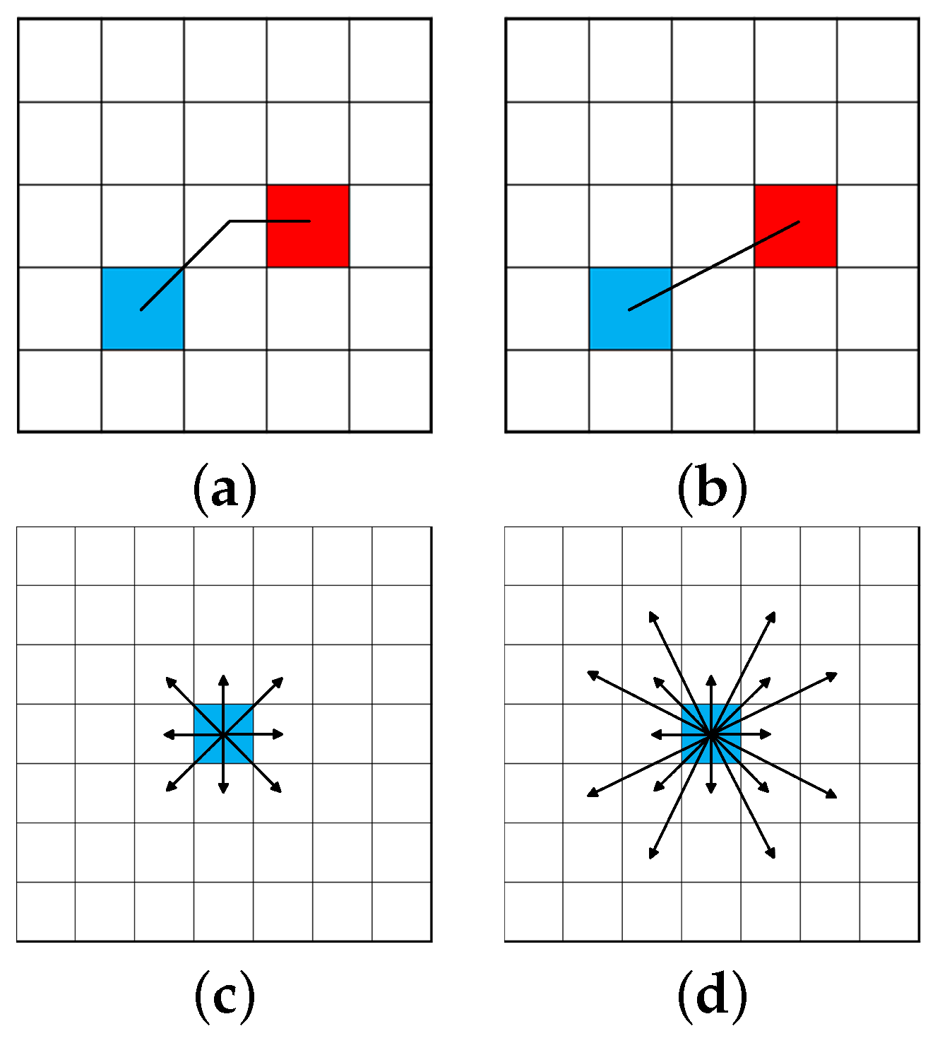
Although the collision-free path can be obtained by using the traditional eight-adjacent nodes A* algorithm, there are many inflection nodes and repeated calculations, and sometimes the path distance is long. Thus, it is necessary to reduce the inflection nodes and shorten the path distance for path planning. To solve this problem, we changed the expansion node number from 8 to 16.

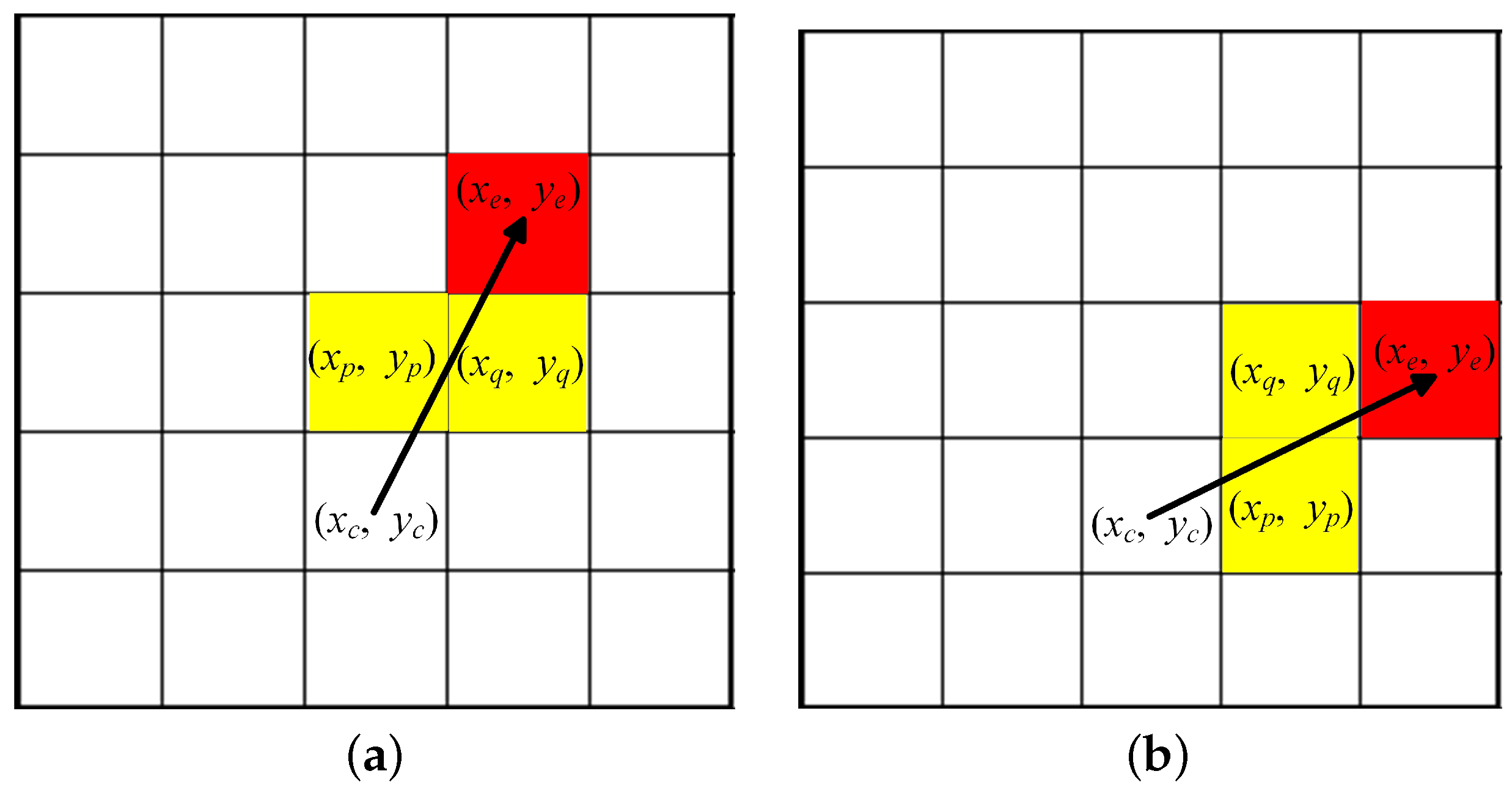
As shown in Figure 3, the 16 adjacent nodes search method can lead the search to the goal node (red node in Figure 3 directly), which significantly reduces the path length and the number of nodes. However, the 16 adjacent nodes strategy also introduces more nodes that must be evaluated to determine whether they are an obstacle or not. For example, in Figure 4, node P $(x_p,y_p)$ and node Q $(x_q,y_q)$ are the waypoints, and node E $(x_e,y_e)$ is the expansion node; before adding the extend nodes into $\mathit{OpenList\_s}$ or $\mathit{OpenList\_g}$, it is necessary to judge whether the three nodes (P, Q, and E) are obstacles or not. The relationship between the waypoints, current node C $(x_c,y_c)$, and next node E $(x_e,y_e)$ in the coordinates are:

The obstacle judgment formula is:

$$\begin{array}{c}\hfill \left\{\begin{array}{ccc}{x}_p& =& x_c\\ y_p& =& \frac{y_c+y_e}{2}\\ x_q& =& x_e\\ y_q& =& \frac{y_c+y_e}{2}\end{array}\right.\end{array}$$

(15)

When node P and node Q are above or at the bottom of node C, the relationships between the extended node and the waypoints are as shown in Formula (15), where ($x_e$, $y_e$), ($x_p$, $y_p$), ($x_q$, $y_q$), ($x_c$, $y_c$) are the coordinates of node E, node P, node Q, and node C in the Cartesian coordinate system, respectively. By using the proposed obstacle judgment formula method, we more accurately judge whether the new expansion point is an obstacle or not than is possible with many other methods, such as selecting the sample points in the path to judge whether the sample point is in the obstacle or not. When node P and node Q are to the left or to the right of node C, the relationship between the extended node and the waypoints is as shown in Formula (16):

$$\begin{array}{c}\hfill \left\{\begin{array}{ccc}{x}_p& =& \frac{x_c+x_e}{2}\\ y_p& =& y_c\\ x_q& =& \frac{x_c+x_e}{2}\\ y_q& =& y_e\end{array}\right.\end{array}$$

(16)

3.5. Simulation Results and Analysis of the Shortest Distance of the Path Planning Improved Strategy

To optimize the path planning and compare the performance of the shortest distance path planning strategy, we compared the 8 adjacent nodes and the 16 adjacent nodes using the improved bidirectional weight A* algorithm mentioned above.

Table 3. The shortest distance between any two points of the 8-neighborhood method.

	1 (Initial Point)	2	3	4	5	6	7	8	9	10	11	12	13	14	15	16
1
2	22.21
3	42.968	24.484
4	66.146	40.694	38.968
5	86.968	70.484	44	64.904
6	136.63	161.98	104.77	117.216	47.936
7	103.496	79.458	70.694	36.764	81.592	68.49
8	138.694	118.726	95.726	127.426	49.726	37.936	160.566
9	179.63	159.42	145.356	156.872	93.802	73.834	114.318	37.28
10	228.196	190.674	187.604	131.254	83.114	35.936	78.968	60.694	33.452
11	82.694	59.312	86.834	30.968	92.77	114.942	38	174.26	162.426	116.968
12	142.63	117.592	112	78.484	139.458	101.738	58.694	141.26	148.98	115.114	57.452
13	126.484	109.726	134.28	87.178	148.98	162.184	118.7	201.464	211.668	186.082	56.21	32
14	149.33	124.292	119.012	82.012	107.662	62.21	45.248	102.146	87.528	53.662	83.662	59.452	141.77
15	230.744	205.706	201.598	178.846	158.426	103.522	161.05	131.038	110.42	74.968	146.636	96.662	128.662	59.42
16	170.566	145.528	139.936	106.42	153.318	165.808	69.242	196.05	168.808	148.222	85.388	29.452	63.452	59.592	59.242

and

Table 4. The shortest distance between any two points of 16-neighborhood strategy.

	1 (Initial Point)	2	3	4	5	6	7	8	9	10	11	12	13	14	15	16
1
2	22.21
3	38.14	24.484
4	60.662	34.038	37.968
5	80.968	67.656	42	60.904
6	124.7	96.35	73.388	87.802	33.936
7	92.974	66.974	61.382	27.866	73.108	66.076
8	128.694	115.312	86.898	96.458	46.484	33.038	116.324
9	151.942	151.324	103.974	139.458	71.006	57.006	93.248	24.624
10	124.776	155.776	85.598	104.356	68.146	30.624	71.968	51.108	25.038
11	79.796	55.312	71.834	24.14	65.802	99.044	38	133.222	147.528	106.14
12	130.388	99.936	112	75.656	122.42	79.528	49.038	113.082	121.044	100.076	47.452
13	125.656	108.898	121.038	75.108	119.942	127.458	84.458	156.98	159.012	139.184	46.554	32
14	117.496	93.942	88.458	55.732	91.764	58.554	30.694	85.592	66.076	37.522	70.694	59.038	114.356
15	213.738	144.432	134.566	92.254	130.592	91.968	73.216	124.14	93.178	69.312	118.044	89.662	121.662	46.108
16	157.388	114.974	130.21	90.28	128.662	130.808	66.828	157.91	136.292	123.636	66.42	22.554	56.554	48.522	57.242

are the path length matrix of the 8 neighborhood and 16 neighborhood, respectively. In the tables, the number in row i, column j represents the shortest distance from point i to point j. For example, the shortest distance from point 3 to point 1 in Table 3 is the number in row 3 column 1; that is, 42.968.

Table 5. The shortest distance between any two points.

	1 (Initial Point)	2	3	4	5	6	7	8	9	10	11	12	13	14	15	16
1	0	22.21	38.14	60.662	80.968	124.7	92.974	128.694	151.942	124.776	79.796	130.388	125.656	117.496	213.738	157.388
2	22.21	0	24.484	34.038	67.656	96.35	66.974	115.312	151.324	155.776	55.312	99.936	108.898	93.942	144.432	114.974
3	38.14	24.484	0	37.968	42	73.388	61.382	86.898	103.974	85.598	71.834	112	121.038	88.458	134.566	130.21
4	60.662	34.038	37.968	0	60.904	87.802	27.866	96.458	139.458	104.356	24.14	75.656	75.108	55.732	92.254	90.28
5	80.968	67.656	42	60.904	0	33.936	73.108	46.484	71.006	68.146	65.802	122.42	119.942	91.764	130.592	128.662
6	124.7	96.35	73.388	87.802	33.936	0	66.076	33.038	57.006	30.624	99.044	79.528	127.458	58.554	91.968	130.808
7	92.974	66.974	61.382	27.866	73.108	66.076	0	116.324	93.248	71.968	38	49.038	84.458	30.694	73.216	66.828
8	128.694	115.312	86.898	96.458	46.484	33.038	116.324	0	24.624	51.108	133.222	113.082	156.98	85.592	124.14	157.91
9	151.942	151.324	103.974	139.458	71.006	57.006	93.248	24.624	0	25.038	147.528	121.044	159.012	66.076	93.178	136.292
10	124.776	155.776	85.598	104.356	68.146	30.624	71.968	51.108	25.038	0	106.14	100.076	139.184	37.522	69.312	123.636
11	79.796	55.312	71.834	24.14	65.802	99.044	38	133.222	147.528	106.14	0	47.452	46.554	70.694	118.044	66.42
12	130.388	99.936	112	75.656	122.42	79.528	49.038	113.082	121.044	100.076	47.452	0	32	59.038	89.662	22.554
13	125.656	108.898	121.038	75.108	119.942	127.458	84.458	156.98	159.012	139.184	46.554	32	0	114.356	121.662	56.554
14	117.496	93.942	88.458	55.732	91.764	58.554	30.694	85.592	66.076	37.522	70.694	59.038	114.356	0	46.108	48.522
15	213.738	144.432	134.566	92.254	130.592	91.968	73.216	124.14	93.178	69.312	118.044	89.662	121.662	46.108	0	57.242
16	157.388	114.974	130.21	90.28	128.662	130.808	66.828	157.91	136.292	123.636	66.42	22.554	56.554	48.522	57.242	0

is the path length matrix composed of the minimum length of the 8 neighborhood (Table 3) and the 16 neighborhood (Table 4). For example, the shortest distance from point 3 to point 1 in Table 3 is 42.968; in Table 4, it is 38.14; and so, in Table 5, the shortest distance from point 3 to point 1 is 38.14. This is due to the distance matrix being symmetric, simultaneously allowing us to effectively solve the proposed problem. We can obtain a complete distance matrix of any two points, as shown in Table 5.

The total positions number for path planning is 16, so we obtain a $16\times 16$ integer distance matrix as the distance matrix is symmetrical; that is, the distance from one position to the other is equal to the distance from the other to the position. In Table 3 and Table 4, we only show the partial distance for a better comparison of the distance value between any two positions; the distance number between all of the 16 nodes is 120. As shown in

Table 6. Comparing the results of the 8 adjacent nodes and 16 adjacent nodes’ path lengths.

	The 16 Adjacent Nodes Path Length Is Shorter	The Path Lengths Are Equal	The 8 Adjacent Nodes Path Length Is Shorter
Number	115	5	0

, compared with the path length generated by using 8 adjacent nodes, the 16 adjacent nodes A* algorithm shows better performance, and all of the generated path lengths are less than or equal to the 8 adjacent nodes A* algorithm for the redundant points are removed.

To further verify the performance of bidirectional dynamic weighted-A* algorithm, we compared the improved A* algorithm with goal-oriented rapidly exploring random tree (GORRT) [38] algorithm, where the step size of GORRT is eight, and the threshold is five. If nodes were closer than this, they were taken as almost the same. So, the shortest distance between of any two nodes by using GORRT are shown in

Table 7. The shortest distance between any two nodes obtained using GORRT.

	1 (Initial Point)	2	3	4	5	6	7	8	9	10	11	12	13	14	15	16
1
2	26.342
3	68.397	28.399
4	95.557	58.038	41.884
5	109.377	99.535	59.763	76.168
6	153.777	130.836	106.117	130.889	57.971
7	120.788	116.53	75.654	60.48	99.202	75.407
8	175.884	171.403	123.506	133.552	68.795	50.6	157.141
9	222.912	188.225	174.266	181.991	106.044	98.66	131.962	67.721
10	221.069	229.089	188.874	155.367	107.134	42.562	107.568	83.22	36.372
11	100.864	67.435	101.057	57.949	140.626	129.746	49.095	211.729	253.191	149.308
12	204.597	187.866	153.494	97.746	179.677	150.481	83.997	201.065	213.031	166.08	80.975
13	156.989	123.806	169.62	116.288	164.781	196.576	105.162	223.524	247.17	171.414	59.646	59.319
14	174.623	175.014	170.507	107.231	155.634	76.445	51.626	117.39	195.725	77.426	133.163	82.739	114.089
15	257.273	261.045	234.944	179.128	181.176	123.227	147.694	157.193	115.667	92.181	171.403	106.334	147.733	65.716
16	234.244	165.681	208.532	123.691	179.6	149.971	83.888	182.017	195.789	155.005	104.488	51.061	93.717	66.988	69.66

.

By analyzing the results of the16 adjacent nodes (Table 4) and GORRT’s path length (Table 7), we also obtained the comparison results of the 16 adjacent nodes and GORRT’s path length. The results are shown in

Table 8. Comparing the results of the 16 adjacent nodes and GORRT path lengths.

	16 Adjacent Nodes Path Length Is Shorter	Path Lengths Are Equal	GORRT Path Length Is Shorter
Number	119	0	1

. The path length generated by using 16 adjacent nodes also produced better performance with 199 path lengths being shorter and 1 path length being longer.

4. LM-SSPSO Algorithm for Traversing Multiple Goal Positions

As mentioned above, we obtained the shortest distance of any two positions of the 16 nodes (including the start position). The next step was to find the shortest path for traversing all suspicious positions just once. The process is similar to that of the traditional trade salesperson problem (TSP) [39]: the distance from position P to position Q is equal to that from position Q to position P. Thus, in this section, we solve the multiple goal positions path planning problem by considering the methods of solving the TSP. To solve the TSP, many algorithms have been studied, such as the greedy algorithm, genetic algorithm (GA), particle swarm optimization (PSO), harmony search (HS), etc. Refael Hassin and Ariel Keinan [40] proposed greedy heuristics with regret as the cheapest insertion method for solving the TSP. They improve the Greedy algorithm by allowing partial regret. The computational results showed that the relative error is reduced and the computational time is quite short. Urszula Boryczka and Krzysztof Szwarc [41] studied an improved HS algorithm to solve the TSP. The results showed that the proposed algorithm has a significant effect and that the summary average error can be effectively reduced. An initial population strategy (KIP, k-means initial population) was applied by Yong Deng et al. [42]. The information to improve the GA, helping to find the optimal solution for the TSP. Fourteen TSP examples were used to test the algorithm, and the results showed that the KIP strategy can effectively decrease the best error value. Matthias Hoffmann et al. [43] presented a discrete PSO algorithm used to solve the TSP, which provides insight into the convergence behavior of the swarm. The method is based on edge exchanges and combines differences by computing their centroid. The method was compared with other approaches; the evaluation result showed that the proposed edge-exchange-based PSO algorithm performs better than the traditional approaches. Although many traditional algorithms have been used to solve the TSP, each of the above approaches has its limitations. For example, the diversity of PSO is easily lost during iteration. The greedy algorithm and HS algorithm may fall into a local optimum, and the result of GA strongly depends on the initial value. So, we introduced the LM-SSPSO algorithm to improve the efficiency of EOD robot path planning.

4.1. Mathematical Model of Multiple Goal Positions Path Planning

In this subsection, we present the path planning for the EOD robot for the multiple-goal positions mathematical model. The aim of our research was to find the shortest path that allows all goal positions to be traversed just once, followed by a return to the start position. So, we developed the mathematical solution with reference to the methods of solving the TSP. We define the path planning problem as an instance $L=(n,dist)$ of multiple goal positions $\{1,\dots ,n\}$, so we obtain an $n\times n$ integer distance matrix of all the goal positions. The path to be optimized can be described as a permutation D of the multiple goal positions, where $D\left(i\right)$ denotes the ith visited goal positions. Hence, the formula of the total distance $L=(n,dist)$ is:

$$L=\underset{D\in \mathrm{Rn}}{argmin}\left({\mathrm{dist}}_{\mathrm{D}\left(\mathrm{n}\right),\mathrm{D}\left(1\right)}+\sum _{1\le i\le n-1}{\mathrm{dist}}_{\mathrm{D}\left(i\right),\mathrm{D}\left(i+1\right)}\right)$$

(17)

where Rn is the symmetric group on $\{1,\cdots ,n\}$, $dis{t}_{D\left(i\right),D(i+1)}$ denotes the distance between the ith goal position and the $(i+1)$th goal position, and $dis{t}_{D\left(n\right),D\left(1\right)}$ denotes the distance between the nth goal position and the start position.

4.2. Traditional PSO Algorithm

The PSO algorithm is a population-based metaheuristic algorithm that is widely used for its powerful control parameters; it is also easy to apply. It is inspired by the social behavior of bird flocks. When birds move in a group, each bird can be regarded as one particle, and all the particles form a swarm $S=(s_1,s_2,\dots ,s_i,\dots ,s_N)$, where N is the population size of the swarm. Each bird has its own velocity and position. The velocity of particle i is represented as $V_i=(v_{i1},v_{i2},\dots ,v_{id},\dots ,v_{iDm})$, where d is the dimension. The position of particle i is represented as $X_i=(x_{i1},x_{i2},\dots ,x_{id},\dots ,x_{iDm})$. As time advances, the particles update their velocity and position with mutual coordination and information-sharing mechanisms. The particles obtain the best position by constantly updating their individual optimal positions and swarm optimal positions. The best position of an individual particle i is represented as $pbes{t}_i=(p_{i1},p_{i2},\dots ,p_{id},\dots ,p_{iDm})$. The best position of the swarm is represented as $gbest=(g_1,g_2,\dots ,g_d,\dots ,g_{Dm})$. The positions and velocities of each particle are updated as follows:

$$\left\{\begin{array}{c}v{}_{id}^{k+1}=wv{}_{id}^k+c_1{r}_1(pbes{t}_{id}-x_{id}^k)+c_2{r}_2(gbes{t}_d-x_{id}^k)\hfill \\ x_{id}^{k+1}=x_{id}^k+v{}_{id}^{k+1}\hfill \end{array}\right.$$

(18)

where Dm represents the maximum dimension of the particle; $v{}_{id}^k$ and $v{}_{id}^{k+1}$ represent the d-dimension element of the current velocity and new velocity of the particle, respectively; $x_{id}^k$ and $x_{id}^{k+1}$ represent the d-dimension element of the current position and new position of the particle, respectively; w represents the weight coefficient; i represents the particle number; k and $k+1$ represent the kth and $(k+1)$th iteration, respectively; $c_1$ and $c_2$ are positive acceleration constants and scale the contribution of cognitive and social components, respectively; $r_1$ and $r_2$ represent uniform random variables between (0, 1); $pbes{t}_{id}$ represents the dth element of the particle i’s best individual position; and $gbes{t}_d$ represents the dth element of the swarm’s global (swarm) best position. In the PSO algorithm, each particle is attracted by two positions: the global best position and its previous best position. 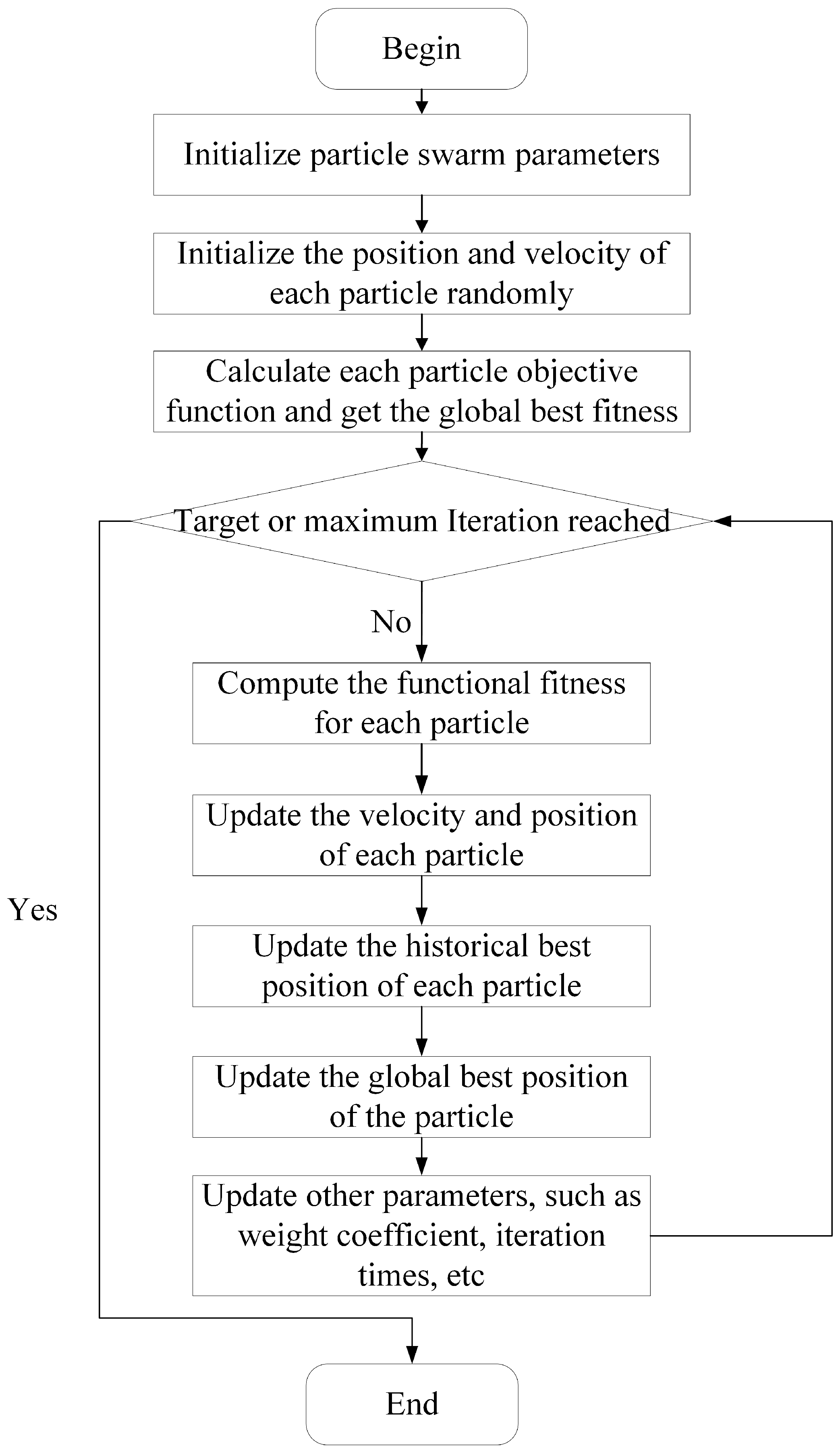During iterations, the particles adjust their positions and velocities according to Formula (18), and the flowchart of the traditional PSO algorithm shown in Figure 5; when the algorithm achieves the goal or reaches the maximum iteration, the search stops. The application of PSO in path planning has been explored in various studies. In the following section, we provide a hybrid algorithm that shows fast convergence and addresses diversity in solving optimization problems.

4.3. Improved Strategies for Planning the Shortest Distance of Traversing All Goal Positions

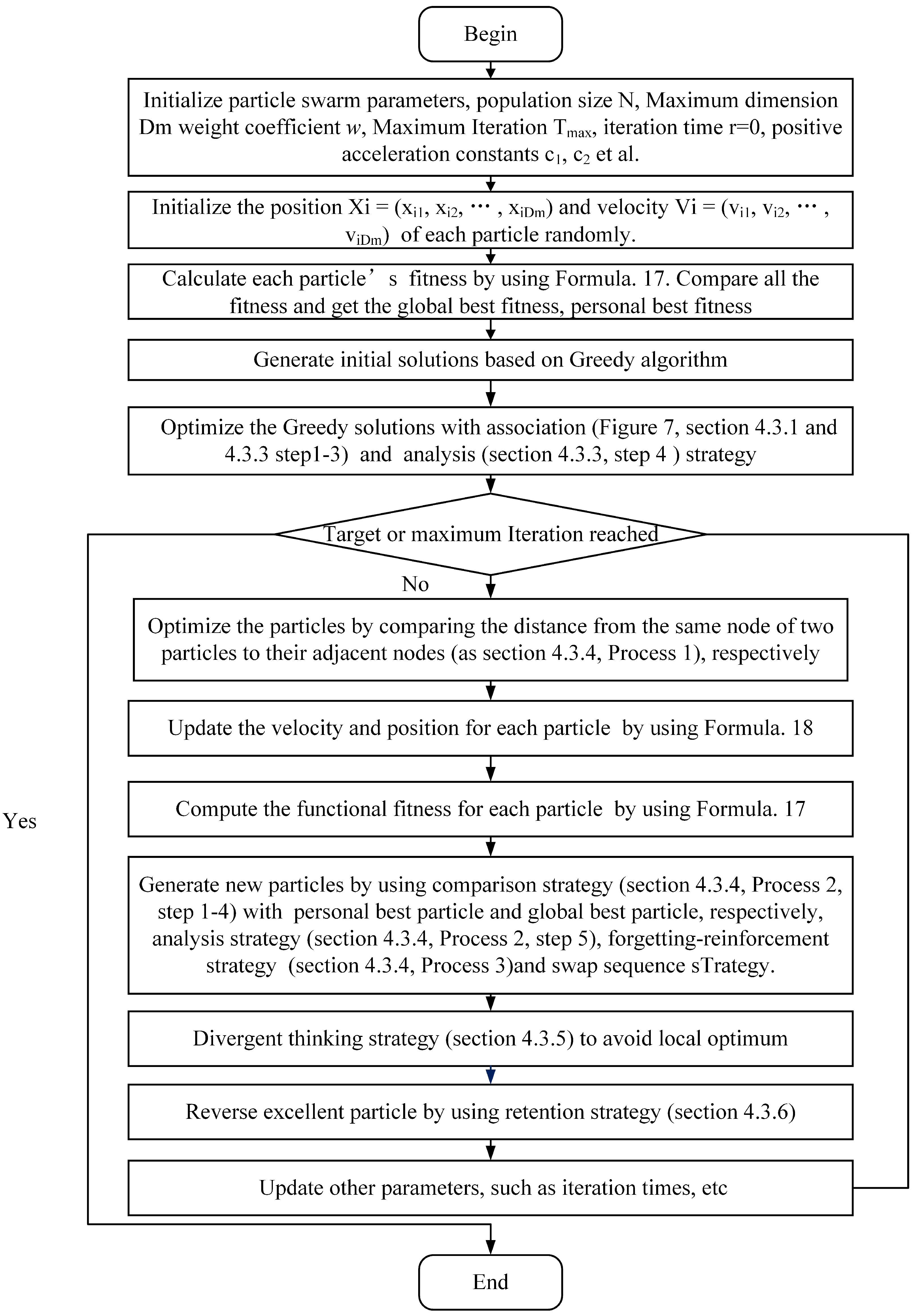
The PSO algorithm is widely used due to its simple operation, easy implementation, and fast speed. However, it still has some shortcomings, such as the results depending on the initial solution, and the lack of randomness in particle position changes, so the diversity of the particles may reduce and fall into a local optimum during iteration. To overcome the drawbacks, we improve the traditional PSO with the following strategies. First, a greedy algorithm and an association strategy are introduced to optimize initial solutions. In addition, forgetting–reinforcement, comparison, analysis strategies, and divergent thinking are proposed to maintain the diversity of the swarm, avoid the local optimum, and obtain better solutions. The forgetting–reinforcement strategy is used to update the particle in the swarm or to randomly generate a new particle under certain conditions, the comparison strategy is used to optimize the individual particle, and the analysis strategy is used to generate a new particle from two particles. Furthermore, a divergent thinking strategy is introduced to increase the randomness of the particles. Finally, the retention strategy is used to reserve a better solution in the swarm for the next iteration. The flowchart of the LM-SSPSO algorithm is presented in Figure 6.

Compared with the traditional PSO algorithm, there are four aspects in which the LM-SSPSO algorithm provides optimization. Firstly, the initial solutions are optimized; by using the greedy algorithm and analyze strategy, the quality of initial solution can be effectively improved. Then, two different particles are optimized by considering the distance of the same node to their adjacent nodes with the compare strategy. Meanwhile, the personal best particle and global best particle are also used to provide path points to optimize the particle. Additionally, the particle is optimized with analysis strategy the swaps two randomly different position in one particle. The swap sequence strategy is also introduced to update the particle by using new swap operators, which include new position and velocity update formulas. Whether the swap sequence strategy is used or not depends on the forgetting–reinforcement strategy. Finally, to avoid the local optimum, the divergent thinking strategy is also used to optimize the particle with the worst particle and select the better particle with the retention strategy in the end. The detailed description of each strategy is introduced in the following section.

4.3.1. The LM-SSPSO-Based Method to Traverse All Goal Positions

Inspired by the behaviors of learning and memory, we propose a novel intelligent algorithm called LM-SSPSO. In the improved algorithm, we introduce several strategies to solve the multiple goal positions path planning problem. When people learn and memorize information, they often forget or confuse similar knowledge. To solve problems, people can compare and analyze specific features, associate the information with a similar object, and combine divergent thinking to enhance memory, etc. For example, if someone confuses the words “dessert”, “desert”, and “dissert”, they can compare the differences: “d-es-sert”, “d-e-sert”, and “d-is-sert”. The middle letters are different in the three words. The flowchart of LM-SSPSO is shown in Figure 6. It includes the process of association, comparison, analysis, forgetting–reinforcement, divergent thinking, and retention.

Association means that one concept leads to other related concepts; the origin of association can be a geometric figure, such as the behaviors of animals or social behaviors, etc. The results are the operations with similar behaviors in the swarm. In the LM-SSPSO algorithm, the operations of association can be described as selecting a group of particles from the swarm and then referring to a feature or figure, for example, a triangle. The sequences of the corresponding nodes are swapped for each particle. Figure 7 shows the process of association; the node on the hypotenuse is swapped with that on the right-angled side. The operations are detailed in the following section.

Comparison is the act of distinguishing or finding the differences between two or more objects and obtaining a better final result. In LM-SSPSO, a comparison strategy is usually applied to two objects, and the strategy obtains a desirable solution according to a certain rule. There are two methods of comparison. One involves comparing the distance from the same node of two particles to their adjacent nodes, and the other involves comparing the distance of a partial optimization particle with that of an unprocessed particle. Partial optimization includes selecting a segment from one particle, deleting the nodes that are the same as the segment in another particle, and adding the selected segment to the end of another particle.

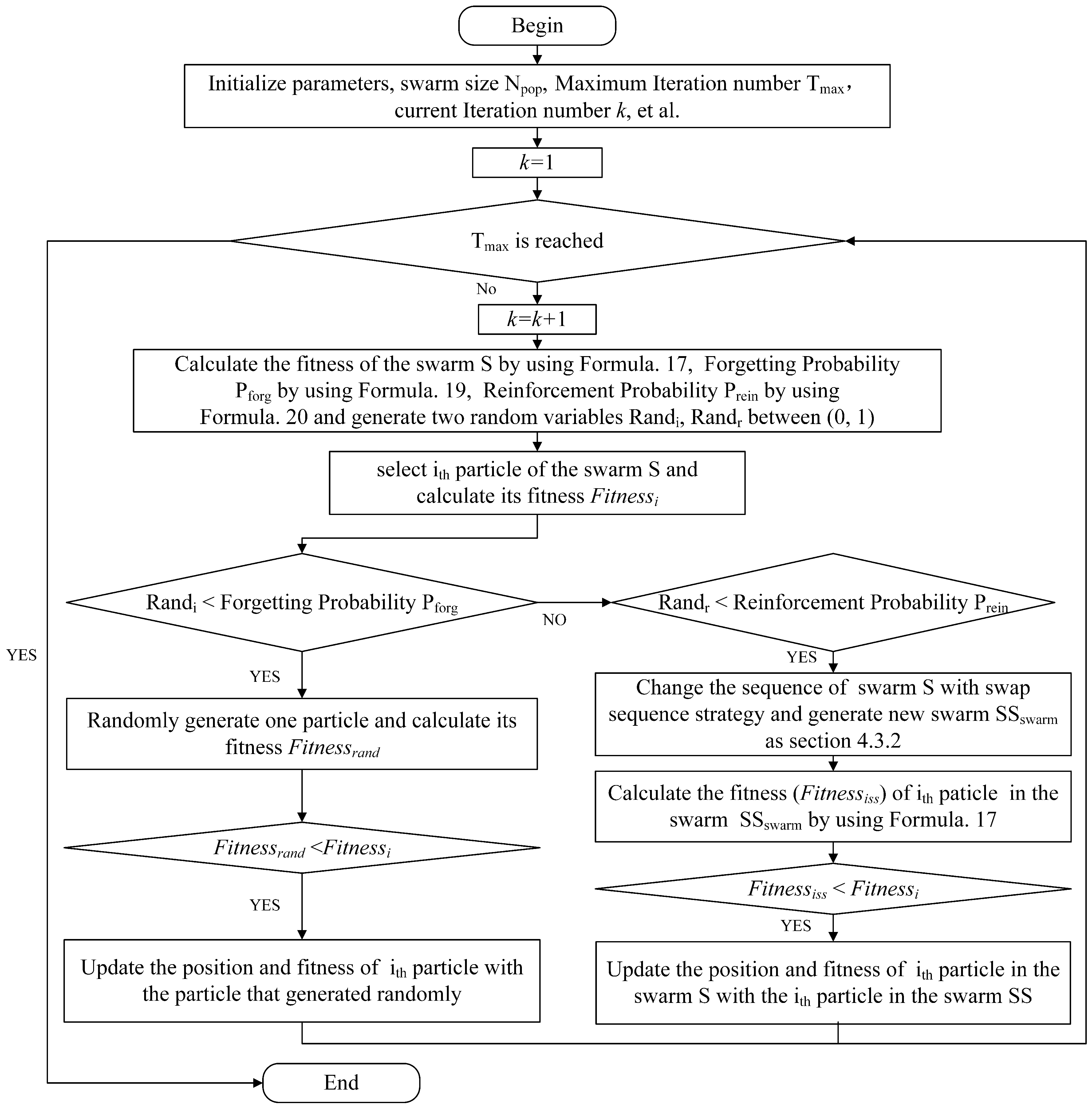
Forgetting [44] is a special function in the human brain, which means the things that are experienced no longer remain in the memory. This behavior may involve the random loss or removal of information. Reinforcing is the opposite of forgetting; it is a way to consolidate information firmly. The proposed forgetting–reinforcement strategy imitates the behaviors of people forgetting information and strengthening their memories. This can lead to the loss of some or all of the information in one particle to avoid local optima and to generate new particles to maintain the diversity of the swarm. In the LM-SSPSO, a forget probability function and a reinforcement probability function are introduced to increase the diversity of the swarm. The flowchart of the forgetting–reinforcement strategy is shown in Figure 8, and the forgetting probability formula and reinforcement probability formula are described in Formulas (19) and (20), respectively.

The forgetting–reinforcement strategy is applied after the analysis strategy of LM-SSPSO, as shown in Figure 6. It generates a new particle in a novel way with the swap sequence idea. In the forgetting–reinforcement strategy, two probability parameters, the forgetting probability and reinforcement probability, are used to determine the proper strategy. If a random number is less than the forgetting probability, a randomly particle is generated, or another randomly number is generated to determine whether the swap sequence strategy is used to generate new particle or not.

The forgetting probability formula is:

$$P_{forg}=cos\left(\frac{k\pi }{2(k+1)}\right)$$

(19)

The reinforcement probability formula is:

$$P_{rein}=sin\left(\frac{k\pi }{2(k+1)}\right)$$

(20)

The relationship between the forgetting probability and the reinforcement probability is:

$$P_{forg}^2+P_{rein}^2=1$$

(21)

where k is the number of iterations, and $Ran{d}_f$ and $Ran{d}_r$ in Figure 8 are random variables between zero and one. When using the reinforcement strategy to generate a new particle, the swap sequence method is used; the exact operations are detailed in the subsections “Swap Sequence-Based PSO” and “Comparison Strategy and Forgetting–Reinforcement Strategy for Swarm Optimization”.

Analysis is the process of studying the essence and the inner connection of one object. In LM-SSPSO, this means obtaining a desirable particle by swapping the nodes sequence of a particle.

Divergent thinking is a diffuse state of thinking. It is manifested as a broad vision of thinking, which presents multidimensional divergence. Divergent thinking obtains a new particle by randomly generating a new solution under certain conditions.

Retention is the process of maintaining optimal results. In the algorithm, retention is used to keep the better particles for the next iteration. It works on the swarm and accelerates the convergence of the algorithm.

4.3.2. Swap Sequence-Based PSO

The swap-sequence-based PSO is an effective method for solving the TSP [45]. It has the same theory as traditional PSO but has new features by considering the swap sequence idea. In SSPSO, the swap sequence (SS) is defined as an ordered arrangement of one or more swap operators. SS = ($S{O}_1$, $S{O}_2$,…, $S{O}_n$), where $S{O}_1$, $S{O}_2$,…, $S{O}_n$ are swap operators. In the velocity and position update formula, the position represents a complete TSP tour, and the velocity represents the swap operator from one tour to another. The position and velocity update formulas are as follows:

$$v{}_{id}^{k+1}=w_{ss}v{}_{id}^k\oplus r_{ind}(pbes{t}_{id}\ominus x_{id}^k)\oplus r_{gol}(gbes{t}_d\ominus x_{id}^k)$$

(22)

$$x_{id}^{k+1}=x_{id}^k\oplus v{}_{id}^{k+1}$$

(23)

where the operator ⊕ means that the two swap sequences are merged to form a new swap sequence. For example, for the swap operators $S{O}_1$ = (1,2) and $S{O}_2$ = (2,3), SS = $S{O}_1\oplus S{O}_2$ = ((1,2),(2,3)). The ⊖ operator indicates the subtraction of two TSP paths. For example, Path1 = {1,2,3,4} and Path2 = {1,2,4,3}, Path1⊖Path2 = SO(3,4). In contrast with Formula (18), $r_{ind}$ in Formula (22) denotes the probability that all of the swap operators in the swap sequence $(pbes{t}_{id}-x_{id}^k)$ are used, and $r_{gol}$ denotes the probability that all the swap operators in the swap sequence $(gbes{t}_d-x_{id}^k)$ are used. An SS acts on a particle by applying all of the operators and finally producing a new particle.

Each particle updates its position and velocity by considering Formulas (22) and (23). The formula of weight coefficient w is:

$$w_{ss}=w_1-\frac{(w_1-w_2)\times Ite{r}_{ss}}{Iteratio{n}_{ss}}$$

(24)

where $w_{ss}$ represents the weight coefficient of the velocity update in the formula. $w_1$ = 1, $w_2$ = 0.5; $Ite{r}_{ss}$ represents the current iteration count, and $Iteratio{n}_{ss}$ represents the maximum number of iterations.

4.3.3. Association and Analysis Strategy for Initial Solution Optimization

Generally, the initial solutions always play an important role in the convergence of the swarm. Before the proposed association and analysis strategy is used, we optimize the initial solutions using greedy thought. The greedy algorithm is based on local optimum thought. Its solutions are not always compliant with the global optimum path, but they are always better than the stochastic path. Considering the greedy algorithm’s characteristics, we use the greedy idea to obtain local optimal initial particles. Then, based on the greedy solutions, the association strategy is used to imitate the right-angled triangle swap method and swap the corresponding nodes of the right-angled side and the hypotenuse, as shown in Figure 7. The operations are described as follows:

Step 1: Randomly generate ${\mathbf{N}}_{\mathbf{pop}}$ (the population size of the swarm) set paths.

Step 2: Generate a set path using the greedy algorithm. We define the START node as the initial node and plan the path using the greedy algorithm. For example, the first set in Figure 9a is a path that is planned by the greedy algorithm.

Step 3: Generate more sets of the path using the association strategy. First, we generate $n_{group}$ (a constant, $n_{group}$ < $N_{pop}$) sets of paths that are the same as the path generated in Step 2. Then, we number the paths as $1,2,3,4\dots$($n_{group}$ − 1)th, $\left(n_{group}\right)$th. Finally, we use the association strategy and imitate the right-angled triangle to swap the ith node of the ith set path with the first node, as shown in Figure 9b, where $n_{group}$ = 16.

Step 4: Generate a new path using an analysis strategy. Generating $n_{ana}$ (for example, 10) sets a path that is the same as that in Step 2. We use the analysis strategy to randomly select two nodes for each set path and then swap the selected nodes to generate new paths.

4.3.4. Comparison Strategy and Forgetting–Reinforcement Strategy for Swarm Optimization

In this subsection, we introduce the comparison and forgetting–reinforcement strategy into the PSO algorithm to avoid local optima and to maintain the diversity of the swarm. First, we use the comparison strategy to obtain new particles by comparing the distance between the same node of two particles and their adjacent nodes. If the fitness of the new particle is smaller, we update it. Secondly, we optimize the partial nodes of each particle with the individually best solution and the global best solution, in turn. If the fitness of the new particle is smaller, we update the particle. Finally, the forgetting–reinforcement strategy is used to maintain the diversity of the swarm; the operations are as follows:

Process 1. Optimize the particles by considering the distance from the same node of two particles to their adjacent nodes.

Step 1: Generate a group of particles for comparison. First, we generate n random variables between 0 and 1, and then we compare the generated n random numbers with the comparison probability $P_c$. If the ith number is less than $P_c$, we select the ith particle for comparison, then a selected particle group $P_{select}$ is obtained.

Step 2: Generate a partial optimization particle using the comparison strategy. We select two particles in the $P_{select}$ and randomly generate an integer $m_{GAR}$ as the first position of the new particle. Next, we find the index of $m_{GAR}$ in the two selected particles, separately, and compare the distance between $m_{GAR}$ and its right node in the two selected particles. We insert the node with a shorter distance into the right node of the new particle.

Step 3: Generate one new particle. We use the newly added node as the position to be compared and perform the same operations with the right nodes in the selected particles as the position $m_{GAR}$. We use this method to tackle all of the resting positions until all the nodes have been added to the new particle.

Step 4: Generate more new particles. We select $m_{GAL}$ (equal to $m_{GAR}$) as the first position of another new particle, perform the operations described in Steps 2–3, and compare the distance from the corresponding node to its left node in the two selected particles. Next, we add the left node with a shorter distance into the left position of the new particle until another new particle is obtained.

Step 5: Deal with all the particles. We deal with all the particles in $P_{select}$ as described in Steps 2–4 until all the particles have been compared or only one particle is yet to be compared.

Step 6: Update the individual best fitness and global best fitness.

Process 2. Optimize the partial nodes of each particle with a comparison strategy.

Step 1: Select a segment for comparison. We randomly generate two different integers, Position1 and Position2 (Position1 < Position2), which are no greater than the dimension of the particle (e.g., 16), and use the two randomly generated integers as the index of the path position. We select the positions from the index Position1 to the index Position2 as pathc. For example, if the historical best path is $\{1\to 4\to 7\to 6\to 8\to 10\to 2\to 9\to 3\to 5\to 11\to 13\to 12\to 14\to 16\to 15\}$ Position1 = 6; Position2 = 8, then the pathc between Position1 and Position2 is $\{10\to 2\to 9\}$.

Step 2: Delete the comparison segment. We delete the positions in the historical best path that are the same as the positions in the cross-segment (pathc) and form a path that is made up of the remaining positions.

Step 3: Add a comparison segment. We add the path (pathc) to the end of the path generated in Step 2, and judge whether the new solution is less suitable. If this is the case, we update the position and fitness of the new particle.

Step 4: Deal with the global best path. We carry out the same operations on the global best path as those conducted for the historical best path.

Step 5: Deal with the particles using the analysis strategy. First, we randomly generate two unequal indexes: Position3 and Position4 (Position3 < Position4). Then, we swap the node of index Position3 with the node of index Position4. Finally, we judge whether the fitness of the solution is reduced. If it is indeed reduced, we update the position and fitness of the new particle.

Process 3. Forgetting–reinforcement strategy for maintaining the diversity of the swarm.

As shown in Figure 8, the process of the forgetting–reinforcement strategy is as follows: First, we generate a random variable $Ran{d}_f$ and determine if it is smaller than the forgetting probability $P_{forg}$. If it is smaller, then we select one particle (ith) from swarm S and then randomly generate one particle and calculate its fitness $Fitnes{s}_{rand}$. Next, we judge whether $Fitnes{s}_{rand}$ is less than the selected particle’s fitness. If $Fitnes{s}_{rand}$ is lower than the selected fitness, then we update the position and fitness of the ith particle with the particle that is randomly generated. If $Ran{d}_f$ is no less than $P_{forg}$, we generate another random variable $Ran{d}_r$ and determine if it is smaller than the reinforcement probability $P_{rein}$. If it is smaller, we change the sequence of the swarm using the swap sequence strategy and obtain a new swarm SS. We compare the ith particle’s fitness in swarm SS with the ith particle’s fitness in swarm S; if it is smaller, then we update the particle.

4.3.5. Divergent Thinking Strategy to Avoid a Local optimum

Divergent thinking manifests as a broad vision of thinking, while thinking presents multidimensional divergence. This thinking with strong randomness can exert more imagination under minimal constraints; the operations are as follows:

Step 1: Initialization parameter. We assign a constant to heuristic probability $H_{eu}$ (between 0 and 1); then, we randomly generate a number between 0 and 1 and name it $\mathit{rand\_Divergent}$.

Step 2: Generate a new solution vector for the LM-SSPSO algorithm. We judge whether $\mathit{rand\_Divergent}$ is less than $H_{eu}$ or not. If $\mathit{rand\_Divergent}$ is less, then we select a set of solutions from the swarm and define it as $\mathit{NEW\_Dt}$; otherwise, we randomly generate a set of solutions and define it as $\mathit{NEW\_Dt}$.

Step 3: Optimize the worst solution in the swarm with the divergent thinking solution by considering the comparison and analysis strategies. We perform the same comparison and analysis operations as the process 2 strategies in the subsection “Comparison strategy and forgetting-reinforcement strategy for swarm optimization” on the $\mathit{NEW\_Dt}$ with the worst solution in the swarm.

4.3.6. Retention Strategy for Swarm optimization

To speed up the convergence of the algorithm, the retention strategy is used to reserve excellent individuals for the next iteration; the operations are as follows:

Step 1: Reserve top fitness particles. We sort all the particles via fitness minimum to maximum and reserve the top $N_{res}$ ($N_{res}$ < $N_{pop}$) particles for the following operation.

Step 2: Generate a new particle. We use roulette wheel selection to reserve particles from the initial swarm and form a new particle swarm.

Step 3: Compare and reserve better particles. We compare the fitness of the top $N_{res}$ set of particles generated in Step 2 with the top $N_{res}$ set of particles in step 1. We reserve the particle with minimum fitness as the corresponding new particle.

4.4. Performance Analysis of LM-SSPSO with Other Approaches for Multiple Goal Positions Path Planning

To evaluate the performance of the proposed LM-SSPSO algorithm, we compared several algorithms with the proposed algorithm. The parameter settings are presented. The resolution of the environment map used to compared the following algorithms was $180\times 180$, and the distances between any two positions are detailed in Table 5. To verify the performance, each of the following algorithms was run 50 times. The parameter settings are shown as

Table 9. The parameter settings of LM-SSPSO.

	${\mathit{N}}_{\mathit{pop}}$	${\mathit{T}}_{\mathit{max}}$	${\mathit{n}}_{\mathit{ana}}$	${\mathit{P}}_{\mathit{c}}$	${\mathit{H}}_{\mathit{eu}}$	${\mathit{N}}_{\mathit{res}}$	${\mathit{c}}_{\mathit{ind}}$	${\mathit{c}}_{\mathit{gol}}$
LM-SSPSO	120	100	10	0.85	0.95	5	0.1	0.075
	$N_{pop}$	$T_{max}$	HMCR
HS	120	100	0.95
	$N_{pop}$	$T_{max}$	$r_{ind}$	$r_{gol}$
SSPSO	120	100	0.1	0.075
	$N_{pop}$	$T_{max}$
Greedy algorithm	120	100
	$N_{pop}$	$T_{max}$	$P_{cross}$	$P_{mutate}$
GA	120	100	0.8	0.05
	$N_{pop}$	$T_{max}$	Alpha	Beta	Rho	Q
AC	120	100	2	5	0.2	100
	$N_{pop}$	$T_{max}$	TabuL
TS	120	100	11

:

$N_{pop}$ represents the population size of the swarm, $T_{max}$ represents the maximum number of iterations, $n_{ana}$ represents the number of particles selected from the swarm and is used for the analysis strategy, $P_c$ represents the comparison probability, $H_{eu}$ represents the heuristic probability, $N_{res}$ represents the numbers of particles that are reserved, and HMCR represents harmony memory, considering rate. $P_{cross}$ represents the crossover probability; $P_{mutate}$ represents the mutate probability; alpha and beta represent the relative importance of the pheromone information and heuristic information, respectively; rho represents the pheromone evaporation coefficient; Q represents the pheromone increase intensity coefficient; and TabuLength represents the Tabu length. We compared the minimum value, numbers of optimal solutions, maximum value, and average value of 50 calculations to verify the effectiveness of LM-SSPSO. The results are shown as

Table 10. The comparison results of path lengths by using different algorithms.

	Minimum Value	Numbers of Optimal Solutions	Maximum Value	Average Value
LM-SSPSO	560.87	50	560.87	560.87
HS	914.518	0	1183.632	1054.2758
SSPSO	560.87	1	785.818	662.253
Greedy	777.13	0	777.13	777.13
GA	560.87	42	579.946	563.2406
ACO	560.87	25	573.838	567.354
TS	560.87	2	759.62	615.2752

:

The minimum value represents the minimum value in the 50 loop computations. The number of minimum values represents the number of all the intelligent algorithms’ minimum values in the 50 loop computations. The maximum value represents the maximum value in the 50 loop computations for each loop (this included 100 iterations, as shown in Table 9). We obtained an optimal solution: the maximum value is the maximum value of all the 50 optimal solutions. The average value represents the average value in the 50 loop computations. The optimal path is $1\to 2\to 4\to 7\to 11\to 13\to 12\to 16\to 15\to 14\to 10\to 9\to 8\to 6\to 5\to 3\to 1$. 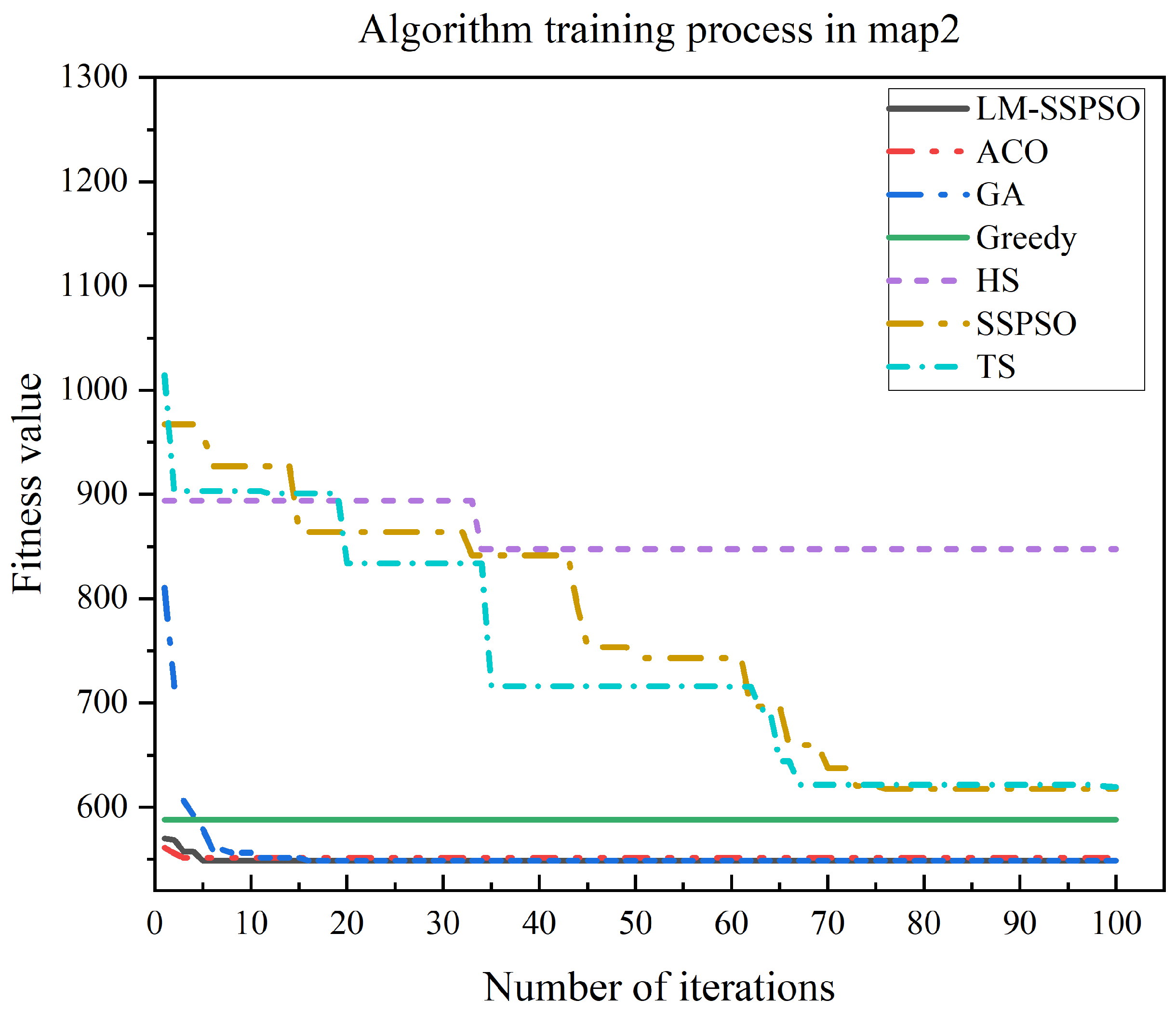As shown in Table 10, the total distance is 560.87, where LM-SSPSO, GA, SSPSO, ACO, and TS can find the shortest path for the multiple goal positions and the 50 calculations. Compared with other algorithms, the LM-SSPSO shows better performance for 50 runs. The maximum value of the LM-SSPSO algorithm is also the smallest. The path planning results of the proposed algorithm and the training process are shown as Figure 10.

4.5. Postprocess of the Optimized Path

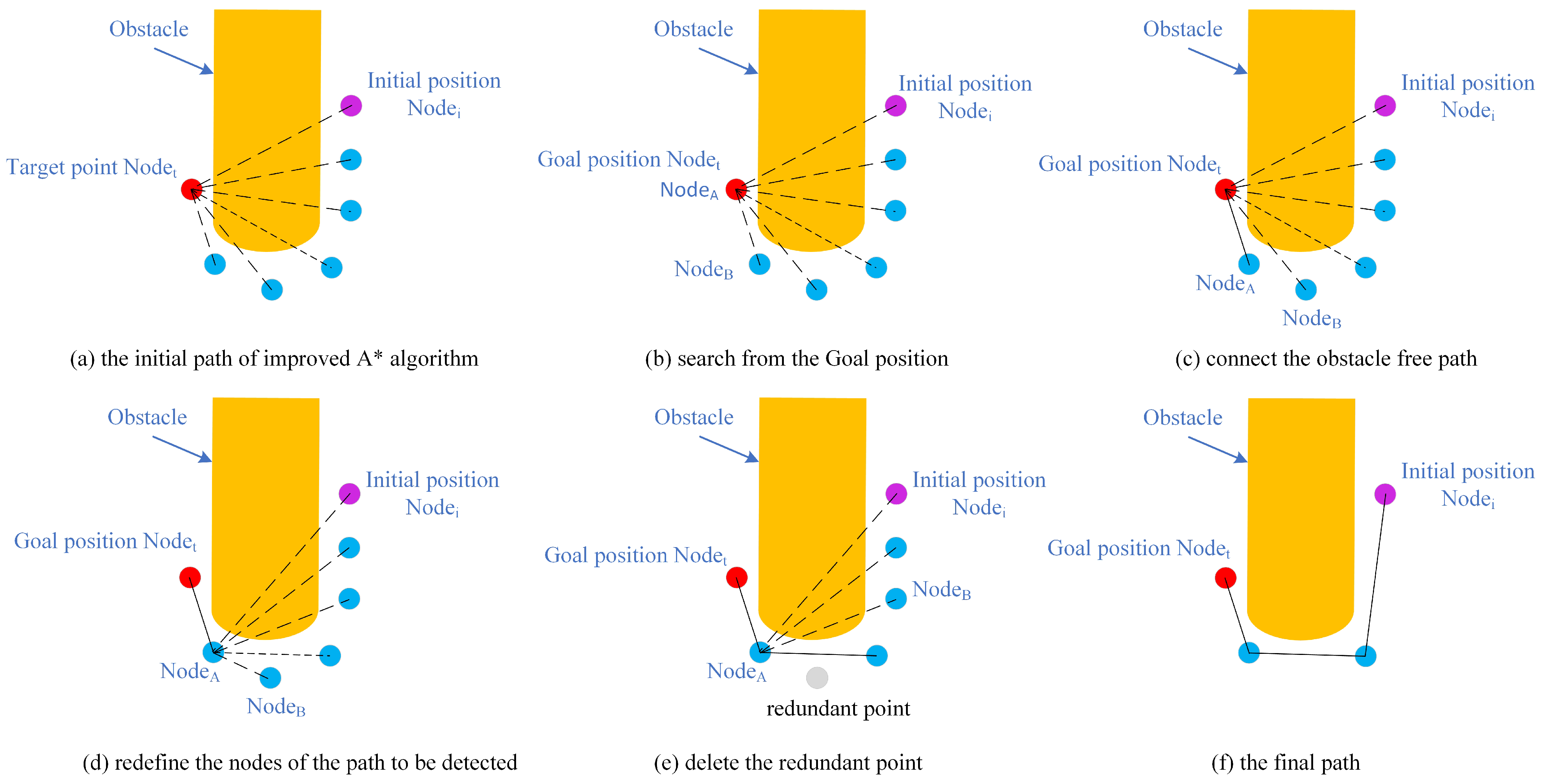
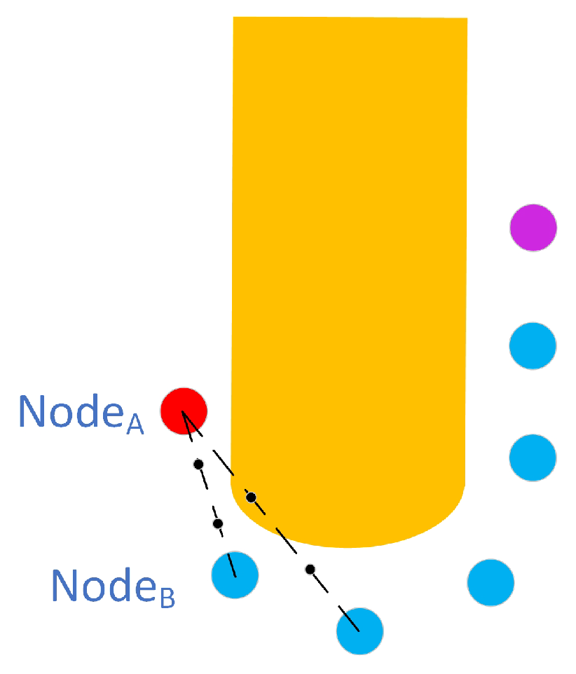
When planning the path, the search area is limited to the local adjacent nodes. As a result, the optimal path may not be obtained. Simultaneously, the variable goal positions in the bidirection can reduce the calculation time; however, the final path may also introduce new redundancy positions, and the efficiency of the robot movement may reduce as a result. To solve this problem, we optimize the path by introducing a postprocessing stage. In Figure 11, the yellow area represents the obstacle, the purple dot $Nod{e}_i$ represents the initial node, the red dot $Nod{e}_t$ is the goal node, and the blue dots are the waypoints. Due to the number of waypoints being significantly higher than usual, as shown in Figure 4, the proposed judgment formulas are unsuitable for the complicated postprocess, and we use sample points to complete the obstacle avoidance task. The postprocessing is described as follows:

Step 1: Initialization. Initialize the obstacle, initial position, waypoint, and goal position.

Step 2: Delete the redundancy point and optimize the path. As shown in Figure 11b, we assign the GOAL node as $Nod{e}_A$ and the adjacent point as $Nod{e}_B$. Connect $Nod{e}_A$ and $Nod{e}_B$, and obtain a dotted line. We divide the dotted line into $N_{dot}$ (for example, $N_{dot}$ = 3) equal parts (Figure 12), and judge whether the divided points (black point) are in the obstacle area or not. If not, we select the next point as $Nod{e}_B$, connect $Nod{e}_A$ and $Nod{e}_B$ to form a new dotted line, and obtain the new divided points. Next, we judge whether the new divided points are in the obstacle or not; if so, as shown in Figure 11d, we connect $Nod{e}_A$ with the previous point of $Nod{e}_B$ using a solid line and delete the redundancy points, as shown in Figure 11e.

Step 3: Optimize the remaining path and obtain the final optimized path. We define the previous point of $Nod{e}_B$ in Step 2 as $Nod{e}_A$. We repeatedly analyze the dotted line between $Nod{e}_A$ and $Nod{e}_B$ as Step 2, and delete the redundancy points until the initial point is $Nod{e}_B$ and its previous point is $Nod{e}_A$. The final optimized path is shown in Figure 11f.

The postprocess results are presented in Figure 13.

5. The Analysis of Improved A* Algorithm and LM-SSPSO PSO in Different Environment Maps

To further verify the effectiveness of the proposed path planning approach, in this section, we compare it with existing approaches in three different environment maps. The environment maps show various obstacles (suspicious positions) and different goal position distributions. The information is presented in Figure 14.

The initial position and all of the goal position coordinate information is shown in

Table 11. The coordinate information of new environment maps.

	1 (Initial Position)	2	3	4	5	6	7	8
Map1	(165, 123)	(144, 108)	(117, 108)	(99, 123)	(78, 87)	(99, 60)	(72, 36)	(54, 63)
Map2	(108, 24)	(27, 15)	(21, 51)	(54, 21)	(27, 78)	(18, 102)	(48, 96)	(36, 123)
Map3	(162, 15)	(81, 39)	(126, 30)	(45, 12)	(63, 48)	(42, 60)	(72, 63)	(33, 105)
	9	10	11	12	13	14	15	16
Map1	(156, 63)	(123, 30)	(54, 102)	(75, 123)	(90,150)	(105, 159)	(123, 165)	(114, 150)
Map2	(54, 144)	(18, 144)	(102, 129)	(126, 96)	(162, 120)	(150, 45)	(156, 75)	(120, 63)
Map3	(51, 123)	(81, 162)	(108, 123)	(153, 129)	(81, 135)	(96, 90)	(141, 72)	(138, 54)

.

5.1. Comparison Analysis of the Computation Time between Any Two Positions at Different Resolutions

All the parameters were set as shown in Table 9. The comparison results of the improved A* algorithms proposed in this paper using traditional A* for the computational time are given.

From

Table 12. The average computation time comparing the results on map1 at different resolutions.

Resolution	Traditional A* Algorithm(s)	Bidirectional Dynamic OpenList Cost Weight A* Algorithm(s)
$120\times 120$	56.24	43.75
$180\times 180$	127.43	88.02
$240\times 240$	332.38	215.5

,

Table 13. The average computation time comparing the results on map2 at different resolutions.

Resolution	Traditional A* Algorithm(s)	Bidirectional Dynamic OpenList Cost Weight A* Algorithm(s)
$120\times 120$	63.08	14.04
$180\times 180$	197.68	26.98
$240\times 240$	432.47	45.59

,

Table 14. The average computation time comparing the results on map3 at different resolutions.

Resolution	Traditional A* Algorithm(s)	Bidirectional Dynamic OpenList Cost Weight A* Algorithm(s)
$120\times 120$	82.94	14.5
$180\times 180$	208.22	30.58
$240\times 240$	544.19	52.97

and

Table 15. Simulation comparison results of different weight coefficients with average computational time for different environment maps.

Environment Map	w = 1 (s)	w = 1.5 (s)	w = 2 (s)	Bidirectional Dynamic OpenList Cost Weight A* Algorithm (s)	${\mathit{w}}_1$ (s)	${\mathit{w}}_2$ (s)	${\mathit{w}}_3$ (s)	${\mathit{w}}_4$ (s)	${\mathit{w}}_5$ (s)
Map1	110.54	95.07	93.55	88.02	138.27	101.28	172.21	431.03	93.95
Map2	92.37	37.28	30.74	26.98	27.391	57.89	51.93	509.31	29.49
Map3	106.12	33.31	31.19	30.58	137.31	39.26	33.86	535.91	41.61

, we obtained the following results.

(1) In the case of the different environment maps, the calculation time of the bidirectional dynamic OpenList cost weight A* algorithm is always less than that of the traditional A* algorithm. The improved A* algorithm has a shorter runtime and higher route planning efficiency.

(2) The calculation time of the bidirectional dynamic OpenList cost weight A* algorithm increases less when the resolution increases. When the resolution of the environment map changes from $120\times 120$ to $180\times 180$ and $120\times 120$ to $240\times 240$, the calculation time multiples calculated via the traditional A* algorithm in the map1 are 2.27, 5.91, and the proposed weights with the A* algorithm are 2.01 and 4.93. For map2, the calculation times multiples calculated via the traditional A* algorithm are 3.13 and 6.86; the proposed weight with the A* algorithm are 1.92, 3.25. For map3, the calculation times multiples calculated via the traditional A* algorithm are 2.51 and 6.56; the bidirectional dynamic OpenList cost weights with the A* algorithm are 2.11 and 3.65. As shown in Table 15, the proposed A* algorithm performs best in different environment maps and consumes the least time.

(3) The results in Table 12, Table 13 and Table 14 show that our path planning method takes less calculation time, especially when the resolutions increase. It has significant advantages in different environment maps and better performance than traditional A* algorithms.

5.2. The Comparison Analysis of the Shortest Distance between Any Two Positions in Different Environment Maps

For the analysis of improved strategy on the shortest distance between any two positions, we defined the resolution of the environment maps as $180\times 180$; the distance matrix between any two positions of all 16 positions was calculated using the 8 adjacent nodes and the 16 adjacent nodes strategy, separately. The distance between the corresponding two positions was also compared, and the results are shown in

Table 16. The shortest distance between any two positions of the 8-neighborhood and 16-neighborhood strategy for map1.

	Neighbor	1 (Initial Point)	2	3	4	5	6	7	8	9	10	11	12	13	14	15	16
1
2	16	29.312
	8	29.312
3	16	103.942	26
	8	52.21	26
4	16	64	45.796	27.656
	8	64	50.21	28.07
5	16	114.968	101.56	93.318	48.484
	8	124.764	115.178	102.726	51.312
6	16	109.662	57.592	51.312	79.452	36.14
	8	101.802	70.49	59.312	90.484	40.554
7	16	135.458	72.63	74.35	99.108	49.656	27.866
	8	139.738	108.012	96.834	106.28	52.484	35.936
8	16	165.082	107.114	100.56	71.866	22.624	42.828	40.484
	8	175.254	143.942	130.834	85.248	31.108	45.242	40.898
9	16	59.726	46.554	45.936	80.834	82.834	54.828	83.936	98
	8	63.554	48.968	60.146	90.216	104.592	57.242	93.178	100
10	16	98.764	72.28	76.07	109.522	60.49	31.038	48.07	70.42	58.898
	8	116.006	84.694	78.484	112.866	76.974	37.936	52.484	81.662	58.898
11	16	152.668	137.044	70.694	42.968	27.796	49.592	59.21	38	114.63	85.184
	8	204.318	166.968	136.28	53.866	28.21	64.49	72.28	38	143.114	100.91
12	16	86	65.28	48.382	20	32.828	65.382	82.828	59.452	120.77	87.248	31.312
	8	88	77.108	55.968	22	35.242	77.796	87.242	66.694	168.044	114.216	34.898
13	16	83.178	48.076	37.866	24.898	62.554	92.694	107.382	84.35	91.388	132.458	49.108	22.21
	8	85.178	69.388	51.178	29.726	66.968	108.522	119.452	100.904	113.324	174.974	69.522	32.21
14	16	66.35	51.522	47.726	36.07	59.936	108.834	119.904	86.904	92.076	159.802	59.248	33.522	16.484
	8	77.592	66.146	54.968	36.484	81.178	126.178	142.388	115.114	115.114	136.28	83.732	46.42	17.312
15	16	66.108	71.764	60.522	45.452	78.42	103.866	148.012	102.974	110.7	136.312	76.076	47.592	28.554	18.07
	8	82.038	88.522	77.522	51.522	96.216	123.694	170.082	130.152	124.77	138.312	98.77	63.388	38.21	18.484
16	16	50.624	37.866	38.828	22.14	67.866	105.49	122.458	94.834	81.592	116.484	64.35	37.038	22	8.484	16.484
	8	65.866	52.42	41.242	32.21	76.49	107.522	145.872	110.426	103.388	121.726	78.63	49.178	22	11.312	17.312

,

Table 17. The shortest distance between any two positions of 8-neighborhood and 16-neighborhood strategies for map2.

	Neighbor	1 (Initial Point)	2	3	4	5	6	7	8	9	10	11	12	13	14	15	16
1
2	16	84.554
	8	84.554
3	16	121.286	33.968
	8	125.63	39.796
4	16	52.828	25.656	55.522
	8	53.242	28.484	64.35
5	16	93.528	65.796	24.07	68.318
	8	102.356	67.796	28.484	70.318
6	16	113.738	84.484	48.828	99.216	23.726
	8	128.566	90.554	51.242	123.458	26.554
7	16	82.216	98.146	45.936	72.624	22.554	36.866
	8	97.184	111.802	55.178	80.624	29.382	37.28
8	16	113.942	111.42	75.006	96.108	43.35	19.796	26.554
	8	130.152	118.834	82.834	112.592	55.764	27.452	30.968
9	16	135.872	147.146	92.904	119.656	62.694	39.592	44.07	21.796
	8	155.05	158.802	110.63	123.656	82.764	54.904	48.484	27.038
10	16	133.324	124.312	90.828	140.7	62.312	40	43.936	19.796	44.28
	8	157.604	133.382	93.242	167.114	69.382	40	58.42	26.624	48.28
11	16	130.668	135.458	83.942	110.458	73.974	79.866	58.764	63.656	51.796	86.592
	8	151.668	154.426	111.464	137.496	95.114	93.178	65.662	66.484	52.21	98.006
12	16	77.038	103.324	98.834	77.528	98.662	107.592	86.936	82.592	69.388	98.904	38.624
	8	77.452	132.362	123.458	103.808	114.146	117.592	91.936	100.006	89.872	128.216	41.936
13	16	127.496	143.12	144.426	109.324	150.496	142.222	118.286	121.452	102.624	139.866	55.038	62.178
	8	138.98	186.916	189.534	157.604	184.152	195.464	176.566	131.038	115.936	157.592	65.038	59.522
14	16	41.866	120.35	133.694	90.866	122.764	136.49	100.146	113.184	117.98	124.566	96.006	69.904	79.382
	8	48.694	135.248	136.108	107.248	136.49	162.7	121.942	154.362	156.19	183.642	114.974	83.146	79.796
15	16	60.076	129.63	137.216	103.802	125.108	134.044	96.662	120.012	90.012	125.98	56.49	22.624	42.484	26.14
	8	80.974	175.324	171.044	137.044	136.694	169.528	128.458	150.222	128.566	168.566	75.114	36.694	47.312	32.968
16	16	38.898	100.006	95.312	64.56	90.554	104.764	64.764	82.974	87.286	97.598	62.968	28.07	56.834	29.554	39.694
	8	42.968	111.7	102.968	82.388	98.21	131.044	91.286	140.878	115.324	159.464	71.452	34.484	74.974	39.038	47.522

and

Table 18. The shortest distance between any two positions of 8-neighborhood and 16-neighborhood strategies for map3.

	Neighbor	1 (Initial Point)	2	3	4	5	6	7	8	9	10	11	12	13	14	15	16
1
2	16	94.076
	8	94.076
3	16	35.382	45.866
	8	40.21	51.866
4	16	122.624	42.35	87.318
	8	123.866	46.764	102.662
5	16	101.7	16.898	63.108	47.312
	8	119.114	19.726	71.108	47.312
6	16	114.974	41.866	77.936	84.248	24.484
	8	136.63	46.694	94.42	91.726	27.312
7	16	84.388	20.484	51.108	56.624	12.898	28.828
	8	108.872	25.726	65.662	67.038	17.726	29.242
8	16	157.706	85.452	105.77	112.592	73.108	61.834	63.452
	8	184.948	93.662	142.738	127.038	78.694	68.936	69.452
9	16	146.604	82.35	97.566	118.038	66.554	95.146	55.796	30.382
	8	194.158	100.56	151.706	126.624	78.968	100.522	72.866	32.726
10	16	170.286	149.566	156.426	176.254	129.91	134.496	114.012	146.738	117.082
	8	184.292	223.904	153.732	209.7	213.146	155.668	201.006	162.006	143.694
11	16	126.458	92.318	90.968	121.152	74.114	80.7	63.318	72.968	54	50.452
	8	147.566	105.802	101.108	156.846	118.254	96.082	99.318	81.452	56	52.28
12	16	114.484	106.668	99.834	123.808	87.184	117.668	80.56	116.936	102.49	81.592	56.834
	8	115.726	117.808	113.904	166.572	126.98	155.464	113.184	138.35	125.318	85.248	71.42
13	16	126.77	103.248	101.216	131.49	84.662	68.006	65.248	43.866	27.312	132.948	27.312	76.42
	8	158.502	122.936	122.63	144.248	107.662	90.146	94.178	58.42	32.968	145.484	30.968	84.834
14	16	83.802	45.592	55.108	85.458	45.248	56.732	43.866	63.038	46.28	75.452	32.14	61.42	42.554
	8	102.98	64.49	70.42	111.254	74.076	85.872	57.866	71.522	57.662	85.452	36.968	79.732	50.21
15	16	61.796	69.63	42.694	100.082	68.216	96.426	64.592	104.076	88.7	99.248	49.522	53.726	63.388	46.624
	8	65.866	84.942	54.592	130.534	97.63	140.496	83.42	130.044	117.426	117.942	63.662	60.968	86.426	54.694
16	16	42.624	53.382	21.312	110.77	71.484	91.522	58.108	124.49	116.044	115.91	59.974	72.14	86.012	45.006	20.968
	8	47.936	62.21	26.968	115.184	77.14	106.178	75.28	149.942	157.324	144.464	92.942	80.21	115.464	65.802	28.796

, where bold font represents the better solution with small fitness.

The simulations results of

Table 19. The comparison of the results of 8 adjacent nodes and 16 adjacent nodes path lengths.

	16 Adjacent Nodes Path Length Is Shorter	Path Lengths Are Equal	8 Adjacent Nodes Path Length Is Shorter
Number(map1)	111	6	3
Number(map2)	117	2	1
Number(map3)	117	2	1

were used to analyze the effect of node numbers on the performance of the shortest distance path. The results show that the 16 adjacent nodes strategy provided better performance than the 8 adjacent nodes method. The 16 adjacent nodes strategy is stable and effective when it comes to finding the shortest path between any two positions in different maps. To obtain a shorter distance path, the shorter distance between any two positions generated by using 16 adjacent nodes, and 8 adjacent nodes are selected to form a new distance matrix (

Table 20. The shortest distance between any two positions of map1.

	1 (Initial Position)	2	3	4	5	6	7	8	9	10	11	12	13	14	15	16
1	0	29.312	52.21	64	114.968	101.802	135.458	165.082	59.726	98.764	152.668	86	83.178	66.35	66.108	50.624
2	29.312	0	26	45.796	101.56	57.592	72.63	107.114	46.554	72.28	137.044	65.28	48.076	51.522	71.764	37.866
3	52.21	26	0	27.656	93.318	51.312	74.35	100.56	45.936	76.07	70.694	48.382	37.866	47.726	60.522	38.828
4	64	45.796	27.656	0	48.484	79.452	99.108	71.866	80.834	109.522	42.968	20	24.898	36.07	45.452	22.14
5	114.968	101.56	93.318	48.484	0	36.14	49.656	22.624	82.834	60.49	27.796	32.828	62.554	59.936	78.42	67.866
6	101.802	57.592	51.312	79.452	36.14	0	27.866	42.828	54.828	31.038	49.592	65.382	92.694	108.834	103.866	105.49
7	135.458	72.63	74.35	99.108	49.656	27.866	0	40.484	83.936	48.07	59.21	82.828	107.382	119.904	148.012	122.458
8	165.082	107.114	100.56	71.866	22.624	42.828	40.484	0	98	70.42	38	59.452	84.35	86.904	102.974	94.834
9	59.726	46.554	45.936	80.834	82.834	54.828	83.936	98	0	58.898	114.63	120.77	91.388	92.076	110.7	81.592
10	98.764	72.28	76.07	109.522	60.49	31.038	48.07	70.42	58.898	0	85.184	87.248	132.458	136.28	136.312	116.484
11	152.668	137.044	70.694	42.968	27.796	49.592	59.21	38	114.63	85.184	0	31.312	49.108	59.248	76.076	64.35
12	86	65.28	48.382	20	32.828	65.382	82.828	59.452	120.77	87.248	31.312	0	22.21	33.522	47.592	37.038
13	83.178	48.076	37.866	24.898	62.554	92.694	107.382	84.35	91.388	132.458	49.108	22.21	0	16.484	28.554	22
14	66.35	51.522	47.726	36.07	59.936	108.834	119.904	86.904	92.076	136.28	59.248	33.522	16.484	0	18.07	8.484
15	66.108	71.764	60.522	45.452	78.42	103.866	148.012	102.974	110.7	136.312	76.076	47.592	28.554	18.07	0	16.484
16	50.624	37.866	38.828	22.14	67.866	105.49	122.458	94.834	81.592	116.484	64.35	37.038	22	8.484	16.484	0

,

Table 21. The shortest distance between any two positions of map2.

	1 (Initial Position)	2	3	4	5	6	7	8	9	10	11	12	13	14	15	16
1	0	84.554	121.286	52.828	93.528	113.738	82.216	113.942	135.872	133.324	130.668	77.038	127.496	41.866	60.076	38.898
2	84.554	0	33.968	25.656	65.796	84.484	98.146	111.42	147.146	124.312	135.458	103.324	143.12	120.35	129.63	100.006
3	121.286	33.968	0	55.522	24.07	48.828	45.936	75.006	92.904	90.828	83.942	98.834	144.426	133.694	137.216	95.312
4	52.828	25.656	55.522	0	68.318	99.216	72.624	96.108	119.656	140.7	110.458	77.528	109.324	90.866	103.802	64.56
5	93.528	65.796	24.07	68.318	0	23.726	22.554	43.35	62.694	62.312	73.974	98.662	150.496	122.764	125.108	90.554
6	113.738	84.484	48.828	99.216	23.726	0	36.866	19.796	39.592	40	79.866	107.592	142.222	136.49	134.044	104.764
7	82.216	98.146	45.936	72.624	22.554	36.866	0	26.554	44.07	43.936	58.764	86.936	118.286	100.146	96.662	64.764
8	113.942	111.42	75.006	96.108	43.35	19.796	26.554	0	21.796	19.796	63.656	82.592	121.452	113.184	120.012	82.974
9	135.872	147.146	92.904	119.656	62.694	39.592	44.07	21.796	0	44.28	51.796	69.388	102.624	117.98	90.012	87.286
10	133.324	124.312	90.828	140.7	62.312	40	43.936	19.796	44.28	0	86.592	98.904	139.866	124.566	125.98	97.598
11	130.668	135.458	83.942	110.458	73.974	79.866	58.764	63.656	51.796	86.592	0	38.624	55.038	96.006	56.49	62.968
12	77.038	103.324	98.834	77.528	98.662	107.592	86.936	82.592	69.388	98.904	38.624	0	59.522	69.904	22.624	28.07
13	127.496	143.12	144.426	109.324	150.496	142.222	118.286	121.452	102.624	139.866	55.038	59.522	0	79.382	42.484	56.834
14	41.866	120.35	133.694	90.866	122.764	136.49	100.146	113.184	117.98	124.566	96.006	69.904	79.382	0	26.14	29.554
15	60.076	129.63	137.216	103.802	125.108	134.044	96.662	120.012	90.012	125.98	56.49	22.624	42.484	26.14	0	39.694
16	38.898	100.006	95.312	64.56	90.554	104.764	64.764	82.974	87.286	97.598	62.968	28.07	56.834	29.554	39.694	0

and

Table 22. The shortest distance between any two positions of map3.

	1 (Initial Position)	2	3	4	5	6	7	8	9	10	11	12	13	14	15	16
1	0	94.076	35.382	122.624	101.7	114.974	84.388	157.706	146.604	170.286	126.458	114.484	126.77	83.802	61.796	42.624
2	94.076	0	45.866	42.35	16.898	41.866	20.484	85.452	82.35	149.566	92.318	106.668	103.248	45.592	69.63	53.382
3	35.382	45.866	0	87.318	63.108	77.936	51.108	105.77	97.566	153.732	90.968	99.834	101.216	55.108	42.694	21.312
4	122.624	42.35	87.318	0	47.312	84.248	56.624	112.592	118.038	176.254	121.152	123.808	131.49	85.458	100.082	110.77
5	101.7	16.898	63.108	47.312	0	24.484	12.898	73.108	66.554	129.91	74.114	87.184	84.662	45.248	68.216	71.484
6	114.974	41.866	77.936	84.248	24.484	0	28.828	61.834	95.146	134.496	80.7	117.668	68.006	56.732	96.426	91.522
7	84.388	20.484	51.108	56.624	12.898	28.828	0	63.452	55.796	114.012	63.318	80.56	65.248	43.866	64.592	58.108
8	157.706	85.452	105.77	112.592	73.108	61.834	63.452	0	30.382	146.738	72.968	116.936	43.866	63.038	104.076	124.49
9	146.604	82.35	97.566	118.038	66.554	95.146	55.796	30.382	0	117.082	54	102.49	27.312	46.28	88.7	116.044
10	170.286	149.566	153.732	176.254	129.91	134.496	114.012	146.738	117.082	0	50.452	81.592	132.948	75.452	99.248	115.91
11	126.458	92.318	90.968	121.152	74.114	80.7	63.318	72.968	54	50.452	0	56.834	27.312	32.14	49.522	59.974
12	114.484	106.668	99.834	123.808	87.184	117.668	80.56	116.936	102.49	81.592	56.834	0	76.42	61.42	53.726	72.14
13	126.77	103.248	101.216	131.49	84.662	68.006	65.248	43.866	27.312	132.948	27.312	76.42	0	42.554	63.388	86.012
14	83.802	45.592	55.108	85.458	45.248	56.732	43.866	63.038	46.28	75.452	32.14	61.42	42.554	0	46.624	45.006
15	61.796	69.63	42.694	100.082	68.216	96.426	64.592	104.076	88.7	99.248	49.522	53.726	63.388	46.624	0	20.968
16	42.624	53.382	21.312	110.77	71.484	91.522	58.108	124.49	116.044	115.91	59.974	72.14	86.012	45.006	20.968	0

) for the following optimization process.

5.3. Performance Analysis of LM-SSPSO with Other Approaches for Traversing All Goal Positions for Different Environment Maps

In

Table 23. Numbers of obtained optimal solutions using different algorithms.

	map1	map2	map3
LM-SSPSO	50	50	50
HS	0	0	0
SSPSO	1	2	1
Greedy	0	0	0
GA	26	50	13
ACO	1	32	0
TS	2	10	2

,

Table 24. The maximum value of all 50 loops using different algorithms.

	map1	map2	map3
LM-SSPSO	478.1	548.966	656.22
HS	868.672	1131.88	1098.772
SSPSO	660.386	736.952	833.11
Greedy	511.138	588.208	779.168
GA	491.826	548.966	667.022
ACO	491.826	551.246	674.398
TS	612.316	750.812	788.27

,

Table 25. The average value of all 50 loops using different algorithms.

	map1	map2	map3
LM-SSPSO	478.1	548.966	656.22
HS	814.49	998.6336	1018.1468
SSPSO	550.2192	633.4848	723.9666
Greedy	511.138	588.208	779.168
GA	481.634	548.966	664.27
ACO	481.0868	549.3308	667.97
TS	523.8512	600.8568	692.771

and

Table 26. The minimum value of all 50 loops using different algorithms.

	map1	map2	map3
LM-SSPSO	478.1	548.966	656.22
HS	715.59	845.812	856.722
SSPSO	478.1	548.966	656.022
Greedy	511.138	548.966	779.168
GA	478.1	548.966	656.22
ACO	478.1	548.966	666.5
TS	478.1	548.966	656.22

and Figure 15, Figure 16 and Figure 17, the parameter settings are the same as in Table 9. The numbers of the optimal solution obtained by using different algorithms are shown as below.

As shown in Table 23, SSPSO, GA, TS, and LM-SSPSO successfully found the optimal path for all three environment maps. Compared with the other intelligent algorithms, the LM-SSPSO showed better performance and a higher probability of obtaining the optimal path in the different maps.

The optimal paths of map1, map2, and map3 are $1\to 2\to 3\to 4\to 16\to 15\to 14\to 13\to 12\to 11\to 5\to 8\to 7\to 6\to 10\to 9\to 1;$ $1\to 14\to 16\to 12\to 15\to 13\to 11\to 9\to 8\to 10\to 6\to 7\to 5\to 3\to 2\to 4\to 1;$ $1\to 3\to 2\to 4\to 5\to 7\to 6\to 8\to 9\to 13\to 14\to 11\to 10\to 12\to 15\to 16\to 1$, and the shortest distances are 478.1, 548.966, and 656.22, respectively. The convergence speed of the algorithm is fast and the optimal solution calculated for the first time for map1, map2, and map3 are 5, 5, and 12, respectively.

According to Table 24, Table 25 and Table 26, we can observe that the LM-SSPSO is much more effective in terms of calculating the minimum value, maximum value, and average value than other algorithms for the different maps. The convergence speed of particles was significantly improved, as shown in Figure 15, Figure 16 and Figure 17. It is clear that the solutions calculated using LM-SSPSO were always better than those that were calculated using other algorithms given its characteristics with the optimal initial solution, avoiding the local optimum and optimal selection.

The path generated by the proposed algorithm with postprocessing is shown in Figure 18.

6. Conclusions

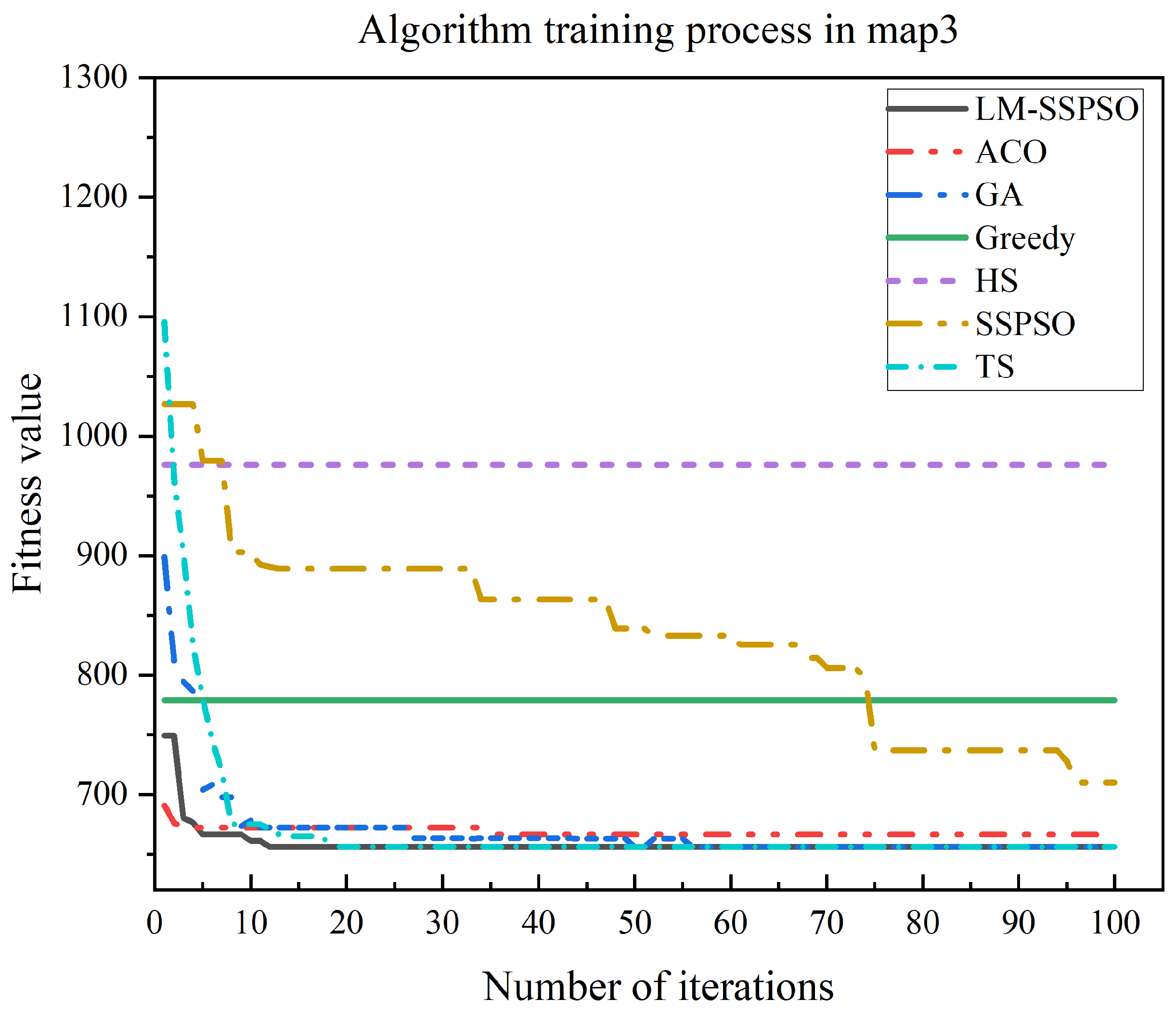
In this paper, we introduced a novel approach to multiple-goal position path planning. Two problems were solved. The first problem involved finding the shortest distance between any two positions, and the other involved finding the shortest distance path which traverses all the goal positions. When solving the first problem, we introduced a bidirectional strategy and dynamic OpenList cost weight strategy into the A* algorithm. As the resolution of the first environment map changed from $120\times 120$ to $180\times 180$ and $120\times 120$ to $240\times 240$, the calculation time was less than that of traditional A* algorithm. The obtain time multiples were 1.90 and 3.16, respectively. These are significantly less than those of the traditional A* algorithm. When comparing with different weight coefficients, the proposed algorithm required the shortest time with 50.27 s at $180\times 180$ resolution. Based on the proposed time optimization strategy, we also extended the search nodes from 8 to 16 adjacent nodes and introduced a new obstacle judgment formula to analyze the obstacles. Compared with the distance in the 8 adjacent nodes’ distance matrix, 115 path length in 16 adjacent nodes was shorter; the others were equal to 8 adjacent nodes. Compared with the GORRT algorithm, in 16 adjacent nodes, 119 path lengths were shorter, and 1 was longer. When tackling the second problem, we developed the LM-SSPSO strategy to purposefully optimize all the processes of PSO. First, the initial solutions are optimized by using the greedy algorithm, association strategy, and analysis strategy to obtain the local optimal solutions. Then, the comparison, forgetting–reinforcement, and diverse thinking strategy are used to maintain diversity, accelerating particles convergence. The swap sequence strategy is also used in the process of forgetting–reinforcement, and a forget probability function and a reinforcement probability function are used to avoid a local optimum. Finally, the retention idea was also introduced to obtain a better swarm. Compared with six other intelligent algorithms, the LM-SSPSO showed the best performance with the shortest Minmum, Maximum, Average path length 560.87 in the 50 loop computations. It also obtained a higher success rate in finding the optimal solution. After obtaining the multiple-goal-positions path, the redundant points are also removed in the postprocessing. Additionally, the results of comparative experiments were analyzed using three new environment maps. The simulation results further verified that the proposed algorithm’s performance is efficient across different environment maps.

In future work, we will improve our proposed BD-A* algorithm with novel criteria to reduce searching nodes and add a guide line to accelerate the search process and optimize the calculation time. We will optimize the swarm size of LM-SSPSO and analyze the influence of different strategies on the performance of LM-SSPSO, so that we can improve the effectiveness of the LM-SSPSO algorithm. Additionally, we will also focus our research on multiobjective function optimization, which includes torque, global energy reductions, shortest distance, etc. A dynamic environment will also be considered. We may apply our path planning method with the Pareto set strategy and create a real-time application of multiple-goal positions path planning in a dynamic environment.