Evaluation of Hamiltonians from Complex Symplectic Matrices

Abstract

Gaussian unitaries play a fundamental role in the field of continuous variables. In the general n mode, they may formulated by a second-order polynomial in the bosonic operators. Another important role related to Gaussian unitaries is played by the symplectic transformations in the phase space. The paper investigates the links between the two representations: the link from Hamiltonian to symplectic, governed by an exponential, and the link from symplectic to Hamiltonian, governed by a logarithm. Thus, an answer is given to the non-trivial question: which Hamiltonian produces a given symplectic representation? The complex instead of the traditional real symplectic representation is considered, with the advantage of getting compact and elegant relations. The application to the single, two, and three modes illustrates the theory.

1. Introduction

In the last three decades, continuous variable systems have been the object of great attention for the development of quantum information, transmission, and processing. Thence, a great deal of theoretical work on Gaussian states and transformation for both single-mode and multimode systems has been carried out [1,2,3,4].

The paper deals with Gaussian unitaries, starting from the definition, which in turn is based on the definition of a Gaussian state. In the general n mode, a quantum state (pure or mixed) is said to be Gaussian if its Wigner function is given by a $2n$ multivariate Gaussian function [4,5]. Therefore, the definition of a Gaussian unitary is very simple: “a Gaussian unitary is a unitary transformation that preserves Gaussian states” [6].

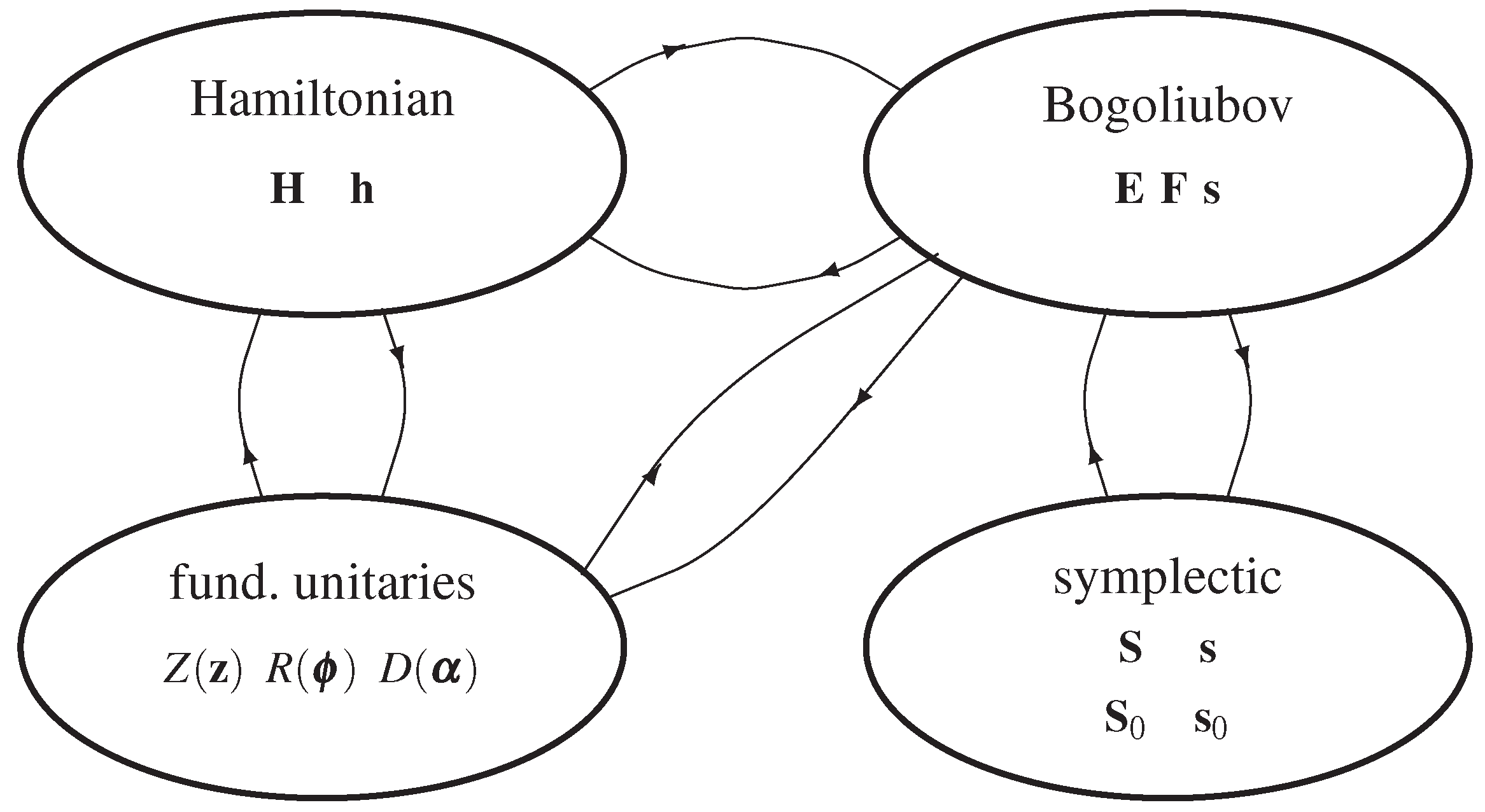
Now, there are several “specifications” of Gaussian unitaries, that is, several ways to formalize the information needed to identify a Gaussian unitary. We concentrate our attention on four “specifications”:

1.

Hamiltonian specification, given by a second-order polynomial in the bosonic operators;

2.

Bogoliubov specification, based on Bogoliubov transformations;

3.

FGU specification in the Hilbert space (FGU = fundamental Gaussian unitary);

4.

Symplectic specification in the phase space.

These specifications are equivalent in the representation of the whole class of Gaussian unitaries in the sense that it is possible to obtain any specification from the others [7], as shown in Figure 1.

The purpose of the paper is the formulation of the links between the different representations, as illustrated in Figure 1. The link $(\mathbf{H},\mathbf{h})\to (\mathbf{S},\mathbf{s})$ is known in the literature (see, e.g., the paper by Adesso, Ragy, and Lee [8]), but the formulation of the inverse link $(\mathbf{S},\mathbf{s})\to (\mathbf{H},\mathbf{h})$ seems to be new. The latter gives an answer to the question: which Hamiltonian is needed to produce a given symplectic transformation or a given Bogoliubov transformation?

The paper is organized as follows. In Section 2, we introduce the matrix representations. In Section 3, we introduce the matrix representation $(\mathbf{H},\mathbf{h})$ of quadratic Hamiltonians. In Section 4, we develop the path “Hamiltonian → symplectic representation”. Both representations may be regarded as an algebraic specification. But in Section 5, we also express the two representations in terms of the so-called fundamental Gaussian unitaries (FGUs): displacement, rotation, and squeezing, according to the theory of Ma and Rhodes of 1990 [9] (see also [10]). This allows us to obtain a physical insight on the operations involved. In Section 6, we develop the path symplectic-to-Hamiltonian representation. Note that, while the direct path is formulated in term of an exponential, essentially the exponential of a square matrix, the inverse path involves the logarithm of a square matrix, with delicate problems of uniqueness, as discussed in an important book by Higham [11]. In Section 7 and Section 8, we apply the theory to single, two, and three modes. In the Appendix A we outline an overview of the functions of complex matrices, in particular of the logarithm.

2. Formulation of Specifications

In this section, we introduce the specifications, mainly the matrix reprentations.

The Hamiltonian specification is supported by a fundamental theorem [9,12], which states that a unitary operator $U=e^{-iH}$, where the Hamiltonian H is a second-order polynomial (briefly: quadratic) in the bosonic operators $a_i^{\ast }$ and $a_i$, is a Gaussian unitary. Then, H can be handled using a matrix representation $(\mathbf{H},\mathbf{h})$, having the structure

$$\mathbf{H}=\left[\begin{array}{cc}\mathbf{A}& \mathbf{B}\\ \overline{\mathbf{B}}& \overline{\mathbf{A}}\end{array}\right],\mathbf{h}=\left[\begin{array}{c}{\mathbf{h}}_1\\ {\overline{\mathbf{h}}}_1\end{array}\right]$$

(1)

where in the n mode, $\mathbf{H}$ is a $2n\times 2n$ complex matrix and $\mathbf{h}$ is a $2n$ complex vector. From Hamiltonians, one can derive complex symplectic transformations $\xi \to \mathbf{S}\xi +\mathbf{s}$, where $\xi$ collects all the $2n$ bosonic operators $\mathbf{a},{\mathbf{a}}_{\ast }$, $\mathbf{S}$ is a $2n\times 2n$ matrix, and $\mathbf{s}$ is a 2n complex vector with the same block structure and dimension as H and $\mathbf{h}$, namely

$$\mathbf{S}=\left[\begin{array}{cc}\mathbf{E}& \mathbf{F}\\ \overline{\mathbf{F}}& \overline{\mathbf{E}}\end{array}\right],\mathbf{s}=\left[\begin{array}{c}{\mathbf{s}}_1\\ {\overline{\mathbf{s}}}_1\end{array}\right].$$

(2)

The representation (1) is developed in [8] and, although achieved with a trivial recast of symbols, has several advantages with respect to the traditional Bogoliubov form, namely: (1) $\mathbf{S}$ is directly given by an exponential of $\mathbf{H}$ as $\mathbf{S}=exp(-i\mathrm{\Omega }\mathbf{H})$, (2) $\mathbf{S}$ generates directly the Bogoliubov matrices $\mathbf{E}$ and $\mathbf{F}$, as indicated in (2), and (3) $\mathbf{S}$ is simply related to the traditional real symplectic matrix ${\mathbf{S}}_0$ of the phase space. In other words, the compact form (2) provides both the Bogoliubov transformation and the passage to the phase space. For these reasons, we call $\mathbf{S}$complex symplectic matrix and the compact form $\xi \to \mathbf{S}\xi +\mathbf{s}$ complex symplectic transformation.

Note that the global parameters $(\mathbf{H},\mathbf{h})$ and $(\mathbf{S},\mathbf{s})$ are redundant, as clear from (1) and (2), while the essential parameters $(\mathbf{A},\mathbf{B},{\mathbf{h}}_1)$ and $(\mathbf{E},\mathbf{F},{\mathbf{s}}_1)$ contain the information of the global parameters in a minimal form.

Normalization. We consider n-mode quantum states and denote by $a_k$ and $a_k^{\ast }$ the bosonic operators of the k mode and by $q_k$ and $p_k$ the quadrature operators, given by $q_k=(a_k+a_k^{\ast })/\sqrt{2}$, $p_k=-i(a_k-a_k^{\ast })/\sqrt{2}$. The commutation conditions are $[a_k,a_{\ell }^{\ast }]={\delta }_{kl}$,$[a_k,a_{\ell }]=0$ and $[q_k,p_k]=i$, $[q_k,q_{\ell }]=[p_k,q_{\ell }]=0$, $\ell \ne k$.

A brief story. Hamiltonian mechanics emerged in 1833 as a reformulation of Lagrangian mechanics, and were introduced by Sir William Rowan Hamilton [13,14]. The term “symplectic” was introduced in 1939 by Hermann Weyl in the context of symplectic geometry, a branch of differential geometry and differential topology that studies differentiable manifolds [15,16]. The Bogoliubov transformations were formulated by Nikolay Nikolayevich Bogolyubov in 1958 in the context of the theory of superconductivity [17]. The fundamental Gaussian unitaries were formulated by Xin Ma and William Rhodes in the generalization of squeezed states [9].

A preliminary definition. A $2n\times 2n$ Hermitian matrix with the redundant structure

$$\mathbf{W}=\left[\begin{array}{cc}\mathbf{X}& \mathbf{Y}\\ \overline{\mathbf{Y}}& \overline{\mathbf{X}}\end{array}\right]$$

(3)

is called complex symplectic if it verifies the symplectic condition

$$\mathbf{W}\mathrm{\Omega }{\mathbf{W}}^{\ast }=\mathrm{\Omega }\mathrm{with}\mathrm{\Omega }=\left[\begin{array}{cc}\mathbf{I}& \mathbf{0}\\ \mathbf{0}& -\mathbf{I}\end{array}\right]$$

(4)

($\mathbf{I}$ is the $n\times n$ identity matrix). Note that condition (4) at block level becomes

$$\mathbf{X}{\mathbf{X}}^{\ast }-\mathbf{Y}{\mathbf{Y}}^{\ast }=\mathbf{I},\mathbf{X}{\mathbf{Y}}^{\mathrm{T}}={\left(\mathbf{X}{\mathbf{Y}}^{\mathrm{T}}\right)}^{\mathrm{T}}$$

(5)

and the Hermiticity is ensured by the conditions

$${\mathbf{X}}^{\ast }=\mathbf{X},{\mathbf{Y}}^{\mathrm{T}}=\mathbf{Y}$$

(6)

3. Quadratic Hamiltonians

A Gaussian unitary is defined as a unitary operator that transforms a Gaussian state into a Gaussian state. From this definition, one can prove that (see Section IV of the paper by Ma and Rhodes [5,9]) a unitary operator $U=e^{-iH}$, where the Hamiltonian H is quadratic polynomial in the bosonic operators $a_m^{\ast }$ and $a_m$, is a Gaussian unitary.

Matrix Representation of a Quadratic Hamiltonian

In the n bosonic mode, a quadratic Hamiltonian has the form below. (The linear term is omitted by several authors, e.g., in [8], because it can be absorbed by local displacements.)

$$H=\frac{1}{2}\sum _{r,s=1}^n\left[A_{rs}{a}_r^{\ast }{a}_s+{\overline{A}}_{rs}{a}_r{a}_s^{\ast }\right]+\frac{1}{2}\sum _{r,s=1}^n\left[B_{rs}{a}_r^{\ast }{a}_s+{\overline{B}}_{rs}{a}_r{a}_s^{\ast }\right]+\sum _{r=1}^n\left(h_r{a}_r^{\ast }+{\overline{h}}_r{a}_r\right)$$

(7)

where the bar denotes the complex conjugate. Collecting the coefficients $A_{rs}$, $B_{rs}$, and $h_r$ in the matrices $\mathbf{A}$, $\mathbf{B}$, and in the column vector $\mathbf{h}$, the Hamiltonian takes the compact form

$$H=\frac{1}{2}{\xi }^{\ast }\mathbf{H}\xi +{\mathbf{h}}^{\mathrm{T}}\xi$$

(8)

where

$$\xi :=\left[\begin{array}{c}\mathbf{a}\\ {\mathbf{a}}_{\ast }\end{array}\right]\mathrm{with}\mathbf{a}:=\left[\begin{array}{c}{a}_1\\ ⋮\\ a_n\end{array}\right],{\mathbf{a}}_{\ast }:=\left[\begin{array}{c}{a}_1^{\ast }\\ ⋮\\ a_n^{\ast }\end{array}\right],$$

(9)

and

$$\mathbf{H}=\left[\begin{array}{cc}\mathbf{A}& \mathbf{B}\\ \overline{\mathbf{B}}& \overline{\mathbf{A}}\end{array}\right],\mathbf{h}=\left[\begin{array}{c}{\mathbf{h}}_1\\ \overline{{\mathbf{h}}_1}\end{array}\right]\mathrm{with}{\mathbf{h}}_1=\left[\begin{array}{c}{h}_1\\ ⋮\\ h_n\end{array}\right]$$

(10)

$\mathbf{H}$ is a $2n\times 2n$ Hermitian matrix and $\mathbf{h}$ is a $2n$ complex column vector. The pair $(\mathbf{H},\mathbf{h})$ gives the matrix representation of H. The Hermitian nature of the Hamiltonian implies the conditions

$$\mathbf{A}={\mathbf{A}}^{\ast },\mathbf{B}={\mathbf{B}}^{\mathrm{T}}$$

(11)

that is, $\mathbf{A}$ is Hermitian and $\mathbf{B}$ is symmetric. Then, $\mathbf{H}$ is a $2n\times 2n$ Hermitian matrix.

Parameter budget. The essential parameters of a Hamiltonian are given by the triplet $(\mathbf{A},\mathbf{B},{\mathbf{h}}_1)$, which consists of (1) one $n\times n$ Hermitian matrix, (2) one $n\times n$ symmetric matrix, and (3) one n size complex vector. In terms of real variables, we have: (1) $n^2$ real variables, (2) $n^2+n$ real variables, and (3) $2n$ real variables. Hence, the specification of a general n-mode Hamiltonian in the n mode is given by

$$2n^2+3n\mathrm{real}\mathrm{variables}.$$

(12)

4. Symplectic Transformations from Hamiltonians

Hamiltonians are concerned with the structure of Gaussian unitary operators. A new equivalent specification is obtained by the application of a Gaussian unitary operator to the field operators, which is expressed by a symplectic transformation.

Generation of Symplectic Transformations

The transformation performed by a Gaussian unitary $U=e^{-iH}$, with H a quadratic Hamiltonian, takes an arbitrary linear combination of field operators to another arbitrary linear combination of field operators (symplectic transformation).

Theorem 1. 

The application of the $2n$ field vector $\xi ={[\mathbf{a},{\mathbf{a}}_{\ast }]}^{\mathrm{T}}$ to a Gaussian unitary $U=e^{-iH}$, where H is a quadratic Hamiltonian, provides the transformation

$$e^{iH}\xi e^{-iH}=\mathbf{S}\xi +\mathbf{s}$$

(13)

where

$$\mathbf{S}=e^{-i\mathrm{\Omega }\mathbf{H}},\mathbf{s}=i\mathrm{\Omega }\mathbf{h}\mathrm{with}\mathrm{\Omega }=\left[\begin{array}{cc}\mathbf{I}& \mathbf{0}\\ \mathbf{0}& -\mathbf{I}\end{array}\right]$$

(14)

with $(\mathbf{H},\mathbf{h})$ the matrix representation of H, $\mathbf{S}$ is a $2n\times 2n$ matrix, called the complex symplectic matrix, and $\mathbf{s}$ is a $2n$ complex vector. The matrix $\mathbf{S}$ verifies the symplectic condition

$$\mathbf{S}\mathrm{\Omega }{\mathbf{S}}^{\ast }=\mathrm{\Omega }$$

(15)

which is the symplectic counterpart of conditions (11) on the matrix $\mathbf{H}$.

Theorem 1 may be viewed as the unified version of Bogoliubov transformations, where the use of the Hadamard lemma [18,19] is applied to the general case, whereas in other references, it is usually applied to specific Gaussian unitaries. For proof, see the paper by Adesso, Ragy, and Lee [8]. These authors give the following comment to the above result: “given a unitary operator that can be written as a single exponential, also the corresponding symplectic matrix can be written as a single exponential”.

If we partition $\mathbf{S}$ and $\mathbf{s}$ into blocks

$$\mathbf{S}=\left[\begin{array}{cc}\mathbf{E}& \mathbf{F}\\ \overline{\mathbf{F}}& \overline{\mathbf{E}}\end{array}\right],\mathbf{s}=\left[\begin{array}{c}{\mathbf{s}}_1\\ {\overline{\mathbf{s}}}_1\end{array}\right].$$

(16)

we find that they have the same block structure as $\mathbf{H}$ and $\mathbf{h}$ (this can be proved in the framework of symplectic groups [20]). In particular, in terms of the blocks $\mathbf{E}$ and $\mathbf{F}$, the condition (15) reads

$$\mathbf{E}{\mathbf{E}}^{\ast }-\mathbf{F}{\mathbf{F}}^{\ast }=\mathbf{I},\mathbf{E}{\mathbf{F}}^{\mathrm{T}}={\left(\mathbf{E}{\mathbf{F}}^{\mathrm{T}}\right)}^{\mathrm{T}}.$$

(17)

Usually, symplectic transformations are not expressed in the complex form indicated above. The standard form in the literature is a real symplectic transformation, which is considered below. Here, from Theorem 1, we derive Bogoliubov transformations by partitioning the matrices as in (16). Then, (13) reads

$$e^{iH}\left[\begin{array}{c}\mathbf{a}\\ {\mathbf{a}}_{\ast }\end{array}\right]e^{-iH}=\left[\begin{array}{cc}\mathbf{E}& \mathbf{F}\\ \overline{\mathbf{F}}& \overline{\mathbf{E}}\end{array}\right]\left[\begin{array}{c}\mathbf{a}\\ {\mathbf{a}}_{\ast }\end{array}\right]+\left[\begin{array}{c}{\mathbf{s}}_1\\ {\overline{\mathbf{s}}}_1\end{array}\right]$$

(18)

Remark 1. 

The matrix $\mathbf{H}$ of the Hamiltonian representation has two of the properties of the complex symplectic matrix $\mathbf{S}$, that is, the block structure and the Hermiticity. In general, $\mathbf{H}$ does not verify the symplectic condition.

In this paper, we do not make any reference to the Lie groups or algebras [20], but it would be easy to verify that the matrix $-\mathrm{\Omega }\mathbf{H}$, with $\mathbf{H}$ as in (1), satisfying conditions (11) form a Lie algebra, which, through $\mathbf{S}=e^{-i\mathrm{\Omega }\mathbf{H}}$, generates the complex symplectic Lie group of the matrices $\mathbf{S}$ satisfying condition (15).

5. Hamiltonians and Symplectic Transformations in Terms of FGUs

The formulation of Hamiltonians and symplectic transformations in terms of matrix representations $(\mathbf{H},\mathbf{h})$ and $(\mathbf{S},\mathbf{s})$ may be regarded as an algebraic specification, because they do not give a quantum interpretation of the operations involved. The formulation in terms of FGUs, which has the form (the squeeze operator is usually denoted by the letter S, but this is in conflict with the notation used for the symplectic matrix encountered in symplectic transformations)

$$e^{-iH}=D\left(\mathit{\alpha }\right)R\left(\mathit{\varphi }\right)Z\left(\mathbf{z}\right)$$

(19)

acquires a meaningful physical interpretation.

These unitaries were formulated for multimode systems by Ma and Rhode [9], through the following definitions:

1.

Displacement operator

$$D\left(\mathit{\alpha }\right):=e^{{\mathit{\alpha }}^{\mathrm{T}}{\mathbf{a}}_{★}-{\mathit{\alpha }}^{\ast }\mathbf{a}},\mathit{\alpha }={[{\mathit{\alpha }}_1,\dots ,{\mathit{\alpha }}_n]}^{\mathrm{T}}\in {\mathbb{C}}^n$$

(20)

which is the same as the Weyl operator.

2.

Rotation operator

$$R\left(\mathit{\varphi }\right):=e^{i{\mathbf{a}}^{\ast }\mathit{\varphi }\mathbf{a}},\mathit{\varphi }n\times n\mathrm{Hermitian}\mathrm{matrix}.$$

(21)

3.

Squeeze operator

$$Z\left(\mathbf{z}\right):=e^{\frac{1}{2}({\mathbf{a}}^{\ast }{\mathbf{z}}^{\ast }{\mathbf{a}}_{★}-{\mathbf{a}}^{\mathrm{T}}{\mathbf{z}}^{\ast }\mathbf{a})},\mathbf{z}n\times n\mathrm{symmetric}\mathrm{matrix}.$$

(22)

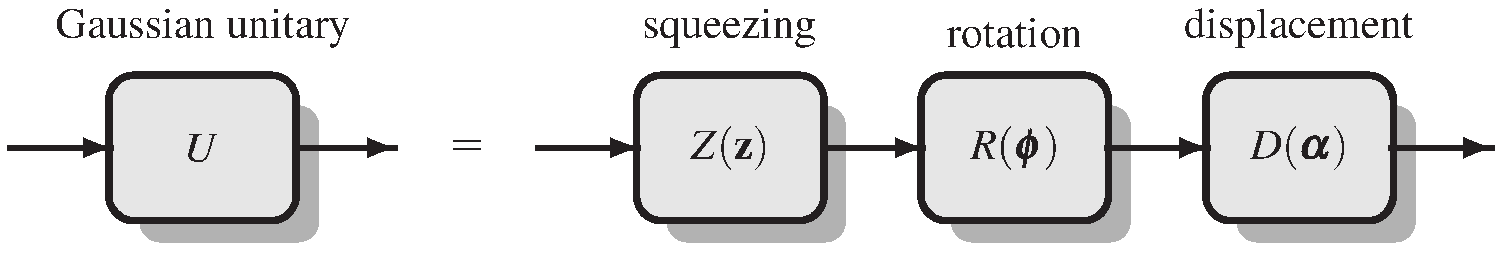
The importance of these operators is established by the following:

Theorem 2 

([9]). The most general Gaussian unitary is given by the combination of the three fundamental Gaussian unitaries $D\left(\mathit{\alpha }\right)$, $Z\left(\mathbf{z}\right)$, and $R\left(\mathit{\varphi }\right)$, cascaded in any arbitrary order, that is,

$$Z\left(\mathbf{z}\right)D\left(\mathit{\alpha }\right)R\left(\mathit{\varphi }\right),R\left(\mathit{\varphi }\right)D\left(\mathit{\alpha }\right)Z\left(\mathbf{z}\right),\mathrm{etc}.$$

(23)

This important theorem, illustrated in Figure 2 for the cascade $D\left(\mathit{\alpha }\right)R\left(\mathit{\varphi }\right)Z\left(\mathbf{z}\right)$, was proved by Ma and Rhodes [9] using the Lie algebra. Note that we can apply a few switching rules to change the order of the FGUs, with appropriate modifications of the parameters. In words, (23) can be written as six distinct orders. In the following, we refer to the order indicated in (10) and in Figure 2.

Parameter budget. Theorem 2 states that the specification of an arbitrary Gaussian unitary in the n mode is provided by: an n–size complex vector $\mathit{\alpha }$, an $n\times n$ Hermitian matrix $\mathit{\varphi }$, and an $n\times n$ complex symmetric matrix $\mathbf{z}$. This is in agreement with the budget (12).

The matrices $(\mathit{\alpha },\mathit{\varphi },\mathbf{z})$, which we call FGU parameters, carry the same information as the matrix representation $(\mathbf{H},\mathbf{h})$ of the Hamiltonians.

5.1. Hamiltonians of the FGUs

By an inspection of (20)–(22), we obtain the Hamiltonians of the FGUs and their matrix representation, as collected in the following

Table 1. Matrix representation of Hamiltonians of the FGUs.

Displacement	Rotation	Squeezing
$\mathbf{H}=\mathbf{0}$	$\mathbf{H}=\left[\begin{array}{cc}-\mathit{\varphi }& \mathbf{0}\\ \mathbf{0}& -{\mathit{\varphi }}^{\mathrm{T}}\end{array}\right]$	$\mathbf{H}=\left[\begin{array}{cc}\mathbf{0}& i\mathbf{z}\\ -i\overline{\mathbf{z}}& \mathbf{0}\end{array}\right]$
$\mathbf{h}=\left[\begin{array}{c}\mathit{\alpha }\\ \overline{\mathit{\alpha }}\end{array}\right]$	$\mathbf{h}=\mathbf{0}$	$\mathbf{h}=\mathbf{0}$

.

A comment is needed for rotation: The Gaussian unitary of rotation is given by (21), where $\mathit{\varphi }$ is a Hermitian matrix. The corresponding Hamiltonian $H=-{\mathbf{a}}^{\ast }\mathit{\varphi }\mathbf{a}$ is not in the standard form (21), but using the commutation condition, one finds

$$\begin{array}{cc}\hfill H=& -{\mathbf{a}}^{\ast }\mathit{\varphi }\mathbf{a}=-\sum _{m,n}{a}_m^{\ast }{a}_n{\mathit{\varphi }}_{mn}=-\frac{1}{2}\left[\sum _{m,n}(a_m^{\ast }{a}_n{\mathit{\varphi }}_{mn}+(a_m{a}_n^{\ast }-{\delta }_{mn}){\overline{\mathit{\varphi }}}_{nm}\right]\hfill \end{array}$$

(24)

$$\begin{array}{cc}=\hfill & -\frac{1}{2}\left[\sum _{m,n}{a}_m^{\ast }{a}_n{\mathit{\varphi }}_{mn}+\sum _{m,n}{a}_m{a}_n^{\ast }{\overline{\mathit{\varphi }}}_{nm}-Tr\left[\mathit{\varphi }\right]\right]\hfill \end{array}$$

(25)

that is,

$$H=-\frac{1}{2}{\xi }^{\ast }\mathbf{H}\xi -\frac{1}{2}Tr\left[\mathit{\varphi }\right]\mathrm{with}\mathbf{H}=\left[\begin{array}{cc}\mathit{\varphi }& \mathbf{0}\\ \mathbf{0}& \overline{\mathit{\varphi }}\end{array}\right].$$

(26)

In the application of the Hadamard lemma (in the next section), $\frac{1}{2}Tr\left[\mathit{\varphi }\right]$ disappears. Hence, the Hamiltonian can be written in the standard form (8) with the matrix $\mathbf{H}$ indicated in the Table 1.

The squeeze operator is given by (22) and is specified by the squeeze matrix $\mathbf{z}$, which is complex symmetric. To proceed, it is necessary to obtain the polar decomposition $\mathbf{z}=\mathbf{r}{e}^{i\theta }$, where $\mathbf{r}$ is Hermitian and $\theta$ is Hermitian and symmetric.

5.2. Complex Symplectic Matrices of the FGUs

For each FGU, using the expressions of H in (18), one can obtain the Bogoliubov matrices $(\mathbf{E},\mathbf{F},{\mathbf{s}}_1)$. The explicit evaluation was made in [9], and the result is collected in the following

Table 2. Bogoliubov matrices of the FGUs.

Displacement	Rotation	Squeezing
E = 0	$\mathbf{E}=e^{i\mathit{\varphi }}$	$\mathbf{E}=cosh\left(\mathbf{r}\right)$
F = 0	$\mathbf{F}=\mathbf{0}$	$\mathbf{F}=sinh\left(\mathbf{r}\right)e^{i\theta }$
${\mathbf{s}}_1=i\mathrm{\Omega }\mathit{\alpha }$	${\mathbf{s}}_1=\mathbf{0}$	${\mathbf{s}}_1=\mathbf{0}$

:

Using the relations of Table 2 for the cascade $D\left(\mathit{\alpha }\right)R\left(\mathit{\varphi }\right)Z\left(\mathbf{z}\right)$, we obtain the Bogoliubov matrices of an arbitrary Gaussian unitary.

Proposition 1. 

The Bogoliubov matrices of the most general Gaussian unitary synthesized by the cascade $D\left(\mathit{\alpha }\right)R\left(\mathit{\varphi }\right)Z\left(\mathbf{z}\right)$ are expressed, in terms of the FGU parameters, as

$$\mathbf{E}=cosh\left(\mathbf{r}\right)e^{i\mathit{\varphi }},\mathbf{F}=sinh\left(\mathbf{r}\right)e^{i\theta }{e}^{-i{\mathit{\varphi }}^{\mathrm{T}}},\mathbf{s}=i\mathit{\alpha }$$

(27)

and globally as

$$\mathbf{S}=\left[\begin{array}{cc}cosh\left(\mathbf{r}{e}^{i\mathit{\varphi }}\right)& sinh\left(\mathbf{r}\right)e^{i\theta }{e}^{-i{\mathit{\varphi }}^{\mathrm{T}}}\\ sinh\left({\mathbf{r}}^{\mathrm{T}}\right)e^{i{\theta }^{\mathrm{T}}}{e}^{i\mathit{\varphi }}& cosh\left({\mathbf{r}}^{\mathrm{T}}\right)e^{-i{\mathit{\varphi }}^{\mathrm{T}}}\end{array}\right],\mathbf{s}=i\mathrm{\Omega }\left[\begin{array}{c}\mathit{\alpha }\\ \overline{\mathit{\alpha }}\end{array}\right].$$

(28)

Parameter budget. Theorem 1 allows us to state that a Gaussian unitary can be specified by the parameters appearing in the symplectic transformation.Now, the essential specification is provided by the $n\times n$ complex matrices $\mathbf{E}$ and $\mathbf{F}$ and an n–size complex vector ${\mathbf{s}}_1$. The constrains (17) state that the matrix $\mathbf{E}{\mathbf{F}}^{\mathrm{T}}$ is symmetric and that the matrix $\mathbf{E}{\mathbf{E}}^{\ast }-\mathbf{F}{\mathbf{F}}^{\ast }$ is Hermitian. Thus, we find the same budget, given by (12), seen in the previous specifications. On the other hand, it is easy to check that the FGU parameters $(\mathit{\alpha },\mathit{\varphi },\mathbf{z})$ also have the same budget in terms of real variables.

5.3. The Real Symplectic Transformation

From the complex symplectic transformation, we can easily obtain the real symplectic transformation, which refers to quadrature operators. While the complex symplectic transformation has the form $\xi \to \mathbf{S}\xi +\mathbf{s}$, the real symplectic transformation reads $\mathbf{\eta }\to {\mathbf{S}}_0\mathbf{\eta }+{\mathbf{s}}_0$, where

$$\xi :=\left[\begin{array}{c}\mathbf{a}\\ {\mathbf{a}}_{\ast }\end{array}\right],\mathbf{\eta }=\left[\begin{array}{c}\mathbf{q}\\ \mathbf{p}\end{array}\right].$$

(29)

Then, considering the relations $q_k=(a_k+a_k^{†})/\sqrt{2}$, $p_k=-i(a_k-a_k^{†})/\sqrt{2}$, we find

$${\mathbf{S}}_0=\mathbf{L}\mathbf{S}{\mathbf{L}}^{\ast },{\mathbf{s}}_0=\mathbf{L}\mathbf{s}\mathrm{with}\mathbf{L}=\frac{1}{\sqrt{2}}\left[\begin{array}{cc}\mathbf{I}& \mathbf{I}\\ -i\mathbf{I}& i\mathbf{I}\end{array}\right]$$

(30)

and explicitly

$${\mathbf{S}}_0=\left[\begin{array}{cc}\Re (\mathbf{E}+\mathbf{F})& -\Im (\mathbf{E}-\mathbf{F})\\ \Im (\mathbf{E}+\mathbf{F})& \Re (\mathbf{E}-\mathbf{F})\end{array}\right],{\mathbf{s}}_0=\sqrt{2}\left[\begin{array}{c}\Re {\mathbf{s}}_1\\ \Im {\mathbf{s}}_1\end{array}\right]$$

(31)

The symplectic condition becomes   

$${\mathbf{S}}_0{\mathrm{\Omega }}_0{\mathbf{S}}_0^{\mathrm{T}}={\mathrm{\Omega }}_0\mathrm{with}{\mathrm{\Omega }}_0:=\frac{1}{2}\left[\begin{array}{cc}\mathbf{0}& \mathbf{I}\\ -\mathbf{I}& \mathbf{0}\end{array}\right].$$

(32)

Considering that the matrix $\mathbf{L}$ is unitary, the inverse relation results in

$$\mathbf{S}={\mathbf{L}}^{\ast }{\mathbf{S}}_0\mathbf{L}$$

(33)

6. Hamiltonians from Symplectic Transformations

Theorem 1 states that the relation of the Hamiltonian to the symplectic is: $(\mathbf{H},\mathbf{h})\to (\mathbf{S},\mathbf{s})$. Now we want to find the inverse relation $(\mathbf{S},\mathbf{s})\to (\mathbf{H},\mathbf{h})$. In principle, the inversion of the exponential is provided by the logarithm, which allows us to obtain the Hamiltonian from the symplectic matrix.

Proposition 2. 

The Hamiltonian to Bogoliubov relation $(\mathbf{S},\mathbf{s})\to (\mathbf{H},\mathbf{h})$ is

$$\mathbf{H}=log\left(\mathbf{S}\right),\mathbf{h}=-i\mathrm{\Omega }\mathbf{s}$$

(34)

The problem is that the logarithm of a matrix is not as simple as the exponential, in particular regarding its uniqueness. Hence, we find it convenient to elaborate on this topic. Given a matrix $\mathbf{A}\in {\mathbb{C}}^{n\times n}$, another matrix $\mathbf{B}\in {\mathbb{C}}^{n\times n}$ is said to be a matrix logarithm of $\mathbf{A}$, symbolized $log\left(\mathbf{A}\right)$, if $e^{\mathbf{B}}=\mathbf{A}$. Often, matrix logarithms are not unique like logarithms of complex numbers. Their uniqueness is ensured by the following theorem [11].

Theorem 3 

(principal logarithm). If $\mathbf{A}\in {\mathbb{C}}^{n\times n}$ has no eigenvalues on ${\mathbb{R}}_{-}$ there is a unique logarithm $\mathbf{B}$, whose eigenvalues lie in the strip $\{x:-\pi <\Im (z)<\pi \}$. We refer to $\mathbf{B}$ as the principal logarithm of $\mathbf{A}$. If $\mathbf{A}$ is real, the principal logarithm is real.

As regards the explicit evaluation of $log\left(\mathbf{S}\right)$, we remark that $\mathbf{S}$ is not a normal matrix, and therefore it is not diagonalizable, so the standard method of a function of a matrix based on the eigendecomposition cannot be applied. This is a difference with respect to the matrix $\mathbf{H}$, which is Hermitian. For a non-diagonalizable matrix, two equivalent methods are available: the Jordan decomposition and the the Lagrange–Hermite (LH) method (see the book by Higham [11]). We chose the LH method because it allows us to handle the matrices at block levels. In this method, the matrix function is defined by the polynomial

$$f\left(\mathbf{A}\right)=\sum _{i=0}^{n-1}{d}_i{\mathbf{A}}^i.$$

(35)

where n is the order of the matrix and the coefficients $d_i$ take different expressions in dependence of the multiplicities of the eigenvalues and of the function $f\left(t\right)$ (see Appendix A.1).

In the present context, the principal logarithm is related to the eigenvalues of $\mathbf{S}$, for which, in Appendix A.2, we prove:

Proposition 3. 

The eigenvalues of a complex symplectic matrix $\mathbf{S}$ are couples $(\lambda ,1/\lambda )$ of real numbers or quadruples $(\lambda ,\overline{\lambda },1/\lambda ,1/\overline{\lambda })$ of complex non-real numbers.

Combination of Two Exponentials in a Single Exponential

Consider the relation

$$\mathbf{S}={\mathbf{S}}_{\mathrm{sq}}{\mathbf{S}}_{\mathrm{rot}}=e^{-i\mathrm{\Omega }{\mathbf{H}}_{\mathrm{sq}}}{e}^{-i\mathrm{\Omega }{\mathbf{H}}_{\mathrm{rot}}}$$

(36)

where ${\mathbf{H}}_{\mathrm{sq}}$ and ${\mathbf{H}}_{\mathrm{rot}}$ are given in Table 1. In general,

$$e^{-i\mathrm{\Omega }{\mathbf{H}}_{\mathrm{sq}}}{e}^{-i\mathrm{\Omega }{\mathbf{H}}_{\mathrm{rot}}}\ne e^{-i\mathrm{\Omega }{\mathbf{H}}_{\mathrm{sq}}-i\mathrm{\Omega }{\mathbf{H}}_{\mathrm{rot}}}$$

(37)

but we can evaluate the product

$$\mathbf{S}={\mathbf{S}}_{\mathrm{sq}}{\mathbf{S}}_{\mathrm{rot}}=\left[\begin{array}{cc}{\mathbf{E}}_{\mathrm{sq}}& {\mathbf{F}}_{\mathrm{sq}}\\ {\overline{\mathbf{F}}}_{\mathrm{sq}}& {\overline{\mathbf{E}}}_{\mathrm{sq}}\end{array}\right]\left[\begin{array}{cc}{\mathbf{E}}_{\mathrm{rot}}& {\mathbf{F}}_{\mathrm{rot}}\\ {\overline{\mathbf{F}}}_{\mathrm{sq}}& {\overline{\mathbf{E}}}_{\mathrm{sq}}\end{array}\right]$$

(38)

and use the identity $\mathbf{S}=e^{log\mathbf{S}}$.

Proposition 4. 

A general Gaussian unitary can be expressed by a single Hamiltonian as $U=e^{-i\mathrm{\Omega }\mathbf{H}}$, where

$$\mathbf{H}=i\mathrm{\Omega }log\left({\mathbf{S}}_{\mathrm{sq}}{\mathbf{S}}_{\mathrm{rot}}\right)$$

(39)

with ${\mathbf{S}}_{\mathrm{sq}}{\mathbf{S}}_{\mathrm{rot}}$ given by (38). Once evaluated, $\mathbf{H}$ (36) becomes

$$e^{-i\mathrm{\Omega }{\mathbf{H}}_{\mathrm{sq}}}{e}^{-i\mathrm{\Omega }{\mathbf{H}}_{\mathrm{rot}}}=e^{-i\mathrm{\Omega }\mathbf{H}}$$

(40)

that is, the product of two noncommutable exponentials are combined in a single exponential.

For the evaluation of the matrix log in (39), we use the LH formula.

7. Application to the Single Mode

We check the previous theory in the single mode, which leads to simple results. The matrix representations of the Hamiltonian are given by

$$\mathbf{H}=\left[\begin{array}{cc}A& B\\ \overline{B}& \overline{A}\end{array}\right],\mathbf{h}=\left[\begin{array}{c}h\\ \overline{h}\end{array}\right].$$

(41)

where $A,B,h\in \mathbb{C}$. The Bogoliubov parameters are

$$\mathbf{S}=\left[\begin{array}{cc}E& F\\ \overline{F}& \overline{E}\end{array}\right],\mathbf{s}=\left[\begin{array}{c}s\\ \overline{s}\end{array}\right]$$

(42)

with $E,F,s\in \mathbb{C}$ scalars, which verify the condition $E{E}^{\ast }-F{F}^{\ast }=1$. The FGU parameters are $(z=r{e}^{i\theta },\mathit{\varphi },\mathit{\alpha }$) with $r\ge 0$ and $\theta ,\mathit{\varphi }\in \mathbb{R},\mathit{\alpha }\in \mathbb{C}$. Then, the complex symplectic parameters become

$$\mathbf{S}=\left[\begin{array}{cc}cosh\left(r\right)e^{i\mathit{\varphi }}& sinh\left(r\right)e^{i(\theta +\mathit{\varphi })}\\ sinh\left(r\right)e^{-i(\theta +\mathit{\varphi })}& cosh\left(r\right)e^{-i\mathit{\varphi }}\end{array}\right],\mathbf{s}=i\mathrm{\Omega }\mathbf{h}=i\left[\begin{array}{c}\mathit{\alpha }\\ -\overline{\mathit{\alpha }}\end{array}\right].$$

(43)

We give the formulas for the function $f\left(\mathbf{A}\right)$ of a $2\times 2$ complex matrix $\mathbf{A}$ needed in the single mode. The LH formula gives

$$f\left(\mathbf{A}\right)=d_0{\mathbf{I}}_2+d_1\mathbf{A}$$

(44)

where the coefficients are evaluated from the eigenvalues ${\lambda }_{1,2}$ of $\mathbf{A}$ (see Appendix A.1)

$$\begin{array}{cc}\hfill & d_0=f\left({\lambda }_1\right)-{\lambda }_1{f}^{\prime }\left({\lambda }_1\right)d_1=f^{\prime }\left({\lambda }_1\right)\mathrm{for}{\lambda }_1={\lambda }_2\hfill \end{array}$$

(45)

$$\begin{array}{cc}\hfill & d_0=\frac{{\lambda }_{1}f\left({\lambda }_2\right)-{\lambda }_{2}f\left({\lambda }_1\right)}{{\lambda }_1-{\lambda }_2}{d}_1=\frac{f\left({\lambda }_1\right)-f\left({\lambda }_2\right)}{{\lambda }_1-{\lambda }_2}\mathrm{for}{\lambda }_1\ne {\lambda }_2\hfill \end{array}$$

(46)

7.1. Hamiltonian to Symplectic $(\mathbf{H},\mathbf{h})\to (\mathbf{S},\mathbf{s})$

The basic relation is $\mathbf{S}=e^{-i\mathrm{\Omega }\mathbf{H}}$. The eigenvalues of $-i\mathrm{\Omega }\mathbf{H}$ are ${\lambda }_{1,2}=\mp \sqrt{{\left|B\right|}^2-A^2}$. Then, the LH formula gives

$$\mathbf{S}=d_0{\mathbf{I}}_2+d_1(-i\mathrm{\Omega }\mathbf{H})$$

(47)

where   

$$\begin{array}{cc}\hfill & d_0=e^{{\lambda }_1}-{\lambda }_1{e}^{{\lambda }_1},d_1=e^{{\lambda }_1}{\lambda }_1={\lambda }_2\hfill \end{array}$$

(48)

$$\begin{array}{cc}\hfill & d_0=\frac{e^{{\lambda }_2}{\lambda }_1-e^{{\lambda }_1}{\lambda }_2}{{\lambda }_1-{\lambda }_2},d_1=\frac{e^{{\lambda }_1}-e^{{\lambda }_2}}{{\lambda }_1-{\lambda }_2}{\lambda }_1\ne {\lambda }_2.\hfill \end{array}$$

(49)

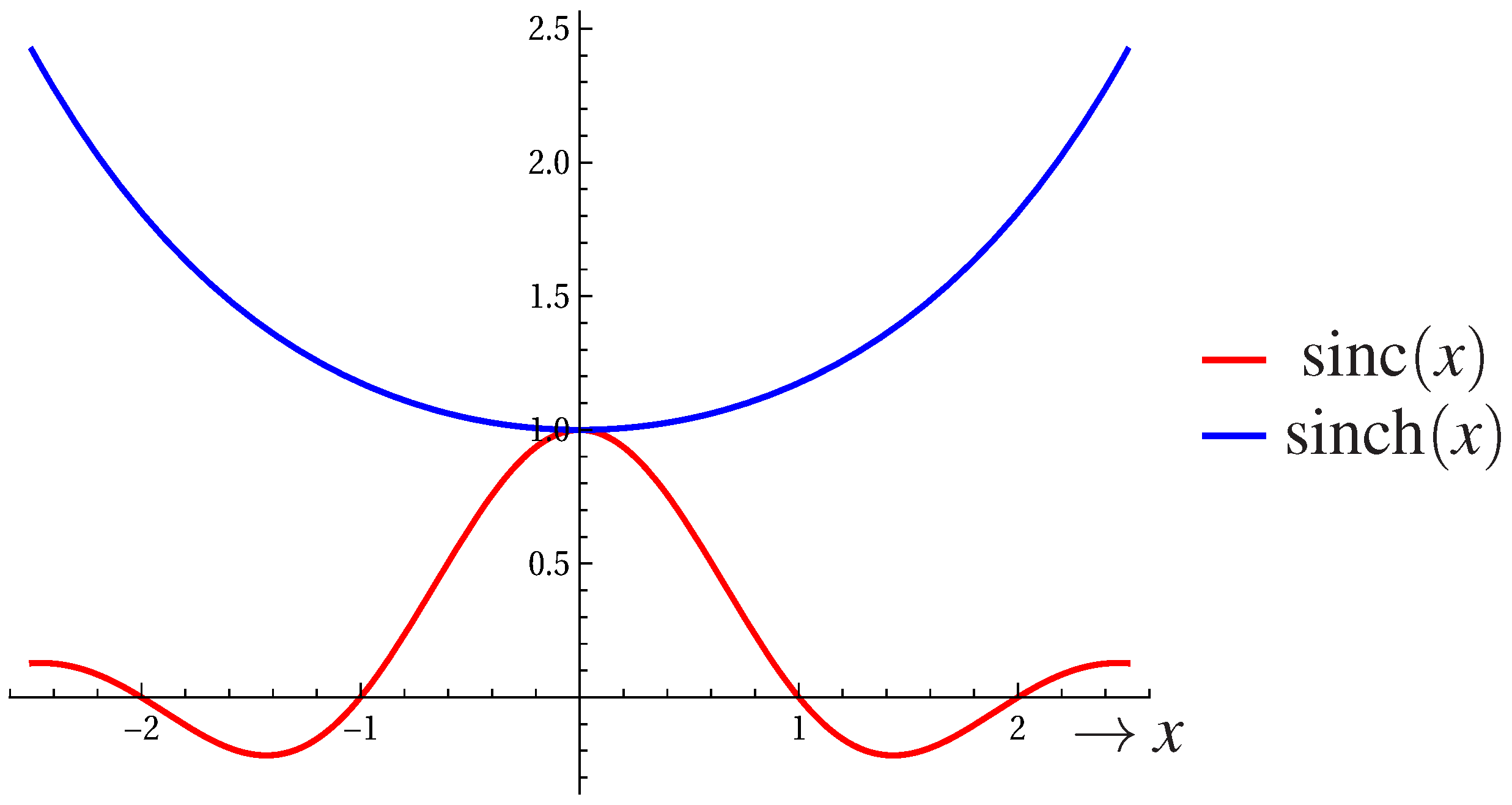
To express the Bogoliubov parameters, we introduce the functions $\mathrm{sinc}\left(x\right):=sin\left(x\right)/x$ and $\mathrm{sinch}\left(x\right):=sinh\left(x\right)/x$, which are illustrated in Figure 3.

Proposition 5. 

In the single mode the relation of the Hamiltonian to the symplectic $(A,B,h)\to (E,F,s)$ is given by

$$E=cosh\left(L\right)-iA\mathrm{sinch}\left(L\right),F=iB\mathrm{sinch}\left(L\right),s=ih$$

(50)

where $L=\sqrt{{\left|B\right|}^2-A^2}$.

Note that E and F depend only on $A^2$, and without restriction we assume $A\ge 0$. Note also that for $\left|B\right|<A$, the square root L becomes imaginary, $L=i\sqrt{A^2-{\left|B\right|}^2}$, but, considering the identities $cosh\left(iz\right)=cos\left(z\right)$ and $\mathrm{sinch}\left(iz\right)=\mathrm{sinc}\left(z\right)$, we can see that (50) also holds in this case.

7.2. Symplectic to Hamiltonian: $(\mathbf{S},\mathbf{s})\to (\mathbf{H},\mathbf{h})$

In the single mode, the symplectic parameters are scalars,

$$E=cosh\left(r\right)e^{i\mathit{\varphi }},F=sinh\left(r\right)e^{i\theta }{e}^{-i\mathit{\varphi }},s=\mathit{\alpha }.$$

(51)

Proposition 2 gives $\mathbf{H}=i\mathrm{\Omega }log\left(\mathbf{S}\right)$ and the LH formula reads $log\left(\mathbf{S}\right)=d_0{I}_2+d_1\mathbf{S}$. The coefficients $d_0$ and $d_1$ are evaluated in terms of the eigenvalues ${\lambda }_{1,2}$ of $\mathbf{S}$, specifically

$$\begin{array}{cc}\hfill & d_0=log\left({\lambda }_1\right)-1,d_1=\frac{1}{{\lambda }_1}\mathrm{for}{\lambda }_1={\lambda }_2\hfill \end{array}$$

(52)

$$\begin{array}{cc}\hfill & d_0=\frac{{\lambda }_{1}log\left({\lambda }_2\right)-{\lambda }_{2}log\left({\lambda }_1\right)}{{\lambda }_1-{\lambda }_2},d_1=\frac{log\left({\lambda }_1\right)-log\left({\lambda }_2\right)}{{\lambda }_1-{\lambda }_2}\mathrm{for}{\lambda }_1\ne {\lambda }_2.\hfill \end{array}$$

(53)

Hence,

$$\mathbf{H}=d_0{\mathbf{I}}_2+d_{1}i\mathrm{\Omega }\mathbf{S}=\left[\begin{array}{cc}i(d_0+E{d}_1)& iF{d}_1\\ -i\overline{F}{d}_1& -i(d_0+\overline{E}{d}_1)\end{array}\right]=\left[\begin{array}{cc}A& B\\ \overline{B}& \overline{A}\end{array}\right]$$

(54)

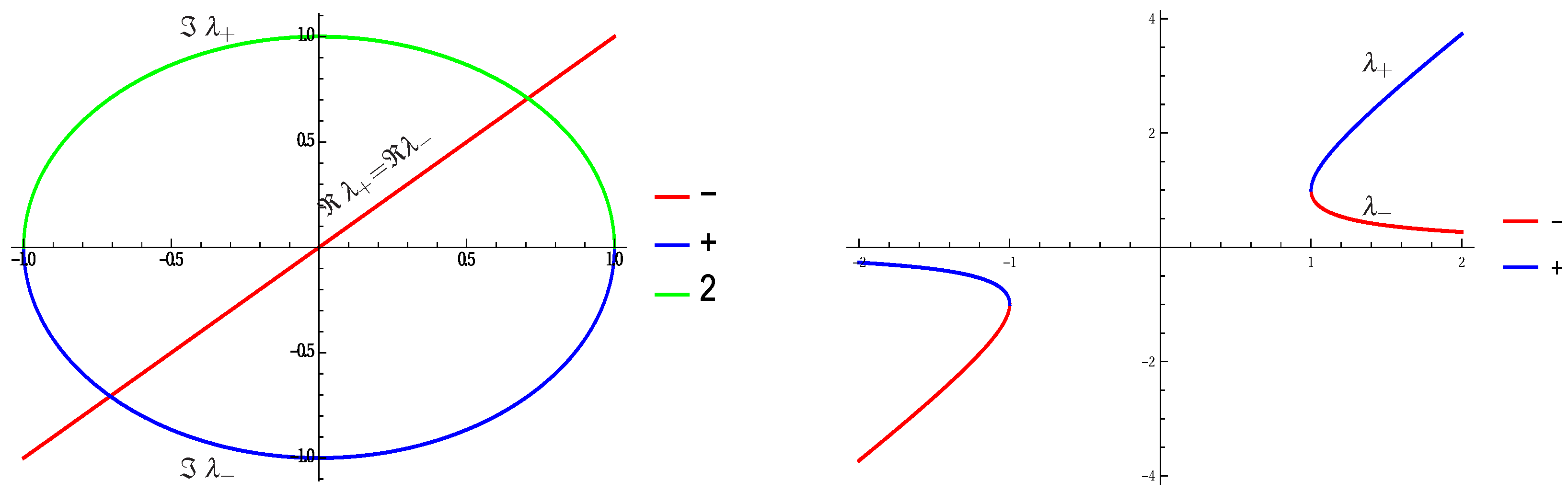
The eigenvalues of $\mathbf{S}$ are given by

$${\lambda }_{-}=\Re \left(E\right)-\sqrt{\Re {\left(E\right)}^2-1},{\lambda }_{+}=\Re \left(E\right)+\sqrt{\Re {\left(E\right)}^2-1}$$

(55)

where the condition $E{E}^{\ast }-F{F}^{\ast }=1$ has been used. Thus, the eigenvalues ${\lambda }_{1,2}={\lambda }_{\mp }$ depend only on $\Re \left(E\right)$, and are illustrated in Figure 4 versus $\Re \left(E\right)$. They verify the condition ${\lambda }_{-}=1/{\lambda }_{+}$, in agreement with Proposition 2.

We proceed with the case $|\Re (E\left)\right|\ne 1$. As shown in Figure 4, the eigenvalues are real for $|\Re (E)>1$ and are complex conjugate for $|\Re (E)<1$. The evaluation of the coefficients do not meet any problems, even with complex eigenvalues, provided that the principal value of the logarithm is taken, e.g., $log\left(i\right)=i\pi /2$.

Proposition 6. 

In the single mode, the Bogoliubov to symplectic relation $(E,F,s)\to (A,B,h)$ for $E\ne \mp 1$ is given by

$$A=\frac{\Im \left(E\right)}{{\lambda }_{+}-{\lambda }_{-}}log\frac{{\lambda }_{-}}{{\lambda }_{+}},B=-i\frac{F}{{\lambda }_{+}-{\lambda }_{-}}log\frac{{\lambda }_{-}}{{\lambda }_{+}}$$

(56)

where ${\lambda }_{\mp }=\Re \left(E\right)\mp \sqrt{\Re {\left(E\right)}^2-1}$ are the eigenvalues of $\mathbf{S}$.

We recall that $E=cosh\left(r\right)e^{i\mathit{\varphi }}$ and $F=sinh\left(r\right)e^{i(\theta -\mathit{\varphi })}$. Then, (56) can be written in the form

$$A=sin\left(\mathit{\varphi }\right)cosh\left(r\right)p\left(M\right),B=-i{e}^{i\theta -i\mathit{\varphi }}sinh\left(r\right)p\left(M\right)$$

(57)

where $M=\Re \left(E\right)=cos\left(\mathit{\varphi }\right)cosh\left(r\right)$ and

$$p\left(M\right)=\frac{1}{\sqrt{M^2-1}}log\left[M-\sqrt{M^2-1}\right]$$

(58)

This function is critical for the presence of log; it is discussed in detail in Appendix A.3, where we find

$$p\left(M\right)=\left\{\begin{array}{cc}\frac{1}{\sqrt{M^2-1}}\left\{log\left[-M+\sqrt{M^2-1}\right]+i\pi \right\}\hfill & \mathrm{for} \left|M\right|<1\hfill \\ \frac{1}{\sqrt{M^2-1}}log\left[M-\sqrt{M^2-1}\right]\hfill & \mathrm{for} M>1\hfill \end{array}\right.$$

(59)

The plot of the function $p\left(M\right)$ is shown in Figure 5.

8. Application to the Two Mode

The explicit evaluation seen for the single mode can be extended to a general two-mode Gaussian unitary, where the matrices involved are $4\times 4$, and the LH formula reads

$$f\left(\mathbf{A}\right)=\sum _{i=0}^3{d}_i{\mathbf{A}}^i.$$

(60)

The coefficients take different expressions in dependence of the multiplicities of the eigenvalues of $\mathbf{A}$ and of the function $f\left(t\right)$. In Appendix A.1, the general expressions of the coefficients $d_i$ are collected, and in this section, they are applied both to $\mathbf{H}\to \mathbf{S}$ and to $\mathbf{S}\to \mathbf{H}$ cases. The advantage of the LH method is that it can be applied at block levels (in the present case the blocks are $2\times 2$).

The matrix representation $(\mathbf{H},\mathbf{h})$ of the Hamiltonian is

$$\mathbf{A}=\left[\begin{array}{cc}{a}_{11}& a_{12}\\ {\overline{a}}_{12}& a_{22}\end{array}\right],\mathbf{B}=\left[\begin{array}{cc}{b}_{11}& b_{12}\\ b_{12}& b_{22}\end{array}\right],\mathbf{h}=\left[\begin{array}{c}{h}_1\\ h_2\end{array}\right]$$

(61)

with $a_{11},a_{22}\in \mathbb{R}$, $a_{12},b_{11},b_{12},b_{22}$, $h_1,h_2\in \mathbb{C}$. The blocks of the symplectic parameters are

$$\mathbf{E}=\left[\begin{array}{cc}{e}_{11}& e_{12}\\ e_{12}& e_{22}\end{array}\right],\mathbf{F}=\left[\begin{array}{cc}{f}_{11}& f_{12}\\ f_{12}& f_{22}\end{array}\right]$$

(62)

which verify the conditions (17). The FGU triplet has the structure

$$\mathbf{z}=\left[\begin{array}{cc}{z}_{11}& z_{12}\\ z_{12}& z_{22}\end{array}\right],\mathit{\varphi }=\left[\begin{array}{cc}{\mathit{\varphi }}_{11}& {\mathit{\varphi }}_{12}\\ \overline{{\mathit{\varphi }}_{12}}& {\mathit{\varphi }}_{22}\end{array}\right],\mathit{\alpha }=\left[\begin{array}{c}{\mathit{\alpha }}_1\\ {\mathit{\alpha }}_2\end{array}\right]$$

(63)

8.1. Hamiltonian to Symplectic $(\mathbf{H},\mathbf{h})\to (\mathbf{S},\mathbf{s})$

The first step is the evaluation of the the matrix exponential $\mathbf{S}=exp[-i\mathrm{\Omega }\mathbf{H}]$, where $\mathbf{H}$ and $\mathbf{S}$ are $4\times 4$. With Mathematica, we obtain a formula for $\mathbf{S}$, but its length is more than twenty pages, so is useless. It is more convenient to use the LH formula, which reads

$$\mathbf{S}=e^{\mathbf{K}}=\sum _{m=0}^3{d}_m{\mathbf{K}}^m\mathrm{with}{\mathbf{K}}^m={(-i\mathrm{\Omega }\mathbf{H})}^m$$

(64)

now we can calculate the blocks $\mathbf{E}$ and $\mathbf{F}$ of $\mathbf{S}$ in terms of the blocks $\mathbf{A}$ and $\mathbf{B}$ by evaluating the powers of $\mathbf{K}$. We obtain

$$\mathbf{E}=\sum _{m=0}^3{d}_m{\mathbf{E}}_m,\mathbf{F}=\sum _{m=0}^3{d}_m{\mathbf{F}}_m$$

(65)

where

$$\begin{array}{cc}\hfill & {\mathbf{F}}_0=\mathbf{0},{\mathbf{F}}_1=-i\mathbf{B},{\mathbf{F}}_2=\mathbf{B}\overline{\mathbf{A}}-\mathbf{A}\mathbf{B},{\mathbf{F}}_3=-i\left[\mathbf{A}(\mathbf{B}\overline{\mathbf{A}}-\mathbf{A}\mathbf{B})+\mathbf{B}(\mathbf{B}\overline{\mathbf{B}}-{\overline{\mathbf{A}}}^2)\right]\hfill \end{array}$$

(66)

$$\begin{array}{cc}\hfill & {\mathbf{E}}_0=\mathbf{I},{\mathbf{E}}_1=-i\mathbf{A},{\mathbf{E}}_2=\mathbf{B}\overline{\mathbf{B}}-{\mathbf{A}}^2,{\mathbf{E}}_3=-i\left[\mathbf{A}(\mathbf{B}\overline{\mathbf{B}}-{\mathbf{A}}^2)+\mathbf{B}(\overline{\mathbf{B}}\mathbf{A}-\overline{\mathbf{B}}\overline{\mathbf{A}})\right]\hfill \end{array}$$

(67)

The coefficients $d_m$ depend on the eigenvalues of $\mathbf{S}$, which are more conveniently calculated from the characteristic polynomial $C\left(\lambda \right)=det(\mathbf{K}-\lambda \mathbf{I})$. In Appendix A.4, we find the following two cases:

Distinct eigenvalues. The eigenvalues are opposite in pairs, say ${\lambda }_{1,2}=\mp p$ and ${\lambda }_{3,4}=\mp q$, with

$$p=\frac{1}{\sqrt{2}}\sqrt{-c_2-\sqrt{c_2^2-4c_0}},q=\frac{1}{\sqrt{2}}\sqrt{-c_2+\sqrt{c_2^2-4c_0}}.$$

(68)

Then the coefficients $d_m$ take the simple expressions given by (68).

$$\begin{array}{cc}\hfill & d_0=\frac{p^{2}cosh\left(q\right)-q^{2}cosh\left(p\right)}{p^2-q^2},d_1=\frac{p^{3}sinh\left(q\right)-q^{3}sinh\left(p\right)}{p^{3}q-p{q}^3}\hfill \end{array}$$

(69)

$$\begin{array}{cc}\hfill & d_2=\frac{cosh\left(p\right)-cosh\left(q\right)}{p^2-q^2},d_3=\frac{qsinh\left(p\right)-psinh\left(q\right)}{p^{3}q-p{q}^3.}\hfill \end{array}$$

(70)

Eigenvalues coincident in pairs. The eigenvalues have the form ${\lambda }_{12}=\mp p$, ${\lambda }_{3,4}=\mp p$, where $p=\frac{1}{\sqrt{2}}\sqrt{-c_2}$. The coefficients take the expressions

$$\begin{array}{cc}\hfill & d_0=cosh\left(p\right)-\frac{1}{2}psinh\left(p\right),d_1=\frac{3sinh\left(p\right)}{2p}-\frac{cosh\left(p\right)}{2}\hfill \end{array}$$

(71)

$$\begin{array}{cc}\hfill & d_2=\frac{sinh\left(p\right)}{2p},d_3=\frac{pcosh\left(p\right)-sinh\left(p\right)}{2p^3}.\hfill \end{array}$$

(72)

In conclusion, for the evaluation of $\mathbf{S}=e^{\mathbf{K}}$ in the two mode, we have to calculate the eigenvalues ${\lambda }_i$ of $\mathbf{K}$ (see Appendix A) and then we have the symplectic matrices from (65). Again, the interpolation leads to simple results, while the other methods lead to intractable formulas.

8.2. Symplectic to Hamiltonian: $(\mathbf{S},\mathbf{s})\to (\mathbf{H},\mathbf{h})$

The general formula giving the Hamiltonian representation $\mathbf{H}$ from the symplectic matrix $\mathbf{S}$ is $\mathbf{H}=i\mathrm{\Omega }log\mathbf{S}$, where the logarithm is evaluated using the LH formula, as follows

$$log\mathbf{S}==\sum _{m=0}^3{d}_m{\mathbf{S}}^m.$$

(73)

From the powers of $\mathbf{S}$, we obtain

$$\mathbf{A}=\sum _{m=0}^3{d}_m{\mathbf{A}}_m,\mathbf{B}=\sum _{m=0}^3{d}_m{\mathbf{B}}_m$$

(74)

where

$$\begin{array}{cc}\hfill & {\mathbf{A}}_0={\mathbf{I}}_2,{\mathbf{A}}_1=\mathbf{E},{\mathbf{A}}_2=+\mathbf{F}\overline{\mathbf{F}}+{\mathbf{E}}^2,{\mathbf{A}}_3=\mathbf{E}(\mathbf{F}\overline{\mathbf{F}}+{\mathbf{E}}^2)+\mathbf{F}(\overline{\mathbf{F}}\mathbf{E}+\overline{\mathbf{F}}\overline{\mathbf{E}})\hfill \end{array}$$

(75)

$$\begin{array}{cc}\hfill & {\mathbf{B}}_0=\mathbf{0},{\mathbf{B}}_1=+i\mathbf{F},{\mathbf{B}}_2=+\mathbf{F}\overline{\mathbf{E}}+\mathbf{E}\mathbf{F},{\mathbf{B}}_3=\mathbf{E}\left(\mathbf{F}\overline{\mathbf{E}}\right)+\mathbf{E}\mathbf{F})+\mathbf{F}(\mathbf{F}\overline{\mathbf{F}}+{\overline{\mathbf{E}}}^2)\hfill \end{array}$$

(76)

For the evaluation of the coefficients $d_m$, see Appendix A.5, where two cases are considered: (1) four distinct eigenvalues and (2) two coincident eigenvalues.

In conclusion, for the evaluation of $\mathbf{H}$ in the two mode, we have to calculate the eigenvalues ${\mu }_i$ of $\mathbf{S}$, and then we have the Hamiltonian matrices from (74). The interpolation method leads to simple results, while other methods lead to intractable formulas.

8.3. Example: EPR Unitary Followed by a Beam Splitter

We develop an explicit example in the two mode: a Gaussian unitary obtained as the cascade of the EPR unitary, followed by a beam splitter. The EPR (Einstein–Podolski–Rosen) unitary is a celebrated two-mode squeezer, which is very important, mainly for historical reasons [21,22]. The beam splitter (BS) is certainly a useful device and deserves separate considerations, but the matrix decomposition described in this paper can still be applied to beam splitting; it can be modeled as a two-mode rotation. We know the Bogoliubov matrices of these devices, which are given by

$${\mathbf{E}}_{\mathrm{EPR}}=\left[\begin{array}{cc}cosh\left(r\right)& 0\\ 0& cosh\left(r\right)\end{array}\right],{\mathbf{F}}_{\mathrm{EPR}}=\left[\begin{array}{cc}0& sinh\left(r\right)e^{i\theta }\\ sinh\left(r\right)e^{-i\theta }& 0\end{array}\right],r,\theta \in \mathbb{R}$$

(77)

$${\mathbf{E}}_{\mathrm{BS}}=\left[\begin{array}{cc}cos\left(\beta \right)& sin\left(\beta \right)\\ -sin\left(\beta \right)& cos\left(\beta \right)\end{array}\right],{\mathbf{F}}_{\mathrm{BS}}=\left[\begin{array}{cc}0& 0\\ 0& 0\end{array}\right],\beta \in \mathbb{R}$$

(78)

and we wish to evaluate the Hamiltonian that produces this cascade.

To this end, we construct the global symplectic matrix

$$\mathbf{S}={\mathbf{S}}_{\mathrm{BS}}{\mathbf{S}}_{\mathrm{EPR}}=\left[\begin{array}{cc}{\mathbf{E}}_{\mathrm{BS}}& {\mathbf{F}}_{\mathrm{BS}}\\ {\overline{\mathbf{F}}}_{\mathrm{BS}}& {\overline{\mathbf{E}}}_{\mathrm{BS}}\end{array}\right]\left[\begin{array}{cc}{\mathbf{E}}_{\mathrm{EPR}}& {\mathbf{F}}_{\mathrm{EPR}}\\ {\overline{\mathbf{F}}}_{\mathrm{EPR}}& {\overline{\mathbf{E}}}_{\mathrm{EPR}}\end{array}\right]$$

(79)

The matrix $\mathbf{S}$ has two distinct eigenvalues with multiplicity 2

$${\mu }_{1,2}=cos\left(\beta \right)cosh\left(r\right)\mp \frac{1}{2}\sqrt{2{cos}^2\left(\beta \right)cosh\left(2r\right)+cos\left(2\beta \right)-3}$$

(80)

The coefficients of the LH formula are

$$\begin{array}{cc}\hfill & d_0=\frac{-({\mu }_1-{\mu }_2)\left[{\mu }_1^2+{\mu }_2^2\right]+({\mu }_1-3{\mu }_2){\mu }_1^{2}log\left({\mu }_2\right)+(3{\mu }_1-{\mu }_2){\mu }_2^{2}log\left({\mu }_1\right)}{{({\mu }_1-{\mu }_2)}^3}\hfill \end{array}$$

(81)

$$\begin{array}{cc}\hfill & d_1=\frac{({\mu }_1-{\mu }_2)({\mu }_1+{\mu }_2)\left[{\mu }_1^2+{\mu }_2{\mu }_1+{\mu }_2^2\right]+6{\mu }_1^2{\mu }_2^2(log\left({\mu }_2\right)-log\left({\mu }_1\right))}{{\mu }_1{({\mu }_1-{\mu }_2)}^3{\mu }_2}\hfill \end{array}$$

(82)

$$\begin{array}{cc}\hfill & d_2=\frac{-2{\mu }_1^3+2{\mu }_2^3+3{\mu }_2({\mu }_1+{\mu }_2){\mu }_1(log\left({\mu }_1\right)-log\left({\mu }_2\right))}{{\mu }_1{({\mu }_1-{\mu }_2)}^3{\mu }_2}\hfill \end{array}$$

(83)

$$\begin{array}{cc}\hfill & d_3=\frac{{\mu }_1^2-{\mu }_2^2+2{\mu }_2{\mu }_1(log\left({\mu }_2\right)-log\left({\mu }_1\right))}{{\mu }_1{({\mu }_1-{\mu }_2)}^3{\mu }_2}\hfill \end{array}$$

(84)

8.4. Application to a Three Mode: Lossless Triple Coupler

We could formulate explicitly the theory of a three-mode Gaussian unitary, but, of course, the general formulas become long and tedious. For this reason, we develop only a specific case: the lossless triple coupler, considered by Ferraro et al. in [23] (p. 56), which is specified by the unitary matrix

$$\mathbf{W}=\frac{1}{\sqrt{3}}\left[\begin{array}{ccc}1& 1& 1\\ 1& \gamma & {\gamma }^{\ast }\\ 1& {\gamma }^{\ast }& \gamma \end{array}\right]\mathrm{with}\gamma :=W_3=e^{i2\pi /3}$$

(85)

This unitary acts on bosonic operators $\mathbf{a}={[a_1,a_2,a_3]}^{\mathrm{T}}$ as $\mathbf{a}\to \mathbf{W}\mathbf{a}$, which is a special case of the Bogoliubov transformation with matrices $\mathbf{E}=\mathbf{W},\mathbf{F}=\mathbf{0},\mathbf{d}=\mathbf{0}$, and therefore, the corresponding Gaussian unitary is a three-mode rotation operator

$$R_{(}\mathit{\varphi })=e^{i{\mathbf{a}}^{\ast }\mathit{\varphi }\mathbf{a}}$$

(86)

with phase matrix $\mathit{\varphi }$ defined implicitly by $\mathbf{W}=e^{i\mathit{\varphi }}$. The evaluation of the complex symplectic matrix is immediate, namely,

$$\mathbf{S}=\left[\begin{array}{cc}\mathbf{W}& \mathbf{0}\\ \mathbf{0}& \overline{\mathbf{W}}\end{array}\right].$$

(87)

For the evaluation of $\mathbf{H}$, considering that $\mathbf{S}$ is block diagonal, we can use the formula

$$log\left(\mathbf{S}\right)=\left[\begin{array}{cc}log\left(\mathbf{W}\right)& \mathbf{0}\\ \mathbf{0}& log\left(\overline{\mathbf{W}}\right)\end{array}\right]$$

(88)

so that it is sufficient to evaluate $log\left(\mathbf{W}\right)$, which is $3\times 3$. The LH formula for $n=3$ reads

$$log\left(\mathbf{W}\right)=d_0\mathbf{I}+d_1\mathbf{W}+d_2{\mathbf{W}}^2$$

(89)

The eigenvalues of $\mathbf{W}$ are ${\lambda }_1=+1,{\lambda }_2=-1,{\lambda }_3=i$ and the coefficients must be evaluated with $f\left(x\right)=log\left(x\right)$ and distinct eigenvalues. One finds

$$d_0=\left(-\frac{1}{4}+\frac{i}{2}\right)\pi ,d_1=-\frac{i\pi }{2},d_2=\frac{\pi }{4}$$

(90)

In conclusion

$$\mathbf{A}=log\left(\mathbf{W}\right)=\left[\begin{array}{ccc}-\frac{1}{6}i\left(\sqrt{3}-3\right)\pi & -\frac{i\pi }{2\sqrt{3}}& -\frac{i\pi }{2\sqrt{3}}\\ -\frac{i\pi }{2\sqrt{3}}& \frac{1}{12}i\left(6+\sqrt{3}\right)\pi & \frac{i\pi }{4\sqrt{3}}\\ -\frac{i\pi }{2\sqrt{3}}& \frac{i\pi }{4\sqrt{3}}& \frac{1}{12}i\left(6+\sqrt{3}\right)\pi \end{array}\right]$$

(91)

This completes the evaluation of the matrix representation of the Hamiltonian, given by

$$\mathbf{H}=\left[\begin{array}{cc}\mathbf{A}& \mathbf{0}\\ \mathbf{0}& \overline{\mathbf{A}}\end{array}\right]$$

(92)

9. Conclusions

The paper has developed the relation between the Hamiltonian and the complex symplectic representation, based on an exponential, and the inverse relation, based on a logarithm. The inverse relation, which does not seem to be available in the literature, is the critical part for the multiplicity of the logarithm of a complex matrix. However, it has clearly been developed using the Lagrange–Hermite interpolation method.

The results of the theory have been obtained explicitly for an arbitrary n mode, although applications have been limited to the single and the two modes. They can be extended to higher modes with the penalty of encountering long formulas.

We also note that the systematic application of the symplectic part to most general Gaussian unitaries seem to be new (in the literature one finds only applications to particular cases of squeezing). This possibility was achieved following the general theory of Ma and Rhodes, developed in a historical paper of 1990 [9].

The introduction of the complex symplectic matrix, instead of the traditional real symplectic matrix, merits particular attention, not only for its beauty and its perfect symmetry with Hamiltonian specification (compare Equation (1) with Equation (2)), but also for the unification it provides with the Bogoliubov specification.

The authors are currently investigating the possibility of applying the theory in this paper to a new topic: quantum communications with multimode Gaussian states, in particular with the two mode, which seems not to be considered in the literature. In this topic, the critical part is the evaluation of the inner product of the two quantum states, for which we have obtained an explicit closed-form result [24].