Numerical Simulation for COVID-19 Model Using a Multidomain Spectral Relaxation Technique

Abstract

The major objective of this work is to evaluate and study the model of coronavirus illness by providing an efficient numerical solution for this important model. The model under investigation is composed of five differential equations. In this study, the multidomain spectral relaxation method (MSRM) is used to numerically solve the suggested model. The proposed approach is based on the hypothesis that the domain of the problem can be split into a finite number of subintervals, each of which can have a solution. The procedure also converts the proposed model into a system of algebraic equations. Some theoretical studies are provided to discuss the convergence analysis of the suggested scheme and deduce an upper bound of the error. A numerical simulation is used to evaluate the approach’s accuracy and utility, and it is presented in symmetric forms.

1. Introduction

One of the most well-known illnesses today is the coronavirus disease (COVID-19) [1,2,3]. The World Health Organization (WHO) declared this illness to be a pandemic on 11 March 2020, forcing all nations, big and small, to take precautions to preserve the lives of their citizens. The spread of this pandemic disease has hurt the world’s economy. Due to this extensively disseminated pandemic illness, businesses, colleges, marketplaces, and a variety of other organizations have taken unique preventative measures. Curfews have been put in place to prevent overcrowding and the subsequent spread of disease, and both internal and external travel has been suspended for several months, according to [4]. This pandemic is dangerous because of how quickly it may spread and the different infections that people can get.

Our lives depend heavily on mathematical modeling [5,6,7,8,9,10]. According to [11], mathematical models are essential for forecasting disease outbreaks as well as for preventing and controlling outbreaks. The study of infectious diseases and the creation of efficient control methods is one of modeling’s most significant applications. There are different models, depending on the transmission technique assumptions. SIR models have been used to take into account whether a person is aware of the disease [12,13], for instance, and many other models have been used to simulate double pandemic and nonlinear occurrence rate theories [14,15,16,17]. Since the introduction of COVID-19, researchers have been developing mathematical models to better understand the pandemic’s mechanism of transmission, effect, propagation, control, and prevention as well as the effects of preventive interventions, such as washing hands with disinfectant and using hand sanitizer [18,19,20,21].

One of the most famous advantages of the spectral collocation methods is their high level of accuracy; however, for large time-domain problems and nonsmooth solutions they also become less accurate. The same behavior also holds after increasing the grid points [22]. Applying the approach with more grid points can result in high memory requirements as well as spurious oscillations in the approximations, which can cause nonlinear instabilities. Many researchers have adopted the multidomain technique to get around this restriction. The primary interval can be split into an endless number of smaller intervals, according to the multidomain technique.

When solving the ordinary differential equations (ODEs), the concept of domain decomposition has primarily been used in semianalytical techniques [23]. The analytical integration of each of the numerous subdomains has become a laborious and time-consuming activity with the multidomain technique based on analytical approximations. In [24,25], a multidomain numerical technique based on the spectral method is presented. In contrast to the multidomain methods that were previously mentioned, their approach is entirely numerical. Other numerical techniques utilize domain decomposition to address chaotic situations [26].

The main aim of this work is to estimate and give the numerical solution to the COVID-19 model by MSRM using a combination of the Chebyshev spectral method [27,28,29,30,31,32] and the Gauss–Seidel iteration method to address the system in many subdomains that make up the full domain of the model. We can easily predict the feasibility of our numerical method for this model. By using the provided numerical solutions, we can demonstrate that this method can be utilized to successfully solve the given model and show that there is excellent agreement with the currently available solutions. By including new components from the solution series, we can also regulate and reduce the relative errors. In addition, the applicability and enormous potential of the suggested numerical method are demonstrated through a comparison of the solutions by using the Runge–Kutta method of four fourths (RK4). Finally, we demonstrate that the benefit of the multidomain strategy is that the accumulation of mistakes through the subintervals is markedly lower than the error when only one interval is taken into account. The proposed model’s qualitative analysis is considered. We conclude by providing comparison studies. In order to address this study’s primary limitation—the absence of actual data—we investigate the problem from a theoretical perspective with the aid of its matching system of ODEs.

The following text describes how the paper is set up: Preliminaries and some ideas related to the model formulation are covered in Section 2, along with an explanation of the model’s parameters and a discussion of the stability, non-negative solutions and equilibrium points. We outline the numerical application of the MSRM to solve the COVID-19 model in Section 3. We talk about the method’s convergence in Section 4. The findings and analysis of the approximate solutions in Section 5 are reported. In Section 6, we summarize our findings and outline our future research priorities.

2. General Observations and Notions

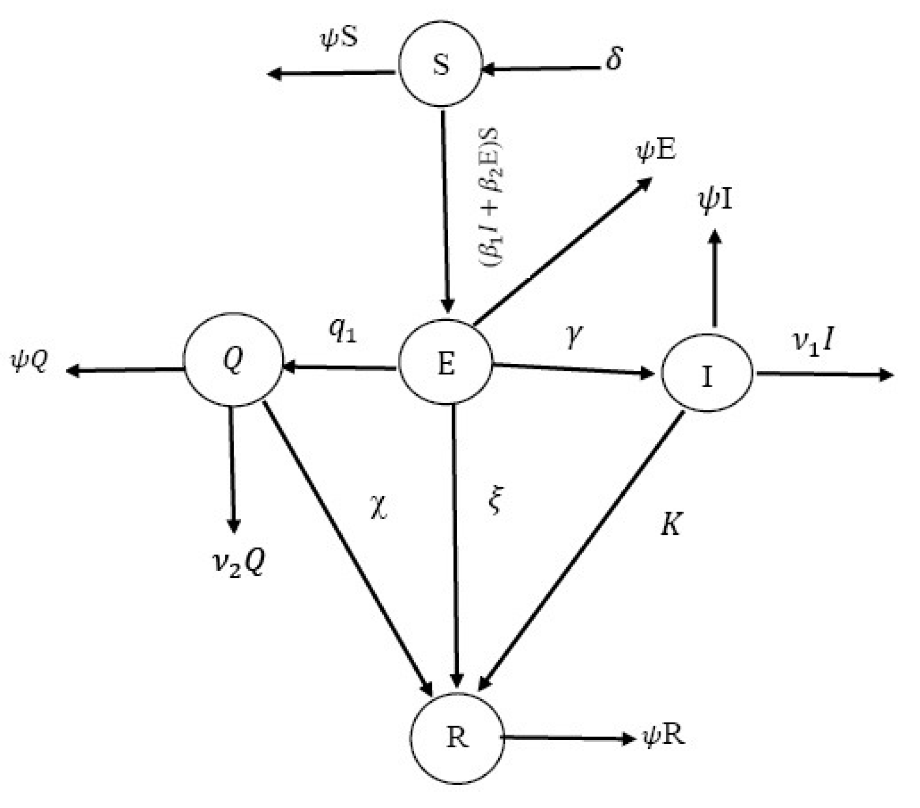
2.1. Some Concepts on the COVID-19 Model

The authors of [33] defined all of the biological functions and parameters required to build and formulate the COVID-19 model of a human population of size $N\left(t\right)=S\left(t\right)+E\left(t\right)+I\left(t\right)+Q\left(t\right)+R\left(t\right)$. In this model, susceptible individuals are denoted by $S\left(t\right)$, exposed individuals are $E\left(t\right)$, infected individuals are $I\left(t\right)$, quarantined persons are $Q\left(t\right)$, and individuals who have recovered from COVID-19 are $R\left(t\right)$. The dynamics of the spread of COVID-19 under the influences of these factors is described by a mathematical model in a form of the following nonlinear system of ODEs ($\forall t\ge 0$):

$$\begin{array}{cc}\hfill & \dot{S}\left(t\right)=-S\left(t\right)\left({\beta }_{1}I\left(t\right)+{\beta }_{2}E\left(t\right)\right)-\psi S\left(t\right)+\delta ,\hfill \\ & \dot{E}\left(t\right)=S\left(t\right)\left({\beta }_{1}I\left(t\right)+{\beta }_{2}E\left(t\right)\right)-\left(q_1+\xi +\gamma +\psi \right)E\left(t\right),\hfill \\ & \dot{I}\left(t\right)=\gamma E\left(t\right)-\left(K+\psi +{\nu }_1\right)I\left(t\right),\hfill \\ & \dot{Q}\left(t\right)=q_{1}E\left(t\right)-\left(\chi +\psi +{\nu }_2\right)Q\left(t\right),\hfill \\ & \dot{R}\left(t\right)=\xi E\left(t\right)+KI\left(t\right)+\chi Q\left(t\right)-\psi R\left(t\right).\hfill \end{array}$$

(1)

The parameters in this system are defined with the help of Figure 1 and [33]. We consider the initial sizes of $S\left(t\right),E\left(t\right),I\left(t\right),Q\left(t\right),$ and $R\left(t\right)$, as follows:

$$S\left(0\right)=S_0,E\left(0\right)=E_0,I\left(0\right)=I_0,Q\left(0\right)=Q_0,R\left(0\right)=R_0.$$

Figure 1. Flowchart describing the dynamics of propagation for the SEIQR model of COVID-19.

It is well known that the ODEs are commonly utilized to study anomalous natural occurrences as well as take into consideration the curve’s characteristics over a wide area, as a general case. The time delay, fractal features, etc. may finally be explained.

The authors of [33] considered the following cases to estimate ${\mathfrak{R}}_0$ (the reproductive number):

• If there is no COVID-19, the model ${\xi }_0=\left(S_{*}^0,E_{*}^0,I_{*}^0,Q_{*}^0,R_{*}^0\right)=(\delta /\psi ,0,0,0,0)$ is an equilibrium point.
• In general, the equilibrium takes the form ${\xi }_1=\left(S_{*}^1,E_{*}^1,I_{*}^1,Q_{*}^1,R_{*}^1\right)$, where

  $$S_{*}^1=\frac{\left(q_1+\xi +\gamma +\psi \right)\left(K+\psi +{\nu }_1\right)}{{\beta }_1\gamma +{\beta }_2\left(K+\psi +{\nu }_1\right)},E_{*}^1=\frac{\left(\delta -\psi S_{*}^1\right)\left(K+\psi +{\nu }_1\right)}{\left[{\beta }_1\gamma +{\beta }_2\left(K+\psi +{\nu }_1\right)\right]S_{*}^1},$$

  $$I_{*}^1=\frac{\gamma E_{*}^1}{K+\psi +{\nu }_1},Q_{*}^1=\frac{q_1{E}_{*}^1}{\chi +\psi +{\nu }_2},R_{*}^1=\frac{\xi E_{*}^1+K{I}_{*}^1+\chi Q_{*}^1}{\psi }.$$

Now, we can compute the corresponding Jacobian matrix of the nonlinear system of algebraic equations, which is obtained from the model (1) under the cases of ${\xi }_0$ and ${\xi }_1$, denoted by F and V, respectively. Thus, ${\mathfrak{R}}_0$ is defined as the average number of secondary infections produced when an infected person is introduced into a group of susceptible persons and is calculated by [33]:

$${\mathfrak{R}}_0=\rho \left(F{V}^{-1}\right)=\frac{\delta \left[{\beta }_2\left(K+\psi +{\nu }_1\right)+{\beta }_1\gamma \right]}{\left(\xi +\gamma +\psi +q_1\right)\left(K+\psi +{\nu }_1\right)},$$

(2)

where $\rho \left(P\right)$ is the spectral radius of a matrix P [34].

2.2. Non-Negative Solutions, Equilibrium Points and Stability

Theorem 1

([35]). For the proposed model (1), we have the following:

1.

${(S\left(t\right),E\left(t\right),I\left(t\right),Q\left(t\right),R\left(t\right))}^T$ is the unique solution of (1) and leftover in $R_{+}^5$.

2.

If ${\mathfrak{R}}_0<1$, then the disease free equilibrium point ${\xi }_0=(S_{*}^0,E_{*}^0,I_{*}^0,Q_{*}^0,R_{*}^0)$ is locally asymptotically stable (LAS).

3.

The endemic equilibrium point ${\xi }_1=(S_{*}^1,E_{*}^1,I_{*}^1,Q_{*}^1,R_{*}^1)$ is LAS iff ${\mathfrak{R}}_0>1$.

The proof of the three items in this theorem can be found in [35,36]. The given data here are utilized to estimate parameters using the least curve fitting method. Model (1) parameterizations are based on values from the literature. The actual data (from Wuhan, China) are accessible from 21 January 2020 throughto 28 January 2020, as shown in Table 1 in [37].

The primary contribution of this study is that we obtain a numerical framework for solving and performing essential comparisons on the coronavirus mathematical model. The number of patients and the expected number of infections with this disease due to the spread of infection and the number of infections after recovery can be predicted by solving this model. This information is extremely helpful for managing the disease’s health costs.

3. Numerical Implementation of the MSRM

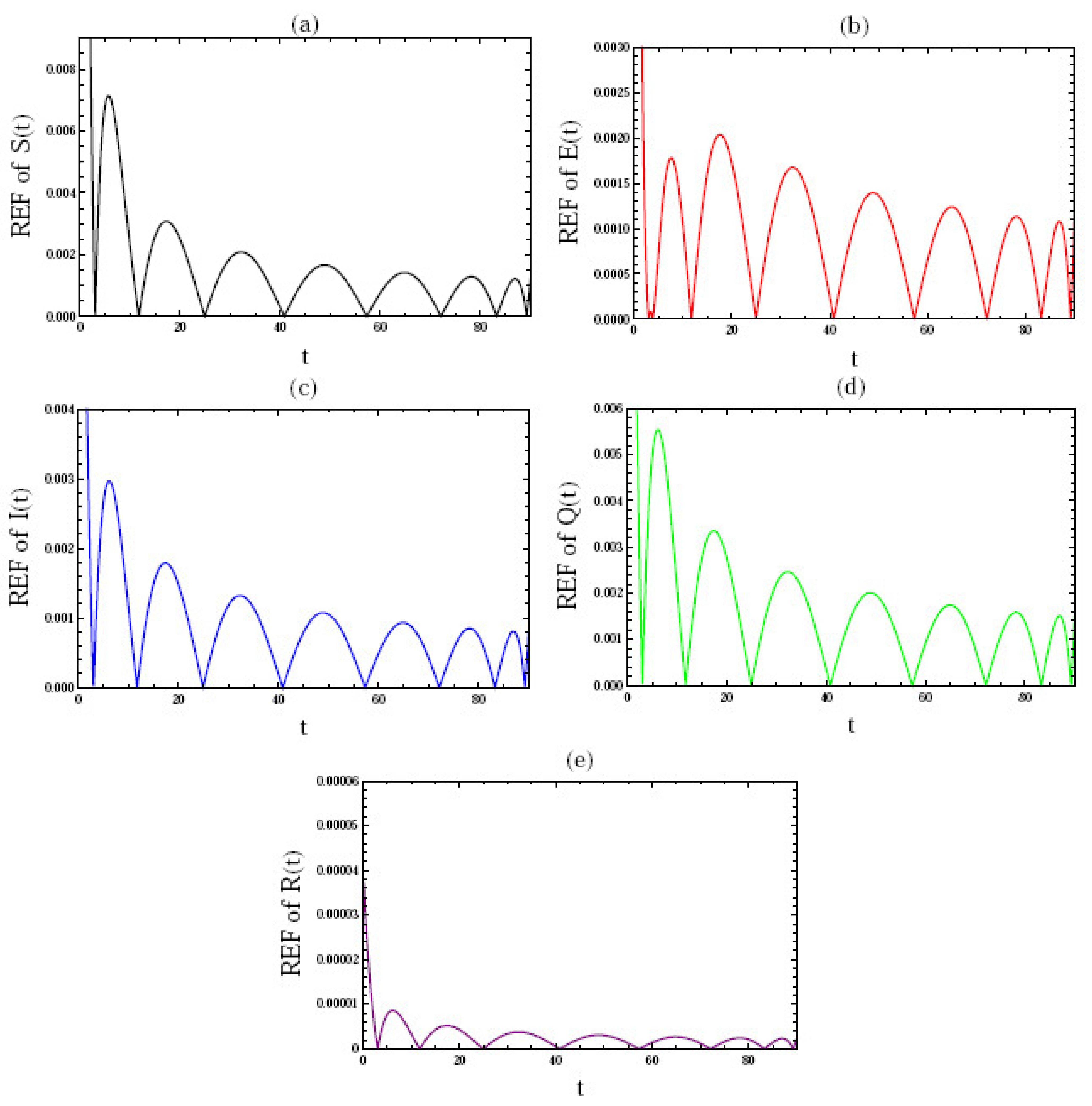
In this section, we apply the proposed method to get the analytical solution of the studied model numerically and greatly simplify it to a system of algebraic equations. This system is what we are going to study here, and it is formulated as follows:

$$\begin{array}{cc}\hfill & \dot{y_1}\left(t\right)=-y_1\left(t\right)\left({\beta }_1{y}_3\left(t\right)+{\beta }_2{y}_2\left(t\right)\right)-\psi y_1\left(t\right)+\delta ,\hfill \\ & \dot{y_2}\left(t\right)=y_1\left(t\right)\left({\beta }_1{y}_3\left(t\right)+{\beta }_2{y}_2\left(t\right)\right)-\left(q_1+\xi +\gamma +\psi \right)y_2\left(t\right),\hfill \\ & \dot{y_3}\left(t\right)=\gamma y_2\left(t\right)-\left(K+\psi +{\nu }_1\right)y_3\left(t\right),\hfill \\ & \dot{y_4}\left(t\right)=q_1{y}_2\left(t\right)-\left(\chi +\psi +{\nu }_2\right)y_4\left(t\right),\hfill \\ & \dot{y_5}\left(t\right)=\xi y_2\left(t\right)+K{y}_3\left(t\right)+\chi y_4\left(t\right)-\psi y_5\left(t\right).\hfill \end{array}$$

(3)

Without a loss of generality, we replace the components ($S\left(t\right),E\left(t\right),I\left(t\right),Q\left(t\right),R\left(t\right)$) of the model (1) with the notations ($y_1\left(t\right),y_2\left(t\right),y_3\left(t\right),y_4\left(t\right),y_5\left(t\right)$), respectively, and express the system (3) in the form

$$\dot{y}+Ay+\mathbf{N}\left(y\right)=0,$$

(4)

where $y\left(t\right)={\left[y_1\left(t\right),y_2\left(t\right),...,y_5\left(t\right)\right]}^T,$ and the $5\times 5$ matrix $A={\ell }_{i,j},i,j=1,2,3,4,5$ is given by:

$$A=\left(\begin{array}{ccccc}\psi & 0& 0& 0& 0\\ 0& q_1+\xi +\gamma +\psi & 0& 0& 0\\ 0& -\gamma & K+\psi +{\nu }_1& 0& 0\\ 0& -q_1& 0& \chi +\psi +{\nu }_2& 0\\ 0& -\xi & -K& -\chi & \psi \end{array}\right),$$

and the vector of nonlinear components of Equation (4), $\mathbf{N}\left(y\right)$, is given by:

$$\mathbf{N}\left(y\right)=\left(\begin{array}{c}-\delta +y_1\left(t\right)\left({\beta }_1{y}_3\left(t\right)+{\beta }_2{y}_2\left(t\right)\right)\\ -y_1\left(t\right)\left({\beta }_1{y}_3\left(t\right)+{\beta }_2{y}_2\left(t\right)\right)\\ 0\\ 0\\ 0\end{array}\right).$$

Now, we implement MSRM to solve Equation (4). The Chebyshev spectral approach is the foundation of the MSRM and uses the Chebyshev polynomials (ChPs) to estimate functions. The ChPs $T_k\left(z\right)$ of order k are formed as follows:

$$T_k\left(z\right)=cos\left(k{cos}^{-1}\left(z\right)\right),k\in \mathbb{N}.$$

(5)

Now, by using the interpolation concerning the Chebyshev polynomials, we can approximate the function $v\left(z\right)$ at $z=z_i$ by $v_m\left(z\right)$ that is defined by:

$$v_m\left(z\right)=\sum _{i=0}^m{v}_i{Ł}_i\left(z\right).$$

(6)

We use the Chebyshev–Gauss–Lobatto points (CGLPs) as collocation points $z_i$ from the following extreme points of $T_m\left(z\right)$:

$${\left\{z_i\right\}}_{i=0}^m=\left\{cos\left(\frac{\pi i}{m}\right),i=0,1,...,m\right\}.$$

(7)

This decision is made for the straightforward reason that the error is minimized in the Lagrangian interpolation if the interpolation points are taken to be the zeroes of the polynomial. The Lagrange polynomials ${Ł}_i\left(z\right),i=0,1,\dots ,m$, of order i based on the CGLPs are formulated as follows:

$${Ł}_i\left(z\right)=\frac{{(-1)}^{i+1}\left(1-z^2\right)T_i\left(z\right)}{{\hslash }_i{i}^2\left(z-z_i\right)},i=0,1,\dots ,m,$$

(8)

where ${\hslash }_0={\hslash }_m=2,{\hslash }_i=1$ for $i=1,2,\dots ,m-1$. Consequently, the first-order derivative of the approximate solution at the collocation nodes is calculated as follows:

$$\frac{dv\left(z\right)}{dz}=\sum _{k=0}^{m}v\left(z_k\right)\frac{{dŁ}_k\left(z_i\right)}{dz}=\sum _{k=0}^m{D}_{ik}v\left(z_k\right)=\mathbb{D}{V}_i,i=0,1,\dots ,m,$$

(9)

where $D_{ik}=\frac{{dŁ}_k\left(z_i\right)}{dz}$ is an $(m+1)\times (m+1)$ Chebyshev differentiation matrix (CDM) for $i,k=0,1,\dots ,m$. The entries of the CDM at $z_i$ is defined by [27,32]:

$$D_{ik}=\left\{\begin{array}{cc}\frac{{\hslash }_i{(-1)}^{k+i}}{{\hslash }_k\left(z_k-z_i\right)},\hfill & i\ne k,\hfill \\ -\frac{z_i}{2\left(1-z_i^2\right)},\hfill & (i=k)\ne 0,m,\hfill \\ \frac{2m^2+1}{6},\hfill & i,k=0,\hfill \\ -\frac{2m^2+1}{6},\hfill & i,k=m.\hfill \end{array}\right.$$

(10)

To solve Equation (4), firstly, we decompose the interval $I=[0,T]$ into n subintervals of length $\frac{T}{n}$, with each subdomain being $I_j=\left[t_{j-1},t_j\right]$ for $j=1,2,\dots ,n$ and having the property that

$$\bigcup _{j=1}^n\left[t_{j-1},t_j\right]=[0,T].$$

(11)

Using the following linear transformation, each subdomain $\left[t_{j-1},t_j\right]$ is converted to the interval $[-1,1]$, which is the domain of the CGLPs specified in Equation (7):

$$\widehat{t}=\frac{t_j-t_{j-1}}{2}z+\frac{t_{j-1}+t_j}{2}=\frac{T}{2n}z+\frac{t_{j-1}+t_j}{2},j=1,2,\dots ,n,$$

where $t_j-t_{j-1}=\frac{T}{n}.$

We approximate the derivatives in Equation (4) by using the CDM to lead a system of algebraic equations that we solve numerically for each subdomain, $I_j$, by using the Gauss–Seidel technique. We use $t_l^j$ as collocation points and $Y_s^j={\left[y_s\left(z_0^j\right),y_s\left(z_1^j\right),\cdots ,y_s\left(z_m^j\right)\right]}^T$ as an approximate solution in each subinterval. Substituting the CDM to approximate the first derivatives in Equation (4) yields the following system:

$$\left(\frac{2n}{T}\mathbb{D}+{\ell }_{s,s}I\right)Y_s^j+\sum _{\begin{array}{c}i=1\\ i\ne s\end{array}}^5{\ell }_{s,i}{Y}_i^j+N_s^j\left(Y\right)=0,s=1,2,3,4,5,$$

(12)

where

$$Y={\left[Y_1,Y_2,Y_3,Y_4,Y_5\right]}^T,N_s\left(Y\right)={\left[N_s\left(Y\left(z_0\right)\right),N_s\left(Y\left(z_1\right)\right),\dots ,N_s\left(Y\left(z_m\right)\right)\right]}^T.$$

In view of the Gauss–Seidel method for solving a system of algebraic equations, we can arrive at the following iteration formula of the system (12):

$$\left(\frac{2n}{T}\mathbb{D}+{\ell }_{s,s}I\right)Y_{s,p+1}^j=-\sum _{i=1}^{s-1}{\ell }_{s,i}{Y}_{i,p+1}^j-\sum _{i=s+1}^5{\ell }_{s,i}{Y}_{i,p}^j-N_{s,p,p+1}^j,s=1,2,3,4,5,$$

(13)

where $Y_{s,p+1}$ is the approximation of each $y_s$ at the ${(p+1)}^{\mathrm{th}}$ iteration and

$$N_{s,p,p+1}=N_s\left(Y_{1,p+1},Y_{2,p+1},\dots ,Y_{s-1,p+1},Y_{s,p},\dots ,Y_{5,p}\right).$$

We point out that data from the previous iteration are used to evaluate the nonlinear terms. As a result, the roughly approximate solution comes from

$$Y_{s,p+1}^j=A_s^{-1}{B}_s^j,s=1,2,3,4,5,$$

(14)

where

$$A_s=\frac{2p}{T}D+{\ell }_{r,r}I,B_s^j=-\sum _{i=1}^{s-1}{\ell }_{s,i}{Y}_{i,p+1}^j-\sum _{i=s+1}^5{\ell }_{s,i}{Y}_{i,p}^j-N_{s,p,p+1}^j.$$

The approximate solution of the system (4) on $[0,T]$ can be defined by

$$y_s=\bigcup _{j=1}^n{Y}_s^j\left(z^j\right).$$

4. Error Analysis

Here, we discuss the convergence analysis of the MSRM and estimate the error. Equation (12), can be written as

$$AY=B,$$

(15)

where

$$A=\left(\begin{array}{ccccc}\frac{2n}{T}\mathbb{D}+{\ell }_{1,1}I& {\ell }_{1,2}I& {\ell }_{1,3}I& {\ell }_{1,4}I& {\ell }_{1,5}I\\ {\ell }_{2,1}I& \frac{2n}{T}\mathbb{D}+{\ell }_{2,2}I& {\ell }_{2,3}I& {\ell }_{2,4}I& {\ell }_{2,5}I\\ {\ell }_{3,1}I& {\ell }_{3,2}I& \frac{2n}{T}\mathbb{D}+{\ell }_{3,3}I& {\ell }_{3,4}I& {\ell }_{3,5}I\\ {\ell }_{4,1}I& {\ell }_{4,2}I& {\ell }_{4,3}I& \frac{2n}{T}\mathbb{D}+{\ell }_{4,4}I& {\ell }_{4,5}I\\ {\ell }_{5,1}I& {\ell }_{5,2}I& {\ell }_{5,3}I& {\ell }_{5,4}I& \frac{2n}{T}\mathbb{D}+{\ell }_{5,5}I\end{array}\right),$$

$$Y^j=\left(\begin{array}{c}{Y}_1^j\\ Y_2^j\\ Y_3^j\\ Y_4^j\\ Y_5^j\end{array}\right)\mathrm{and}{B}^j=\left(\begin{array}{c}-N_1^j\\ -N_2^j\\ -N_3^j\\ -N_4^j\\ -N_5^j\end{array}\right).$$

Theorem 2.

Suppose that the coefficient matrix A is strictly diagonally dominant. Then, for any $Y^{\left(0\right)}\in {\mathbb{R}}^{\overline{n}}$, the sequence ${\left\{y^{\left(k\right)}\right\}}_{k=0}^{\infty }$ obtained from $Y=A^{-1}B$ converges to the unique solution $\overline{Y}$.

Proof. 

We demonstrate the diagonal dominance of matrix A above to prove the convergence. We take into account the norms of the matrices inside A since we are working with the block matrix A. For any $m\times n$ real matrix A, we can confirm the following norm equivalence:

$${\parallel A\parallel }_{max}\le {\parallel A\parallel }_2\le \sqrt{mn}{\parallel A\parallel }_{max},$$

where ${\parallel ·\parallel }_2$ is the spectral norm, and ${\parallel A\parallel }_{max}={max}_{\{i,j\}}\left|a_{i,j}\right|$. If $n>>1$, in Equation (15), then:

$$\frac{2n}{T}\mathbb{D}\gg {\ell }_{s,s}I,s=1,2,3,4,5.$$

This implies that

$${∥\frac{2n}{T}\mathbb{D}+{\ell }_{s,s}I∥}_{max}\approx \left|\frac{2n}{T}\lambda \right|,$$

where $\lambda$ is a nonzero constant that is independent of $\frac{n}{T}$. Similarly,

$$\sum _{j=1,j\ne s}^5{∥{\ell }_{s,j}I∥}_{max}=\sum _{j=1,j\ne s}^5\left|{\ell }_{s,j}\right|.$$

Thus, for n sufficiently large, we have

$${∥\frac{2n}{T}\mathbb{D}+{\ell }_{s,s}I∥}_{max}\approx \left|\frac{2n}{T}\lambda \right|\ge \sum _{j=1,j\ne s}^5\left|{\ell }_{s,j}\right|=\sum _{j=1,j\ne s}^5∥{\ell }_{s,j}I∥.$$

Therefore, the block matrix A is diagonally dominant. Hence, the method converges. □

Theorem 3

([38]). Suppose that $y_s\left(t\right)\in C^{m+1}[0,T]$ interpolated by a polynomial $Y_s\left(t\right)$ of degree $\le m$ at $m+1$ distinct points $z_0,z_1,\dots ,z_m\in \left[t_{j-1},t_j\right]$ with the property (11).

Let $z_i$ be the nodes that are chosen as the Gauss–Lobatto points (7), then the resulting error from the polynomial interpolation in $[0,T]$ in each subdomain is estimated by

$$E\left(t\right)=\left|y_s\left(t\right)-Y_s\left(t\right)\right|\le {\left(\frac{T}{2}\right)}^{m+1}{\left(\frac{1}{n}\right)}^m\frac{\theta }{2^{m-1}(m+1)!},$$

where $\theta \ne 0$.

For $n>>1$, because of the factor ${\left(\frac{1}{n}\right)}^m<<1$, the error in the case of multidomain is much smaller than the single-domain case, $n=1$.

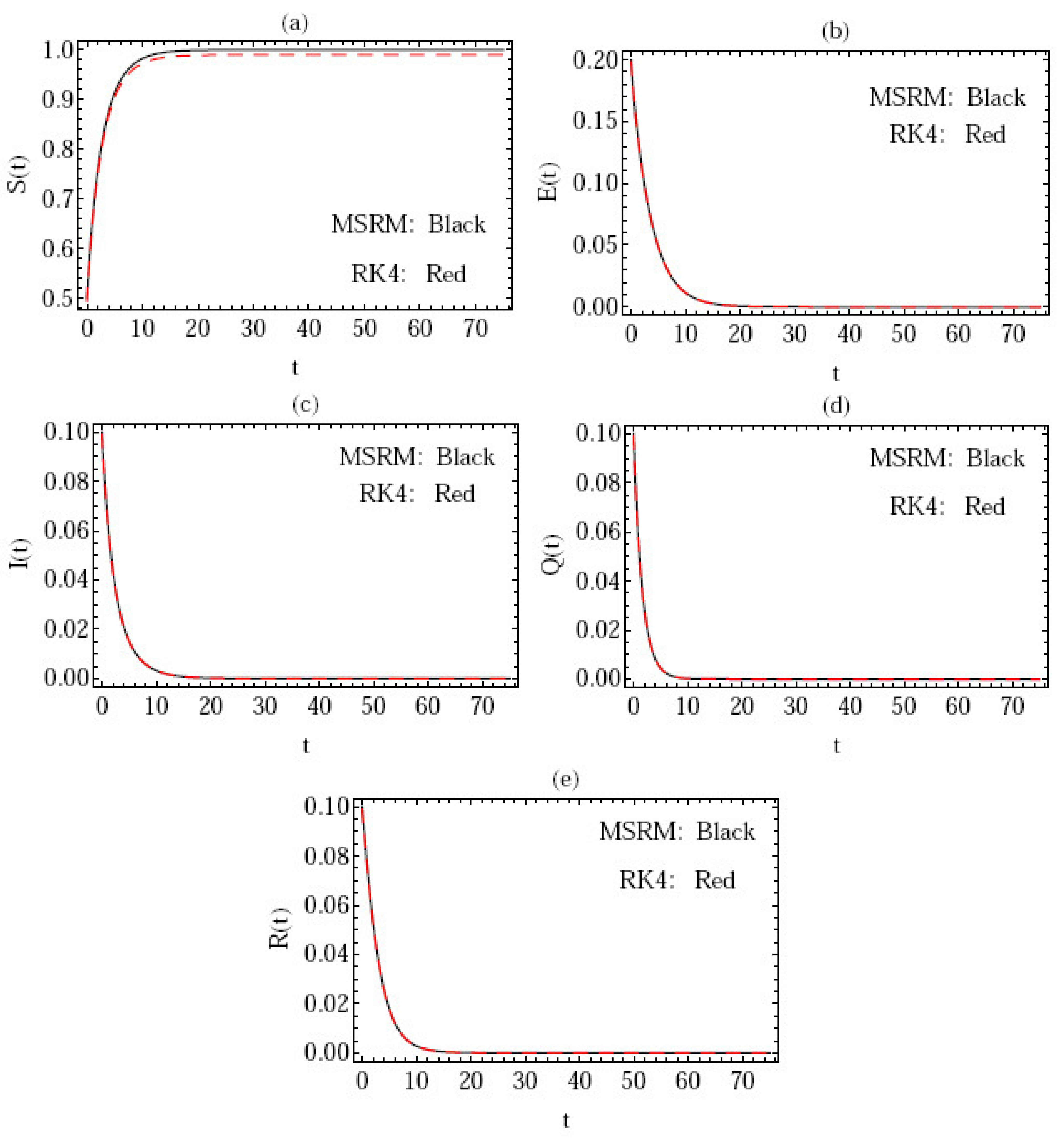
5. Numerical Simulation

We show some numerical simulations in this section of the model (1) with various values of $\delta ,{\beta }_1,{\beta }_2,\psi ,q_1,\xi ,{\nu }_1,{\nu }_2,\gamma ,K,\chi ,$ and the initial conditions $S_0,E_0,I_0,Q_0,R_0.$ Figure 2, Figure 3, Figure 4, Figure 5 and Figure 6 illustrate the numerical results for the examined system by implementing the suggested method. All numerical results were obtained with Mathematica.

Figure 2. The solution via different values of m.

Figure 3. Variations in the behavior of the approximation in the starting values.

Figure 4. The approximate solution against distinct values of $q_1$.

Figure 5. The REF of the solutions.

Figure 6. The approximate solution given by the MSRM and RK4 methods.

• Figure 2 shows how the approximate solution behaves for various approximation orders, $m=4$ (Figure 2a) and $m=6$ (Figure 2b), in the domain ($0,25$) with $S_0=0.5,E_0=0.2,I_0=Q_0=R_0=0.1$ and the parameters $\delta =0.5,{\beta }_1=1.05,{\beta }_2=0.005,\psi =0.5,q_1=0.001,\xi =0.00398,{\nu }_1=0.0047876,{\nu }_2=0.000001231,\gamma =0.085432,K=0.09871,\chi =0.1243.$ In this case, ${\mathfrak{R}}_0=0.130112<1$, and Theorem 1 also allows us to observe that the disease-free equilibrium point ${\xi }_0$ is LAS.
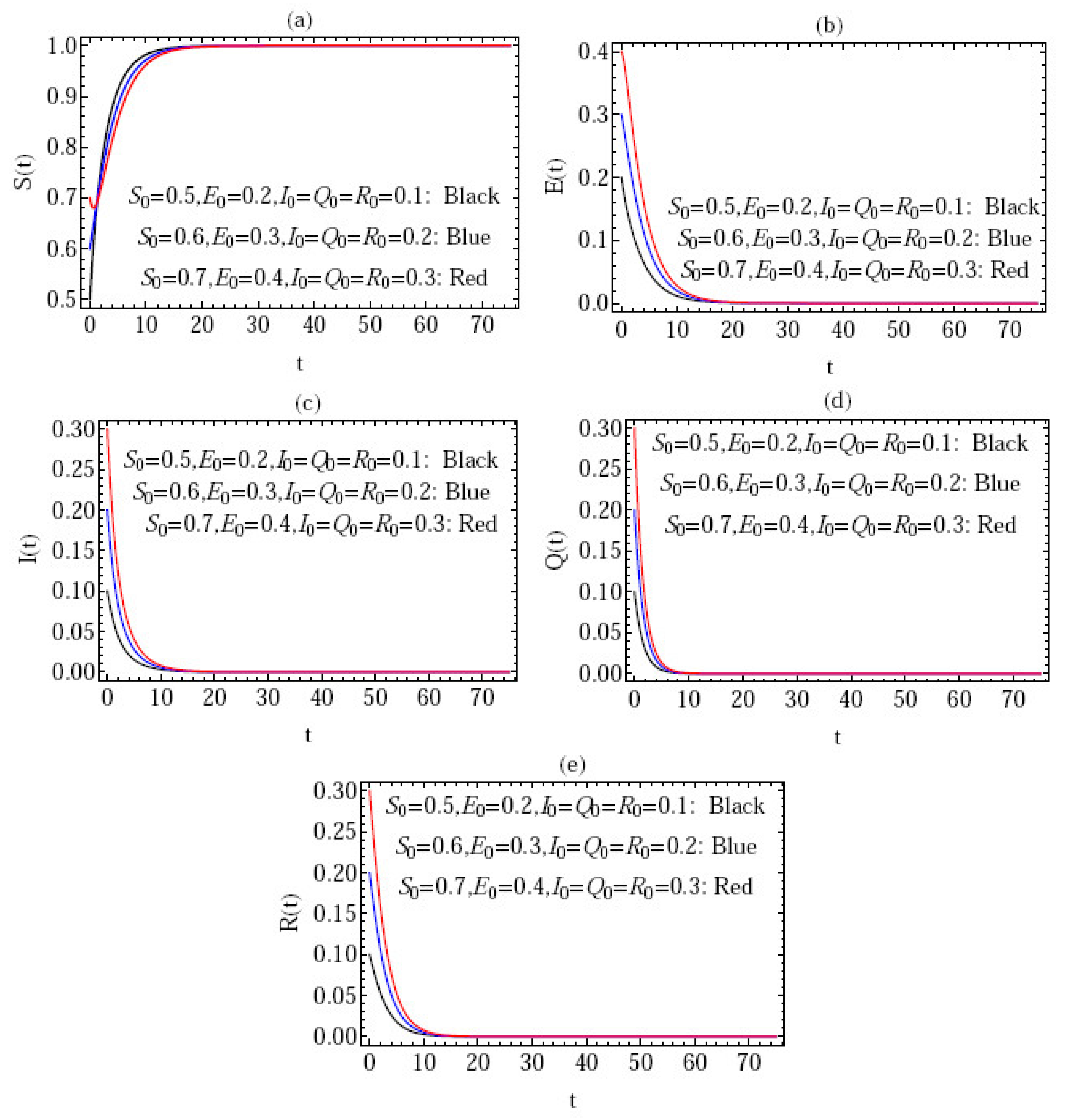
• Figure 3 gives the behavior of the approximate solution under the distinct initial solution with $m=6$ in the interval ($0,75$), and the parameters $\delta =0.5,{\beta }_1=1.05,{\beta }_2=0.005,\psi =0.5,q_1=0.001,\xi =0.00398,{\nu }_1=0.0047876,{\nu }_2=0.000001231,\gamma =0.085432,K=0.09871,\chi =0.1243$; where $S\left(t\right),E\left(t\right),I\left(t\right),Q\left(t\right),R\left(t\right)$ are plotted in Figure 3a–e, respectively. Here, we give the following three cases:

  i.

  $S_0=0.5,E_0=0.2,I_0=Q_0=R_0=0.1$;

  ii.

  $S_0=0.6,E_0=0.3,I_0=Q_0=R_0=0.2$;

  iii.

  $S_0=0.7,E_0=0.4,I_0=Q_0=R_0=0.3$.

  In the above three cases, we can confirm that the condition of stability is satisfied, i.e., ${\mathfrak{R}}_0<1$.
• The approximate solution via distinct values of $q_1=0.1,0.5,0.9$ with $m=6$ in the interval ($0,75$) with the same initial values as in Figure 2 is presented in Figure 4, and in these cases, we find that ${\mathfrak{R}}_0<1$.
• To estimate the accuracy of the proposed scheme, we give the residual error function (REF) in Figure 5 with $m=6$ and the same parameters and initial conditions as shown in Figure 2.
• The approximate solutions provided by the MSRM and RK4 methods (at $h=0.05$) are compared in Figure 6 with the same parameters and initial conditions as in Figure 2. This graphic demonstrates that the theoretical stability findings found in the previous section are accurate.
  As shown in Figure 2 through Figure 6, the approximate solution is affected by the values of $m,q_1$, the initial conditions, and the added parameters $\delta ,{\beta }_1,{\beta }_2,\psi ,\xi ,{\nu }_1,$${\nu }_2,\gamma ,K,\chi$. This shows that the suggested technique can be effectively applied to solve the presented model.

It appears that the bulk of the population will recover from COVID-19, as shown in Figure 3, Figure 4, Figure 5 and Figure 6, since the recovered population expands significantly in Figure 3e. As shown in Figure 3b–d, we can also verify and corroborate a considerable decline in the populations of infected and exposed people. This implies that the vast majority of the populace will recover, which reduces the number of deaths brought on by COVID-19. The fact that the disease has behaved as expected has been confirmed, and this is simulated by the model. Additionally, understanding the behavior of all the model’s constituent parts is the basis for obtaining a sound physical interpretation of the obtained numerical results.

The findings show that as individuals come into contact with exposed or infected persons, their susceptibility will decline at consistent rates, resulting in bigger numbers of exposed individuals and drops and increases when more people exposed to COVID-19 get the infection. Likewise, as a proportion of recovered people pass away from natural causes, fewer people are exposed, infected, or placed in quarantine. Additionally, there are fluctuations in the proportion of those quarantined to people who have been exposed overall.

6. Conclusions

The Chebyshev spectral approach and the MSRM attributes were used to solve the model under study. The upper bound of the error was given and explored together with the examination of the convergence of the numerical solution. The answers to the researched problem’s solutions demonstrate how well the suggested method works for studying this subject. We also showed that the errors will decrease if we use additional terms from the series of the approximation solution. To determine whether the presented procedure is appropriate for such models, numerical solutions were calculated with different values of variables and parameters, along with the REF. We may infer the following points in view of the numerical simulation:

• The suggested approach is efficient and reliable.
• The approach has the capacity to apply a limited number of series solution terms to produce precise results.
• There are several benefits to using this approach to solve this kind of problem.

Additionally, we may advise that by increasing the public’s knowledge and encouraging people to follow government directives, the amount of susceptible people will decrease, and the number of infected people in the population will increase which, in turn, will significantly lessen the severity of infection. Finally, since we can only evaluate the solution at the nodes of the supplied interval and it is not unconditionally stable, the finite difference approach has some shortcomings. This is similar to how some numerical methods have some restrictions. Future tasks include addressing the same problem using various approaches, such as the finite element method, the finite volume method, and others; controlling the results optimally; and conducting in-depth research on the COVID-19 model’s theoretical underpinnings.

References

- Ahmed, I.; Modu, G.U.; Yusuf, A.; Kumam, P.; Yusuf, I. A mathematical model of Coronavirus Disease (COVID-19) containing asymptomatic and symptomatic classes. Results Phys. 2021, 21, 103776. [Google Scholar] [CrossRef]
- Sen, M.D.; Ibeas, A.; Agarwal, R.P. On confinement and quarantine concerns on an SEIAR epidemic model with simulated parameterizations for the COVID-19 pandemic. Symmetry 2020, 12, 1646. [Google Scholar] [CrossRef]
- Srinivasa, K.; Baskonus, H.M.; Sanchez, Y.G. Numerical solutions of the mathematical models on the digestive system and COVID-19 pandemic by Hermite wavelet technique. Symmetry 2021, 13, 2428. [Google Scholar] [CrossRef]
- World Health Organization. Report of the WHO—China Joint Mission on Coronavirus Disease: 2019 (COVID-19); World Health Organization: Geneva, Switzerland, 2020. [Google Scholar]
- Agarwal, P.; Agarwal, R.P.; Ruzhansky, M. Special Functions and Analysis of Differential Equations; Chapman and Hall/CRC: Boca Raton, FL, USA, 2020. [Google Scholar]
- Basti, B.; Hammami, N.; Berrabah, I.; Nouioua, F.; Djemiat, R.; Benhamidouche, N. Stability analysis and existence of solutions for a modified SIRD model of COVID-19 with fractional derivatives. Symmetry 2021, 13, 1431. [Google Scholar] [CrossRef]
- Abd-Elhameed, W.M. Novel expressions for the derivatives of sixth kind Chebyshev polynomials: Spectral solution of the non-linear one-dimensional Burgers’ equation. Fractal Fract. 2021, 5, 53. [Google Scholar] [CrossRef]
- Sweilam, N.H.; Khader, M.M.; Adel, M. On the fundamental equations for modeling neuronal dynamics. J. Adv. Res. 2014, 5, 253–259. [Google Scholar] [CrossRef]
- Khader, M.M.; Sweilam, N.H.; Mahdy, A.M.S.; Moniem, N.K.A. Numerical simulation for the fractional SIRC model and influenza A. Appl. Math. Inf. Sci. 2014, 8, 1029–1036. [Google Scholar] [CrossRef]
- Aslan, M.F.; Sabanci, K.; Ropelewska, E. A new approach to COVID-19 detection: An ANN proposal optimized through tree-seed algorithm. Symmetry 2022, 14, 1310. [Google Scholar] [CrossRef]
- Anderson, R.M.; May, R.M. Helminth infections of humans: Mathematical models, population dynamics. and control. Adv. Parasitol. 1985, 24, 1–101. [Google Scholar]
- Meng, X.; Zhao, S.; Feng, T.; Zhang, T. Dynamics of a novel nonlinear stochastic SIS epidemic model with the double epidemic hypothesis. J. Math. Anal. Appl. 2016, 433, 227–242. [Google Scholar] [CrossRef]
- Kabir, K.A.; Kuga, K.; Tanimoto, J. Analysis of SIR epidemic model with information spreading of awareness. Chaos Solitons Fract. 2019, 119, 118–125. [Google Scholar] [CrossRef]
- Dokuyucu, M.A.; Celik, E.; Bulut, H.; Baskonus, H.M. Cancer treatment model with the Caputo-Fabrizio fractional derivative. Eur. Phys. J. Plus 2018, 133, 92. [Google Scholar] [CrossRef]
- Gunwehan, H.; Kaabar, K.A.K.; Celik, E. Novel Analytical and Approximate-Analytical Methods for Solving the Nonlinear Fractional Smoking Mathematical Model. Sigma J. Eng. Nat. Sci. 2022. [Google Scholar] [CrossRef]
- Adel, M.; Sweilam, N.H.; Khader, M.M.; Ahmed, S.M.; Ahmad, H.; Botmart, T. Numerical simulation using the non-standard weighted average FDM for 2Dim variable-order Cable equation. Results Phys. 2022, 39, 105682. [Google Scholar] [CrossRef]
- Dokuyucu, M.A.; Celik, E. Analyzing a novel coronavirus model (COVID-19) in the sense of Caputo-Fabrizio fractional operator. Appl. Comput. Math. 2021, 20, 49–69. [Google Scholar]
- Agarwal, P.; Nieto, J.J.; Ruzhansky, M.; Torres, D.F.M. Analysis of Infectious Disease Problems (COVID-19) and their Global Impact; Springer: Singapore, 2021. [Google Scholar]
- Batiha, I.M.; Obeidat, A.; Alshorm, S.; Alotaibi, A.; Alsubaie, H.; Momani, S.; Albdareen, M.; Zouidi, F.; Jahanshahi, S.M.E.H. A numerical confirmation of a fractional-order COVID-19 Model’s efficiency. Symmetry 2022, 14, 2583. [Google Scholar] [CrossRef]
- Abuasbeh, K.; Shafqat, R.; Alsinai, A.; Awadalla, M. Analysis of the mathematical modeling of COVID-19 by using mild solution with delay Caputo operator. Symmetry 2023, 15, 286. [Google Scholar] [CrossRef]
- Butt, A.I.K.; Imran, M.; Batool, S.; Nuwairan, M.A. Theoretical analysis of a COVID-19 CF-fractional model to optimally control the spread of pandemic. Symmetry 2023, 15, 380. [Google Scholar] [CrossRef]
- Khader, M.M.; Adel, M. Chebyshev wavelet procedure for solving FLDEs. Acta Appl. Math. 2018, 158, 1–10. [Google Scholar] [CrossRef]
- Chowdhury, M.S.H.; Hashim, I.; Momani, S. The multistage homotopy-perturbation method: A powerful scheme for handling the Lorenz system. Chaos Solitons Fractals 2009, 40, 1929–1937. [Google Scholar] [CrossRef]
- Motsa, S.S.; Dlamini, P.; Khumalo, M. A new multistage spectral relaxation method for solving chaotic initial value systems. Nonlinear Dyn. 2013, 72, 265–283. [Google Scholar] [CrossRef]
- Motsa, S.S.; Dlamini, P.G.; Khumalo, M. Solving hyperchaotic systems using the spectral relaxation method. Abstr. Appl. Anal. 2012, 2012, 203461. [Google Scholar] [CrossRef]
- Khan, M.S.; Khan, M.I. A novel numerical algorithm based on Galerkin-Petrov time-discretization method for solving chaotic nonlinear dynamical systems. Nonlinear Dyn. 2018, 91, 1555–1569. [Google Scholar] [CrossRef]
- Canuto, C.; Hussaini, M.Y.; Quarteroni, A.; Zang, T.A. Spectral Methods in Fluid Dynamics; Springer: New York, NY, USA, 1988. [Google Scholar]
- Kouagou, J.N.; Dlamini, P.G.; Simelane, S.M. On the multi-domain compact finite difference relaxation method for high dimensional chaos: The nine-dimensional Lorenz system. Alex. Eng. J. 2020, 59, 2617–2625. [Google Scholar] [CrossRef]
- Ibrahim, Y.; Khader, M.M.; Megahed, A.; Abdelsalam, F.; Adel, M. An efficient numerical simulation for a fractional COVID-19 model by using the GRK4M together with and the fractional FDM. Fractal Fract. 2022, 12, 304. [Google Scholar] [CrossRef]
- Abd-Elhameed, W.M.; Youssri, Y.H. Sixth-kind Chebyshev spectral approach for solving fractional differential equations. Int. J. Nonlinear Sci. Numer. Simul. 2019, 20, 191–203. [Google Scholar] [CrossRef]
- Abd-Elhameed, W.M. New Galerkin operational matrix of derivatives for solving Lane-Emden singular-type equations. Eur. Phys. J. Plus 2015, 130, 52. [Google Scholar] [CrossRef]
- Trefethen, L.N. Spectral Methods in MATLAB; SIAM: Philadelphia, PA, USA, 2000. [Google Scholar]
- Rafiq, M.; Macias-Diaz, J.E.; Raza, A.; Ahmed, N. Design of a nonlinear model for the propagation of COVID-19 and its efficient nonstandard computational implementation. Appl. Math. Model. 2021, 89, 1835–1846. [Google Scholar] [CrossRef]
- Diekmann, O.; Heesterbeek, J.A.P.; Metz, J.A. On the definition and the computation of the basic reproduction ratio R0 in models for infectious diseases in heterogeneous populations. J. Math. Biol. 1990, 14, 365–382. [Google Scholar]
- Khader, M.M.; Adel, M. Modeling and numerical simulation for covering the fractional COVID-19 model using spectral collocation-optimization algorithm. Fractal Fract. 2022, 6, 363. [Google Scholar] [CrossRef]
- Kumar, R.; Kumar, S. A new fractional modeling on Susceptible-Infected-Recovered equations with constant vaccination rate. Nonlinear Eng. 2014, 3, 11–16. [Google Scholar] [CrossRef]
- Khan, M.A.; Atangana, A. Modeling the dynamics of novel coronavirus (2019-nCoV) with fractional derivative. Alex. Eng. J. 2020, 56, 2379–2389. [Google Scholar] [CrossRef]
- Dlamini, P.; Simelane, S. An efficient spectral method-based algorithm for solving a high-dimensional chaotic Lorenz system. J. Appl. Comput. Mech. 2021, 7, 225–234. [Google Scholar]
Disclaimer/Publisher’s Note: The statements, opinions and data contained in all publications are solely those of the individual author(s) and contributor(s) and not of MDPI and/or the editor(s). MDPI and/or the editor(s) disclaim responsibility for any injury to people or property resulting from any ideas, methods, instructions or products referred to in the content. |
© 2023 by the authors. Licensee MDPI, Basel, Switzerland. This article is an open access article distributed under the terms and conditions of the Creative Commons Attribution (CC BY) license (https://creativecommons.org/licenses/by/4.0/).