

A Malware Detection Approach Based on Deep Learning and Memory Forensics

 , ,
, ,
Abstract
:1. Introduction
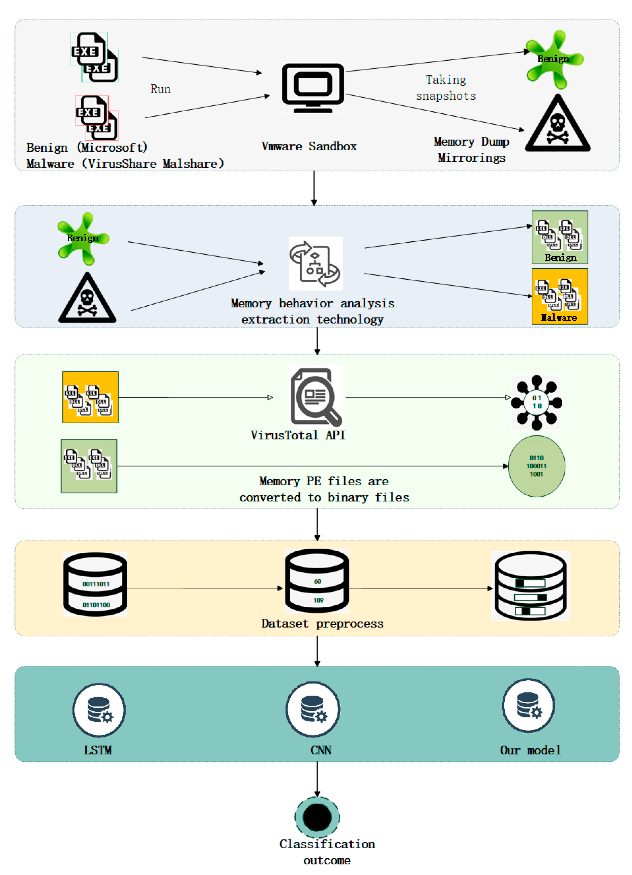
- This paper builds a portable executable (PE) file dataset in memory, which extracts more malicious memory samples in the process. This paper first collects static PE files from the well-known malicious sample libraries VirusShare and MalShare, which are widely used by researchers and have high persuasiveness. Then, this paper downloads the common software from the official Microsoft platform. Finally, it executes the static samples in running virtual machines and extracts the dynamic samples to create our dataset;
- We build a model based on the neural network (CNN), and use the model to train memory segments to achieve accurate detection of malicious code;
- We give an example of fileless malware attack in the paper. Since the dynamic file dataset is constructed, it has good detection performance for “no file” attacks and malicious samples that can only be detected in dynamic files.
2. Related Work
2.1. Memory Forensics
2.2. Malware Detection
3. Memory PE File Extraction Technology
3.1. Memory Analysis
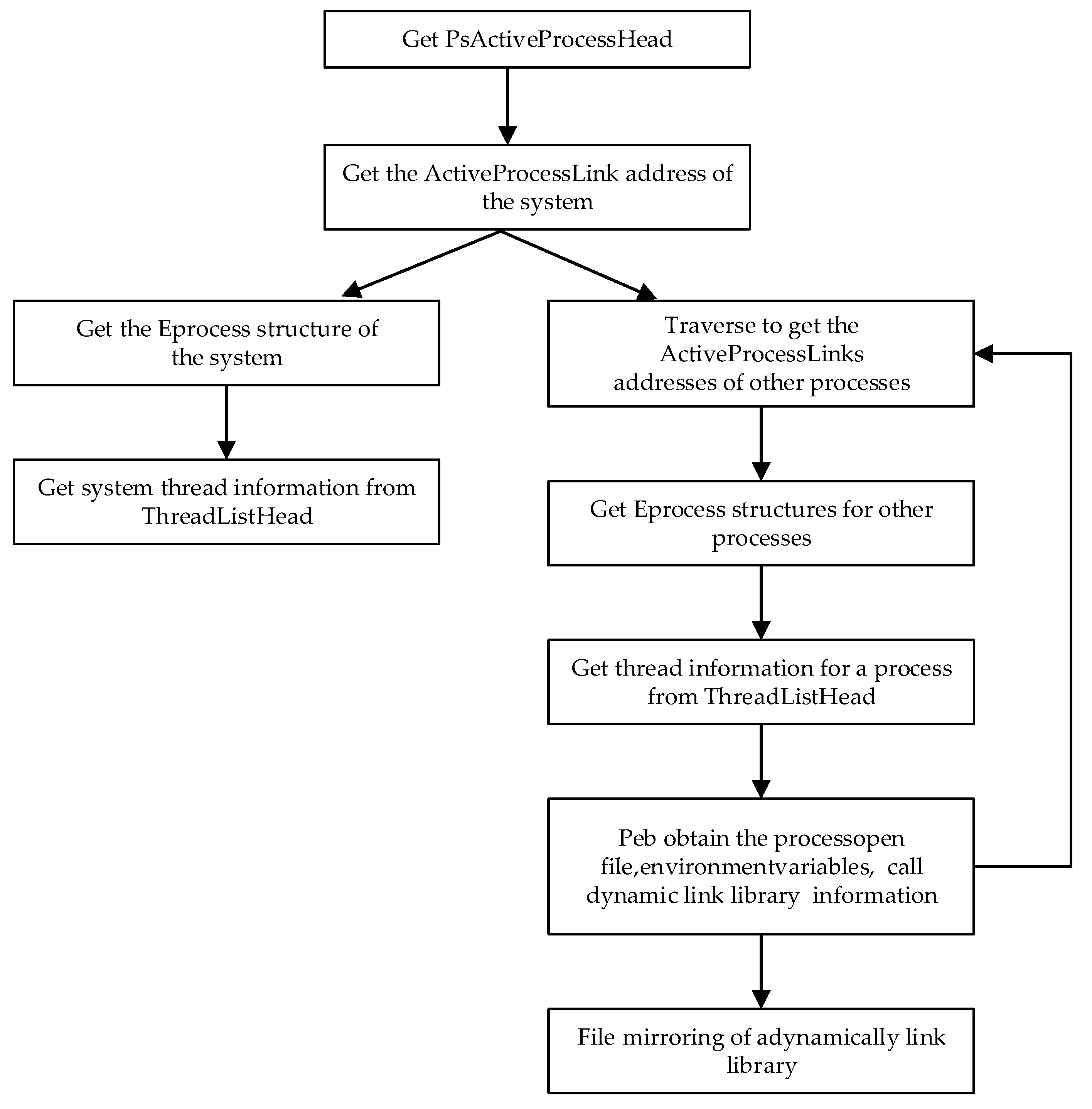
- The CR3 content and address translation mode are determined according to the KPCR structure. The brief process is as follows: KPCR structure -> KPCRB member -> ProcessorState member -> SpecialRegister member -> CR3 register;
- PsActiveProcessHead is determined according to the KPCR structure, and the process is as follows: KPCR structure -> KdVersionBlock -> PsActiveProcessHead;
- To obtain information about the processes, “PsActiveProcessHead” and “ActiveProcessLinks” are used to identify the system processes; thus, a two-way linked list can be traversed, and all activities of the process can be enumerated.
3.2. Memory Forensics
- Firstly, locate the page directory table (line1) by the value of the page directory base address. Read the page directory entry (PDE) in the page directory table and determine whether the directory entry is empty. If the directory entry is not empty, then mark the page directory entry as D. If D&1 equals 1, then mark the value of D&0xFFFFF000 as the physical address of the page table specified by the directory entry as T. If D&1 not equals 1, proceed to the next non-empty page directory entry;
- Secondly, read the first non-empty page entry of the page table. Page table entries are marked T, and if T&1 equals 1, mark the value of T&0xFFFFF000 as T as the physical address of the physical page specified by the page entry. Locate the physical address in the memory image, read the contents of the physical memory page, and dump the PE data of a single memory into the specified file in the memory image through the specified physical address. The algorithm (from lines 2 to 15) traverses the entire page table of contents.
| Algorithm 1 Process space dump algorithm. |
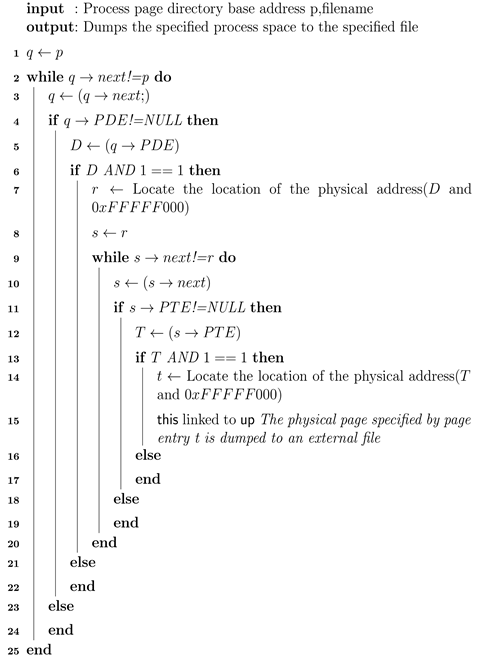 |
4. The Approach
4.1. Gathering Memory Data
4.2. Dataset Preprocessing
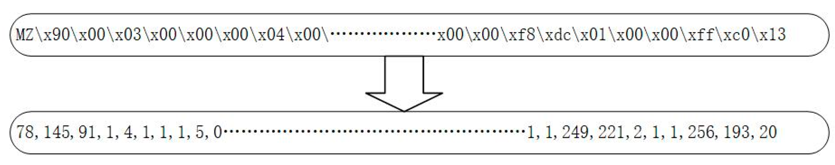
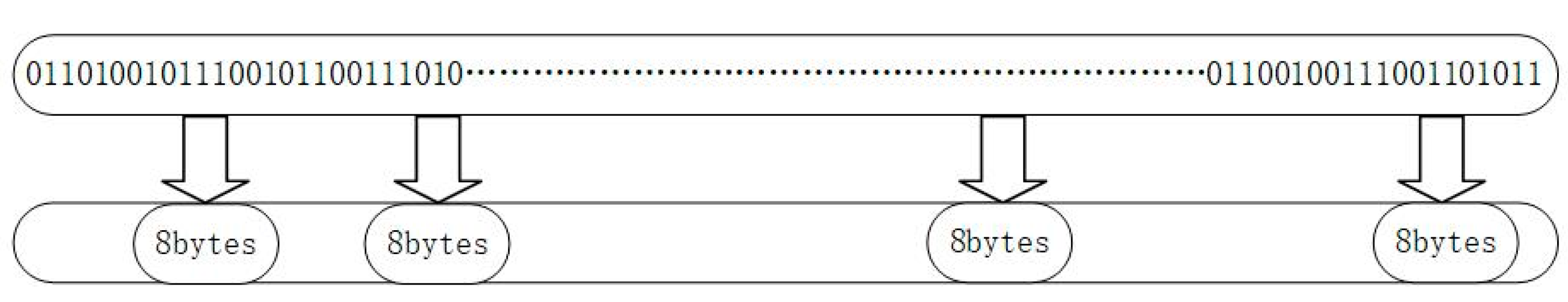
4.2.1. Data Type Conversion
4.2.2. Segment Selection
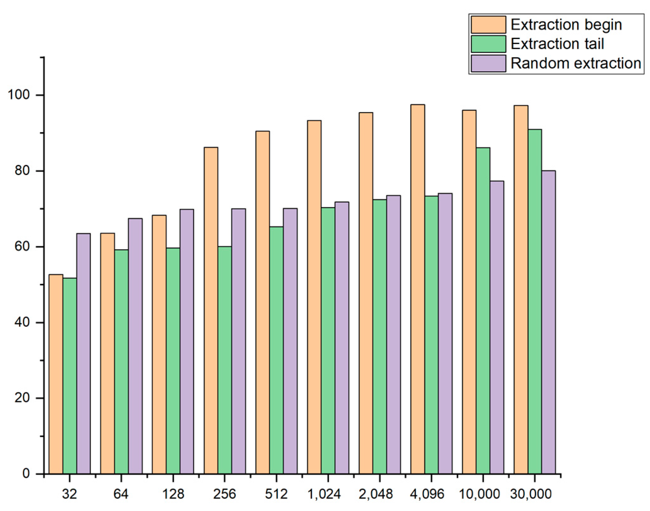
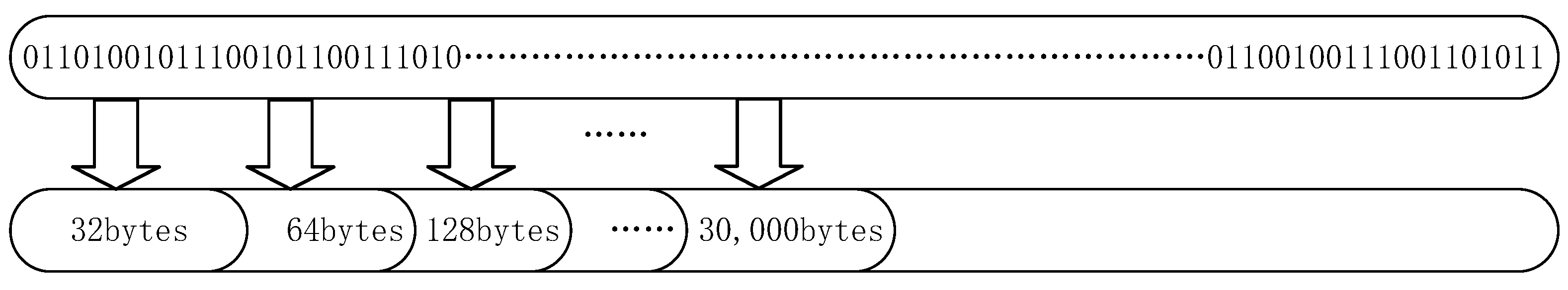
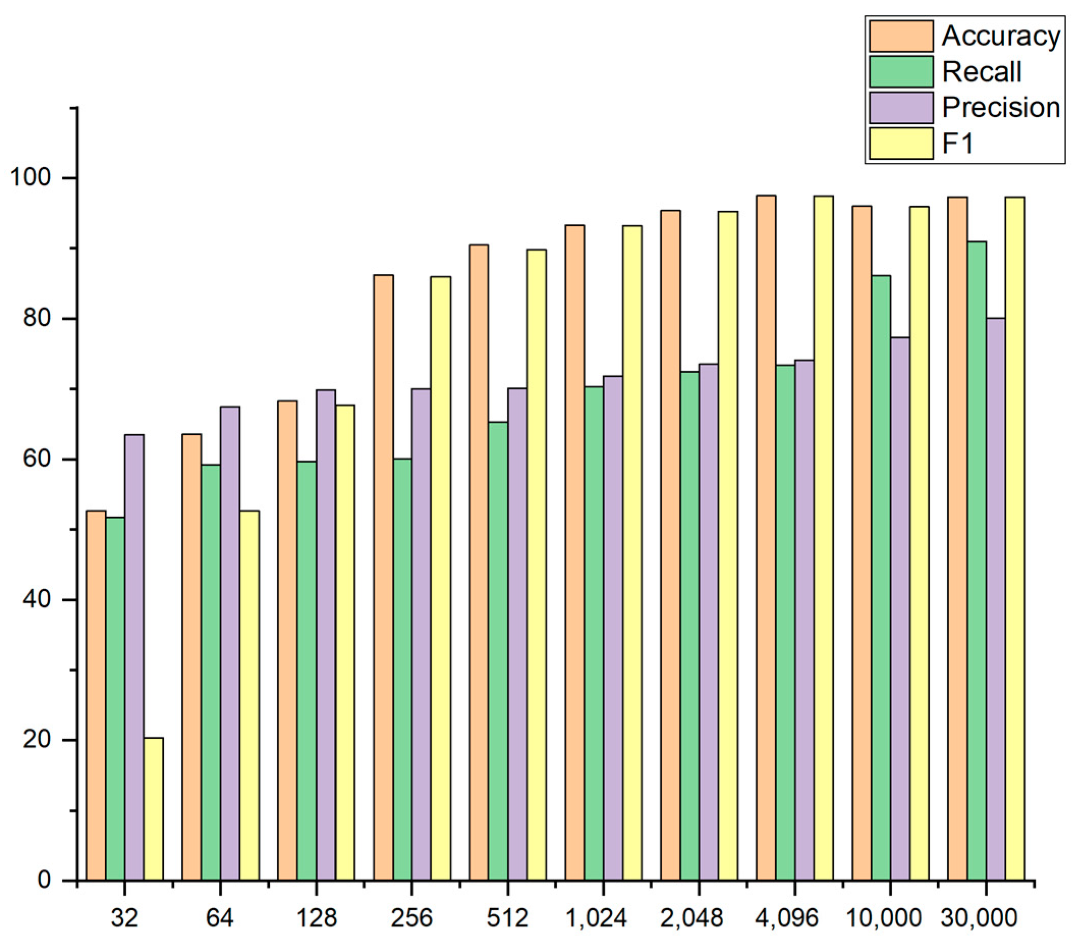
- As is shown in Figure 4, the sample header is selected for fragmentation, and the lengths of the header for the fragmentation are 32, 64, 128, 256, 512, 1024, 2048, 4096, 10,000, and 30,000 bytes. The effect of taking different lengths of the sample fragments on the model’s accuracy is observed through experiments. Additionally, the method of sample fragment training can also improve the detection efficiency of the model and significantly reduce the time taken for sample detection;
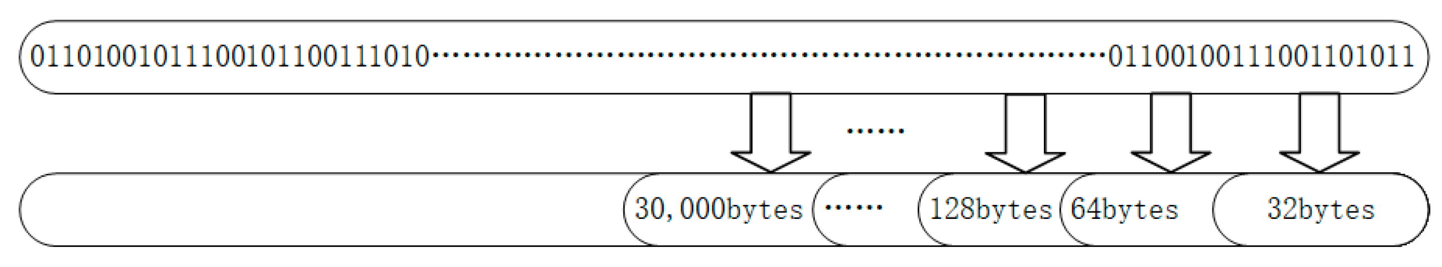
- As is shown in Figure 5, the tail of the sample is selected for the fragmentation such that the influence of the different positions of the fragment on the training accuracy can be judged. The tail is chosen to extract the sample fragment, and the extracted length is the same as the length extracted from the header, so the effect of the different positions can be better performed;
- As is shown in Figure 6, samples for the fragmentation are selected randomly. To better reflect the influence of the different locations on the experimental results, samples with the same fragment length but other locations are randomly extracted for each sample.
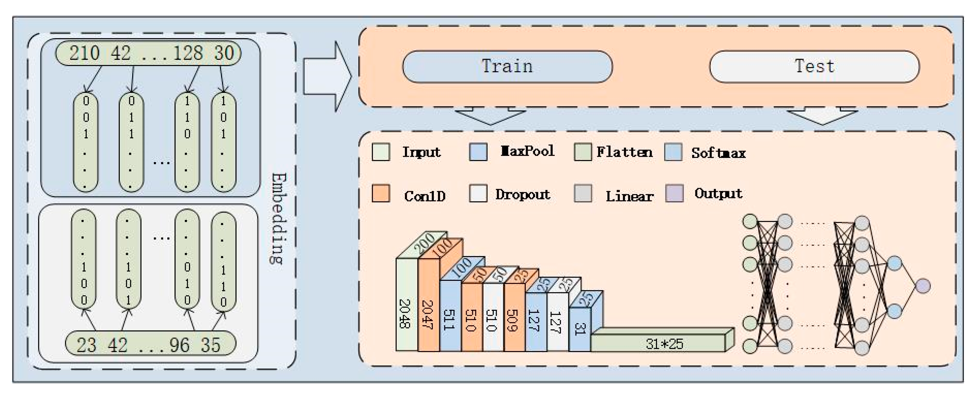
4.3. Our Model
4.4. Neural Network Algorithm
5. Experimental Overview
5.1. Operating Environment and Datasets
5.2. Evaluation Metrics
5.3. Datasets Parameter Optimization
5.4. Sample Fragments of Different Lengths
5.5. Sample Fragments of Different Lengths
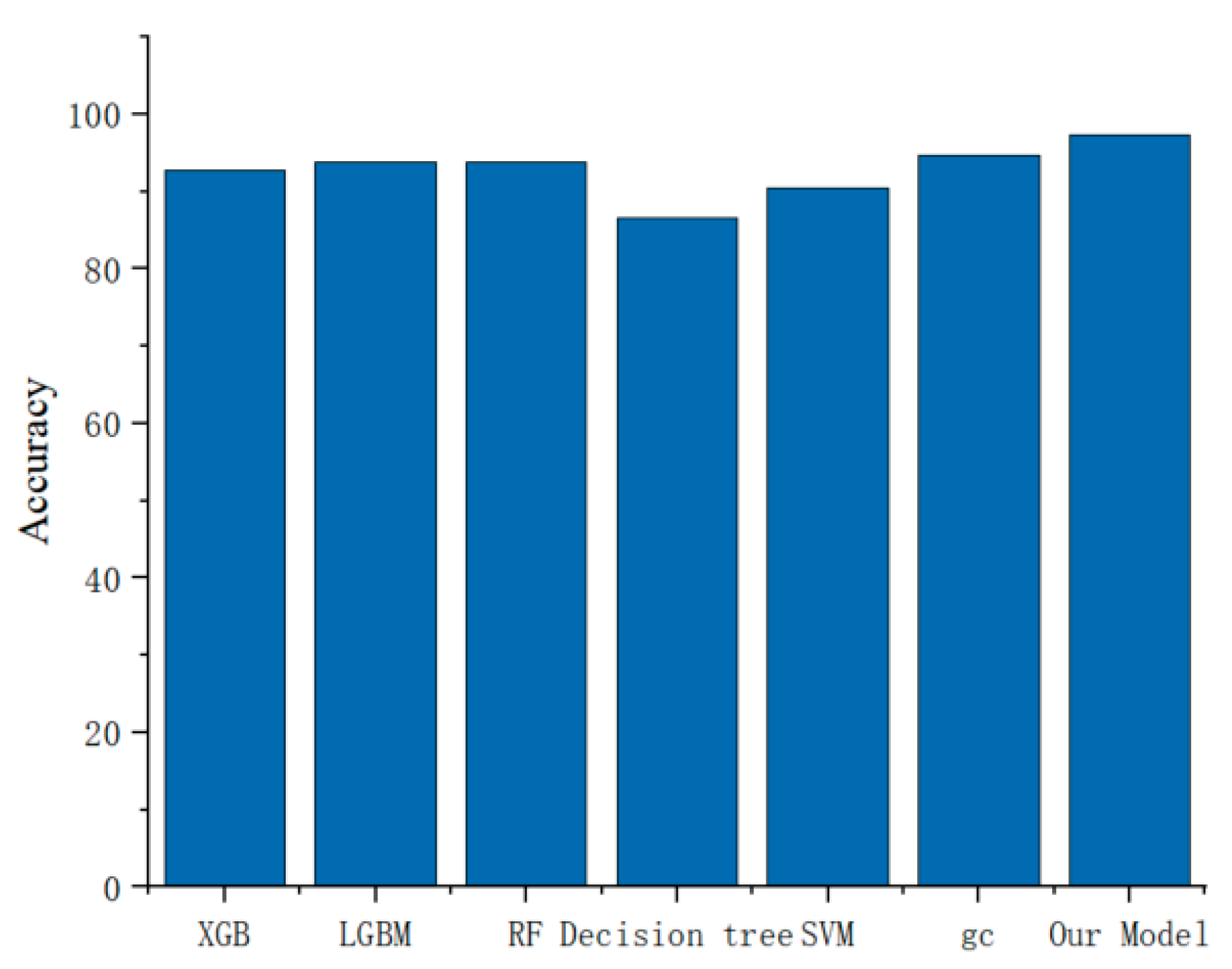
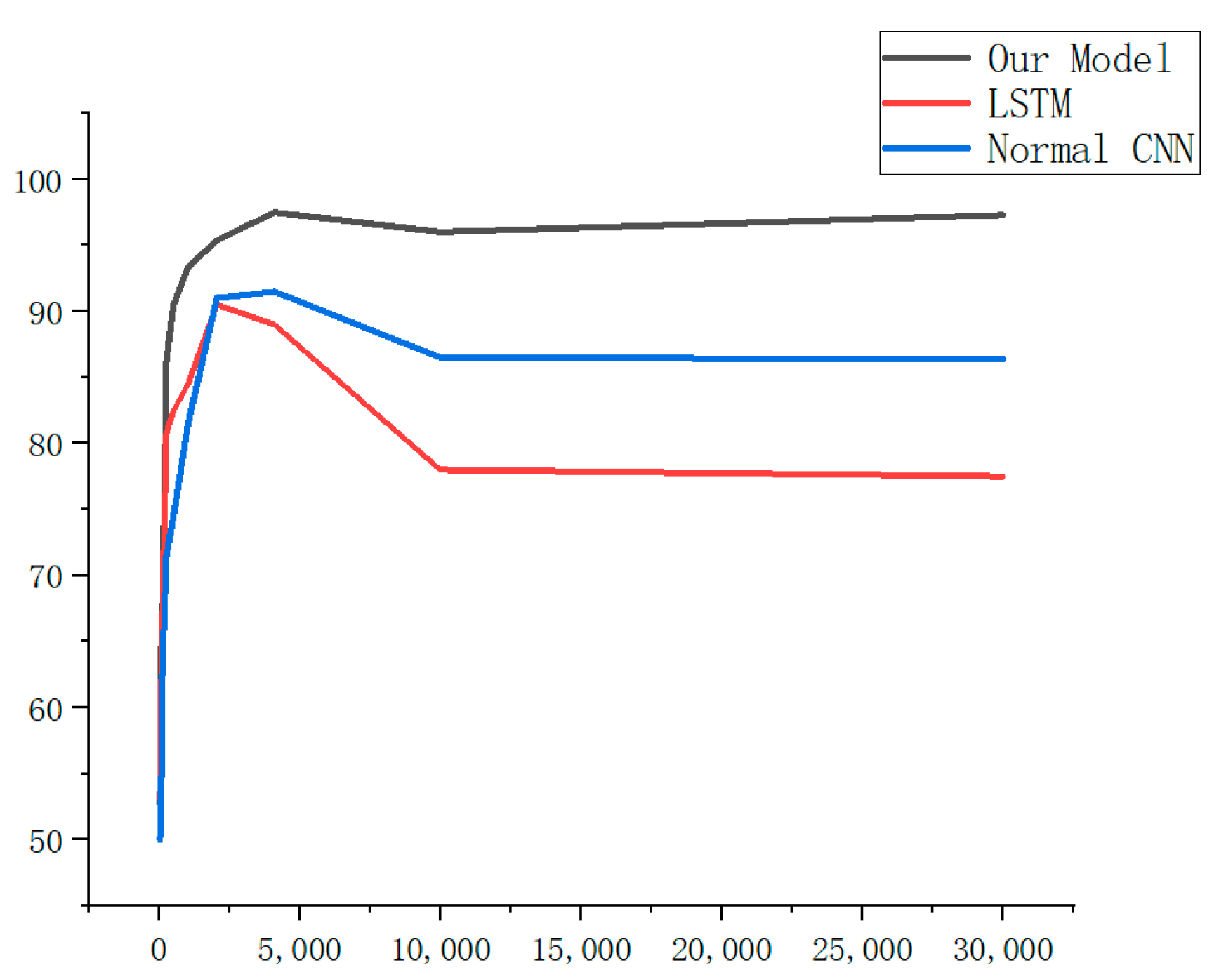
5.6. Comparison of Different Models
5.7. Example of Fileless Malware Detection
6. Summary and Future Prospect
- We create a dataset of in-memory PE files, which includes benign and malicious samples;
- For dynamic files, deep learning can effectively detect memory PE files containing malicious codes;
- The binary data samples can still perform satisfactorily without complicated pre-processing means and can accurately predict the data samples;
- Based on the comparison of the experimental data, the detection effect of the 4096-byte fragment is found to be the best. It is proved that dynamic PE files containing malicious codes can be detected by detecting fragments of the dynamic PE files, thus improving the efficiency of the memory forensics personnel.
Author Contributions
Funding
Data Availability Statement
Conflicts of Interest
References
- Conti, M.; Khandhar, S.; Vinod, P. A few-shot malware classification approach for unknown family recognition using malware feature visualization. Comput. Secur. 2022, 122, 102887. [Google Scholar] [CrossRef]
- Malware Statistics & Trends Report|AV-TEST. AV Test Malware Statistics. Available online: https://www.av-test.org/en/statistics/malware (accessed on 23 December 2022).
- Greenstein, S. The Economics of Information Security and Privacy. J. Econ. Lit. 2014, 52, 1177–1178. [Google Scholar]
- Khalid, O.; Ullah, S.; Ahmad, T.; Saeed, S.; Alabbad, D.A.; Aslam, M.; Buriro, A.; Ahmad, R. An Insight into the Machine-Learning-Based Fileless Malware Detection. Sensors 2023, 23, 612. [Google Scholar] [CrossRef] [PubMed]
- Kara, I. Fileless malware threats: Recent advances, analysis approach through memory forensics and research challenges. Expert Syst. Appl. 2022, 214, 119133. [Google Scholar] [CrossRef]
- Pradip, D.; Pradip, D.; Chakraborty, K. Advances in Number Theory and Applied Analysis; World Scientific: Singapore, 2023. [Google Scholar]
- Franzen, F.; Holl, T.; Andreas, M.; Kirsch, J.; Grossklags, J. Katana: Robust, Automated, Binary-Only Forensic Analysis of Linux Memory Snapshots. In Proceedings of the 25th International Symposium on Research in Attacks, Intrusions and Defenses (RAID 2022), Limassol, Cyprus, 26–28 October 2022; ACM: New York, NY, USA 18p. [Google Scholar] [CrossRef]
- Ligh, M.H.; Case, A.; Levy, J.; Walters, A. The Art of Memory Forensics: Detecting Malware and Threats in Windows, Linux, and Mac memory; John Wiley & Sons: Hoboken, NJ, USA, 2014. [Google Scholar]
- Bozkir, A.S.; Tahillioglu, E.; Aydos, M.; Kara, I. Catch Them Alive: A Malware Detection Approach through Memory Forensics, Manifold Learning and Computer Vision. Comput. Secur. 2021, 103, 061102. [Google Scholar] [CrossRef]
- Majd, A.; Vahidi-Asl, M.; Khalilian, A.; Poorsarvi-Tehrani, P.; Haghighi, H. SLDeep: Statement-level software defect prediction using deep-learning model on static code features. Expert Syst. Appl. 2020, 147, 113156. [Google Scholar] [CrossRef]
- Jiang, F.; Cai, Q.; Lin, J.; Luo, B.; Guan, L.; Ma, Z. TF-BIV: Transparent and Fine-Grained Binary Integrity Verification in the Cloud. In Proceedings of the 35th Annual Computer Security Applications Conference, San Juan, PR, USA, 9–13 December 2019; pp. 57–69. [Google Scholar]
- Zhang, Y.; Liu, Q.Z.; Li, T.; Wu, L.; Shi, C. Research and development of memory forensics. Ruan Jian Xue Bao/J. Softw. 2015, 26, 1151–1172. [Google Scholar]
- Kawakoya, Y.; Shioji, E.; Otsuki, Y.; Iwamura, M.; Miyoshi, J. Stealth Loader: Trace-free Program Loading for Analysis Evasion. J. Inf. Process. 2018, 26, 673–686. [Google Scholar] [CrossRef]
- Uroz, D.; Rodríguez, R.J. On Challenges in Verifying Trusted Executable Files in Memory Forensics. Forensic Sci. Int. Digit. Investig. 2020, 32, 300917. [Google Scholar] [CrossRef]
- Cheng, Y.; Fu, X.; Du, X.; Luo, B.; Guizani, M. A lightweight live memory forensic approach based on hardware virtualization. Inf. Sci. 2017, 379, 23–41. [Google Scholar] [CrossRef]
- Palutke, R.; Block, F.; Reichenberger, P.; Stripeika, D. Hiding process memory via anti-forensic techniques. Forensic Sci. Int. Digit. Investig. 2020, 33, 301012. [Google Scholar] [CrossRef]
- Wang, L. Research on Online Forensics Model and Method Based on Physical Memory Analysis. Ph.D. Thesis, Shandong University, Jinan, China, 2014. [Google Scholar]
- Raff, E.; Barker, J.; Sylvester, J.; Brandon, R.; Catanzaro, B.; Nicholas, C. Malware Detection by Eating a Whole Exe. In Proceedings of the Work-Shops at the Thirty-Second AAAI Conference on Artificial Intelligence, New Orleans, LA, USA, 2–7 February 2018. [Google Scholar]
- Marín, G.; Caasas, P.; Capdehourat, G. Deepmal-deep learning models for malware traffic detection and classification. Data Sci. -Anal. Appl. 2021, 105–112. [Google Scholar]
- Li, H.; Zhan, D.; Liu, T.; Ye, L. Using Deep-Learning-Based Memory Analysis for Malware Detection in Cloud. In Proceedings of the 2019 IEEE 16th International Conference on Mobile Ad Hoc and Sensor Systems Workshops (MASSW), Monterey, CA, USA, 4–7 November 2019; pp. 1–6. [Google Scholar]
- Zhang, Y.; Li, B. Malicious Code Detection Based on Code Semantic Features. IEEE Access 2020, 8, 176728–176737. [Google Scholar] [CrossRef]
- Wadkar, M.; Di Troia, F.; Stamp, M. Detecting malware evolution using support vector machines. Expert Syst. Appl. 2020, 143, 113022. [Google Scholar] [CrossRef]
- Han, W.; Xue, J.; Wang, Y.; Liu, Z.; Kong, Z. MalInsight: A systematic profiling based malware detection framework. J. Netw. Comput. Appl. 2019, 125, 236–250. [Google Scholar] [CrossRef]
- Huang, X.; Ma, L.; Yang, W.; Zhong, Y. A Method for Windows Malware Detection Based on Deep Learning. J. Signal Process. Syst. 2020, 93, 265–273. [Google Scholar] [CrossRef]
- Lu, X.D.; Duan, Z.M.; Qian, Y.K.; Zhou, W. Malicious code classification method based on deep forest. Ruan Jian Xue Bao/J. Softw. 2020, 31, 1454–1464. [Google Scholar]
- Simonyan, K.; Zisserman, A. Very deep convolutional networks for large-scale image recognition. arXiv 2014, arXiv:1409.1556. [Google Scholar]
- Wei, Y.; Chow, K.P.; Yiu, S.M. Insider threat prediction based on unsupervised anomaly detection scheme for proactive forensic investigation. Forensic Sci. Int. Digit. Investig. 2021, 38, 301126. [Google Scholar] [CrossRef]
- Le, H.V.; Ngo, Q.D. V-sandbox for dynamic analysis IoT botnet. IEEE Access 2020, 8, 145768–145786. [Google Scholar] [CrossRef]
- Urooj, U.; Al-Rimy, B.A.S.; Zainal, A.; Ghaleb, F.A.; Rassam, M.A. Ransomware detection using the dynamic analysis and machine learning. Appl. Sci. 2021, 12, 172. [Google Scholar] [CrossRef]
- Shree, R.; Shukla, A.K.; Pandey, R.P.; Shukla, V.; Bajpai, D. Memory forensic: Acquisition and analysis mechanism for operating systems. Mater. Today Proc. 2022, 51, 254–260. [Google Scholar] [CrossRef]
- Jin, X.; Xing, X.; Elahi, H.; Wang, G.; Jiang, H. A Malware Detection Approach using Malware Images and Autoencoders. In Proceedings of the 2020 IEEE 17th International Conference on Mobile Ad Hoc and Sensor Systems (MASS), Virtual, 10–13 December 2020; pp. 1–6. [Google Scholar]
- Singh, J.; Thakur, D.; Gera, T.; Shah, B.; Abuhmed, T.; Ali, F. Classification and analysis of android malware images using feature fusion technique. IEEE Access 2021, 9, 90102–90117. [Google Scholar] [CrossRef]
- Xiao, X.; Zhang, S.; Mercaldo, F.; Hu, G.; Sangaiah, A.K. Android malware detection based on system call sequences and LSTM. Multimed. Tools Appl. 2019, 78, 3979–3999. [Google Scholar] [CrossRef]
- Khalil, F.; Pipa, G. Is deep-learning and natural language processing transcending the financial forecasting? Investigation through lens of news analytic process. Comput. Econ. 2022, 60, 147–171. [Google Scholar] [CrossRef]
- Ren, G.; Yu, K.; Xie, Z.; Liu, L.; Wang, P.; Zhang, W.; Wang, Y.; Wu, X. Differentiation of lumbar disc herniation and lumbar spinal stenosis using natural language processing–based machine learning based on positive symptoms. Neurosurg. Focus 2022, 52, E7. [Google Scholar] [CrossRef] [PubMed]
- Jayasudha, J.; Thilagu, M. A Survey on Sentimental Analysis of Student Reviews Using Natural Language Processing (NLP) and Text Mining. In Proceedings of the Innovations in Intelligent Computing and Communication: First International Conference ICIICC 2022, Bhubaneswar, India, 16–17 December 2022. [Google Scholar]
- Biscione, V.; Bowers, J.S. Convolutional neural networks are not invariant to translation, but they can learn to be. arXiv 2021, arXiv:2110.05861. [Google Scholar]
- Ahmad, I.; Alqarni, M.A.; Almazroi, A.A.; Tariq, A. Experimental Evaluation of Clickbait Detection Using Machine Learning Models. Intell. Autom. Soft Comput. 2020, 26, 1335–1344. [Google Scholar] [CrossRef]


| Fragment Length [Byte] | Convolution Kernel 1 | Max Pool | Convolution Kernel 2 | Convolution Kernel 3 |
|---|---|---|---|---|
| 32 | 5 | 2 | 3 | 2 |
| 64 | 3 | 2 | 4 | 5 |
| 128 | 3 | 2 | 4 | 5 |
| 256 | 3 | 3 | 4 | 5 |
| 512 | 3 | 4 | 4 | 5 |
| 1024 | 3 | 4 | 4 | 5 |
| Fragment Length | Accuracy | Recall | Precision | F-Measure |
|---|---|---|---|---|
| 32 | 52.67 | 11.34 | 83.45 | 20.38 |
| 64 | 63.58 | 39.5 | 78.99 | 52.66 |
| 128 | 68.28 | 66.39 | 69.00 | 67.67 |
| 256 | 86.21 | 84.03 | 87.85 | 86.02 |
| 512 | 90.43 | 84.12 | 96.28 | 89.79 |
| 1024 | 93.34 | 89.91 | 96.83 | 93.24 |
| 2048 | 95.38 | 93.28 | 97.97 | 95.28 |
| 4096 | 97.48 | 96.22 | 98.71 | 97.45 |
| 10,000 | 96.00 | 94.11 | 97.81 | 95.93 |
| 30,000 | 97.27 | 97.90 | 96.68 | 97.29 |
| Fragment Length | Extraction Head | Extraction Tail | Random Extraction |
|---|---|---|---|
| 32 | 52.67 | 51.72 | 63.50 |
| 64 | 63.58 | 59.24 | 67.46 |
| 128 | 68.28 | 59.66 | 69.90 |
| 256 | 86.21 | 60.08 | 70.07 |
| 512 | 90.47 | 65.27 | 70.12 |
| 1024 | 93.34 | 70.37 | 71.79 |
| 2048 | 95.38 | 72.43 | 73.52 |
| 4096 | 97.48 | 73.38 | 74.09 |
| 10,000 | 96.00 | 86.13 | 77.31 |
| 30,000 | 97.27 | 90.97 | 80.04 |
| Fragment Length | Our Model | LSTM | Normal CNN |
|---|---|---|---|
| 32 | 52.67 | 52.99 | 50.00 |
| 64 | 63.58 | 60.49 | 52.36 |
| 128 | 68.28 | 67.99 | 63.46 |
| 256 | 86.21 | 80.75 | 71.45 |
| 512 | 90.47 | 82.47 | 74.50 |
| 1024 | 93.34 | 84.49 | 81.49 |
| 2048 | 95.38 | 90.50 | 90.99 |
| 4096 | 97.48 | 88.99 | 91.49 |
| 10,000 | 96.00 | 77.99 | 86.50 |
| 30,000 | 97.27 | 77.49 | 86.37 |
| Machine Learning Model | Image Width (Pixels) | Accuracy | Recall | Precision | F-Measure |
|---|---|---|---|---|---|
| XGB 1 | 32 | 87.44 | 88.66 | 87.44 | 88.01 |
| LGBM 2 | 32 | 87.44 | 88.72 | 87.44 | 88.03 |
| RF 3 | 32 | 89.82 | 93.34 | 89.82 | 91.50 |
| Decision tree | 32 | 83.85 | 74.01 | 83.85 | 78.42 |
| SVM 4 | 32 | 69.60 | 60.05 | 69.60 | 63.90 |
| DF 5 | 32 | 92.81 | 97.91 | 88.94 | 93.17 |
| XGB | 64 | 87.44 | 88.66 | 87.44 | 88.01 |
| LGBM | 64 | 87.44 | 88.72 | 87.44 | 88.03 |
| RF | 64 | 89.82 | 93.34 | 89.82 | 91.50 |
| Decision tree | 64 | 83.85 | 74.01 | 83.85 | 78.42 |
| SVM | 64 | 69.60 | 60.05 | 69.60 | 63.90 |
| DF | 64 | 92.81 | 97.91 | 88.94 | 93.17 |
| XGB | 128 | 87.44 | 88.66 | 87.44 | 88.01 |
| LGBM | 128 | 87.44 | 88.72 | 87.44 | 88.03 |
| RF | 128 | 89.82 | 93.34 | 89.82 | 91.50 |
| Decision tree | 128 | 83.85 | 74.01 | 83.85 | 78.42 |
| SVM | 128 | 69.60 | 60.05 | 69.60 | 63.90 |
| DF | 128 | 92.81 | 97.91 | 88.94 | 93.17 |
| XGB | 256 | 87.44 | 88.66 | 87.44 | 88.01 |
| LGBM | 256 | 87.44 | 88.72 | 87.44 | 88.03 |
| RF | 256 | 89.82 | 93.34 | 89.82 | 91.50 |
| Decision tree | 256 | 83.85 | 74.01 | 83.85 | 78.42 |
| SVM | 256 | 69.60 | 60.05 | 69.60 | 63.90 |
| DF | 256 | 92.81 | 97.91 | 88.94 | 93.17 |
Disclaimer/Publisher’s Note: The statements, opinions and data contained in all publications are solely those of the individual author(s) and contributor(s) and not of MDPI and/or the editor(s). MDPI and/or the editor(s) disclaim responsibility for any injury to people or property resulting from any ideas, methods, instructions or products referred to in the content. |
© 2023 by the authors. Licensee MDPI, Basel, Switzerland. This article is an open access article distributed under the terms and conditions of the Creative Commons Attribution (CC BY) license (https://creativecommons.org/licenses/by/4.0/).
Share and Cite
Zhang, S.; Hu, C.; Wang, L.; Mihaljevic, M.J.; Xu, S.; Lan, T. A Malware Detection Approach Based on Deep Learning and Memory Forensics. Symmetry 2023, 15, 758. https://doi.org/10.3390/sym15030758
Zhang S, Hu C, Wang L, Mihaljevic MJ, Xu S, Lan T. A Malware Detection Approach Based on Deep Learning and Memory Forensics. Symmetry. 2023; 15(3):758. https://doi.org/10.3390/sym15030758
Chicago/Turabian StyleZhang, Shuhui, Changdong Hu, Lianhai Wang, Miodrag J. Mihaljevic, Shujiang Xu, and Tian Lan. 2023. "A Malware Detection Approach Based on Deep Learning and Memory Forensics" Symmetry 15, no. 3: 758. https://doi.org/10.3390/sym15030758
APA StyleZhang, S., Hu, C., Wang, L., Mihaljevic, M. J., Xu, S., & Lan, T. (2023). A Malware Detection Approach Based on Deep Learning and Memory Forensics. Symmetry, 15(3), 758. https://doi.org/10.3390/sym15030758