A Levenberg-Marquardt Method for Tensor Approximation

Abstract

This paper presents a tensor approximation algorithm, based on the Levenberg–Marquardt method for the nonlinear least square problem, to decompose large-scale tensors into the sum of the products of vector groups of a given scale, or to obtain a low-rank tensor approximation without losing too much accuracy. An Armijo-like rule of inexact line search is also introduced into this algorithm. The result of the tensor decomposition is adjustable, which implies that the decomposition can be specified according to the users’ requirements. The convergence is proved, and numerical experiments show that it has some advantages over the classical Levenberg–Marquardt method. This algorithm is applicable to both symmetric and asymmetric tensors, and it is expected to play a role in the field of large-scale data compression storage and large-scale tensor approximation operations.

1. Introduction

Tensors are widely used in various practical fields, such as video analysis [1,2], text analysis [3], high-level network analysis [4,5,6], data encryption [7,8,9], privacy preserving [10,11,12], and so on. As a form of data storage, tensors usually contain a large amount of data, which sometimes results in great difficulty in solving problems with tensors, for instance, solving tensor equations and so on [13,14,15,16]. Sometimes it will even be impossible to store all entries of a higher-order tensor explicitly. Thus, tensor decomposition and tensor approximation have received more and more attention since the last century, especially with the era of big data coming. Research on tensors has become an attractive topic, and an increasing number of methods [17,18,19,20] for solving tensor decomposition problems have been proposed, such as the widely-used steepest descent method, Newton’s method [21], Gauss–Newton method [22], CANDECOMP/PARAFAC (CP) decomposition [23], Tucker decomposition, Tensor-Train (TT) decomposition, and algebraic method [24,25,26], and so on. We also refer to [27] and the references therein for more related work on low-rank tensor approximation techniques. These methods have rich theoretical achievements and practical applications [28,29,30]. Among them, the CP decomposition is an ideal method in both theory and accuracy aspects, and the specific algorithm is shown in [31]. However, finding the rank of CP decomposition is NP-hard [32], thus there are only several types of tensors that can be decomposed by CP decomposition. Meanwhile, part of them will even increase the data size when the rank is too large. As for TT decomposition [33], this tensor decomposition method is convenient by applying Singular Value Decomposition (SVD), but the accuracy will be greatly degraded.

While the accuracy of tensor decomposition is crucial in practical applications, it is inevitable that errors will occur, as long as it remains within an acceptable range. At the same time, the accuracy of tensor approximation is also important. To reduce the storage and minimize the error, this paper explores a nonlinear least square method for tensor decomposition and low-rank CP tensor approximation, which decomposes or approximates a tensor into/by a sum of rank-one tensors. We first transform the problem into a non-linear least squares problem, so that we can make use of the corresponding theories and techniques of the descent methods. Then, we combine the Levenberg–Marquardt [34,35,36] method with the damped method [37] to obtain a more efficient method for solving this least squares problem. An Armijo-like rule of inexact line search is introduced into this algorithm to ensure the convergence, which makes it different from the Alternating Least Squares (ALS) method. We also optimize the damping parameter to accelerate the convergence rate. It is known that Levenberg–Marquardt method was separately proposed by Kenneth Levenberg [34] and Donald Marquardt [35], and it is an effective method to solve the least squares problems, since it can achieve local quadratic convergence under some certain local error bound assumption. Recently, Levenberg–Marquardt method has been extended to solve tensor-related problems, such as tensor equations, complementarity problems and tensor split feasibility problems [38,39,40,41].

It should be noted that, although the computational efficiency for tensor approximation has been improved by this damped Levenberg–Marquardt method, the iterative process will spend more and more time ineluctably. However, the proposed method still has the following advantages. Firstly, the tensor storage can be significantly reduced since the tensor approximation can be specified according to the users’ requirements. Secondly, the proposed algorithm is universal because the tensor need not satisfy any special properties, and it is applicable to both symmetric and asymmetric tensors. Thirdly, this method is convergent in theory and shows some advantages over the classical Levenberg–Marquardt method in numerical experiments. The primary contribution of this paper is a methodological attempt, and it may play a role in the fields of large-scale data compression storage and large-scale tensor approximation operations, just as other tensor approximation methods.

The rest of this paper is organized as follows. Section 2 introduces the symbols and concepts. Section 3 focuses on the tensor approximation and converts it into a non-linear least squares problems. Then, in order to solve this non-linear least squares problem, an algorithm based on the Levenberg–Marquardt method combined with the damped method, is introduced in Section 3. After that, some numerical experiments are performed to test the feasibility and efficiency of the proposed algorithm in Section 4. Finally, Section 5 concludes the paper.

2. Preliminaries

2.1. Notation

Throughout this paper, vectors are written as italic lowercase letters, such as $x,y,z,\cdots$; the matrices are written as capital letters, such as $A,B,\cdots$; and the tensors are written as $\mathcal{A},\mathcal{B},\cdots$. The symbol $\mathbb{N}$ denotes the set of non-negative integers, the symbol ${\mathbb{N}}_{+}$ denotes the set of positive integers, $\mathbb{R}$ denotes the Euclidean space, and ${\mathbb{R}}^n$ denotes n-dimensional Euclidean space.

Suppose the function $F\left(x\right):{\mathbb{R}}^n⟼\mathbb{R}$ is differentiable and so smooth that the following Taylor expansion is valid:

$$F(x+h)=F\left(x\right)+h^{T}g+\frac{1}{2}{h}^{T}Hh+O\left({\parallel x\parallel }^3\right),$$

(1)

where g in this paper denotes the gradient

$$g\equiv \nabla F\left(x\right)=\left[\begin{array}{c}\frac{\partial F}{\partial x_1}\left(x\right)\\ ⋮\\ \frac{\partial F}{\partial x_n}\left(x\right)\end{array}\right],$$

(2)

and H stands for the Hessian

$$H\equiv {\nabla }^{2}F\left(x\right)=\left[\begin{array}{c}\frac{\partial F^2}{\partial x_i\partial x_j}\left(x\right)\end{array}\right].$$

(3)

Let the function L be defined as follows:

$$F(x+h)\approx L\left(h\right)\equiv F\left(x\right)+h^{T}g+\frac{1}{2}{h}^{T}Hh,$$

(4)

where gain ratio $\varrho$ in the Levenberg–Marquardt method is defined as

$$\varrho =\frac{F\left(x\right)-F(x+h)}{L\left(0\right)-L\left(h\right)}.$$

(5)

For a vector function $f:{\mathbb{R}}^n⟼{\mathbb{R}}^m,m\ge n$, its Taylor expansion is

$$f(x+h)=f\left(x\right)+J\left(x\right)h+O\left({\parallel h\parallel }^2\right),$$

(6)

where $f={(f_1,\cdots ,f_m)}^T$ and $J\in {\mathbb{R}}^{m\times n}$ is the Jacobian, with

$${\left(J\right(x\left)\right)}_{ij}=\frac{\partial f_i}{\partial x_j}\left(x\right).$$

(7)

2.2. Least Squares Problem

A non-linear least squares problem is to find $x^{\ast }$, which is a local minimizer for

$$F\left(x\right)=\frac{1}{2}\sum _{i=1}^m{\left(f_i\left(x\right)\right)}^2,$$

(8)

where $f_i:{\mathbb{R}}^n⟼\mathbb{R},i=1,\cdots ,m,m>n$, are given functions.

2.3. Descending Condition

From a starting point $x_0$, a descent method produces a series of points $x_1,x_2,\cdots$, which (hopefully) converges to $x^{\ast }$, a local minimizer for a given function, and the descending condition is [22]

$$F\left(x_{k+1}\right)<F\left(x_k\right).$$

(9)

2.4. Rank-One Tensors

If an mth-order tensor $\mathcal{A}\in {\mathbb{R}}^{I_1\times I_2\times \cdots \times I_m}$ satisfies

$$\mathcal{A}={\alpha }^{\left(1\right)}\circ {\alpha }^{\left(2\right)}\circ \cdots \circ {\alpha }^{\left(m\right)},$$

(10)

where ${\alpha }^{\left(i\right)}\in {\mathbb{R}}^{I_i},i=1,2,\dots ,m$, and the symbol “∘” means the vector outer product, i.e.,

$${\mathcal{A}}_{i_1{i}_2\cdots i_m}={\alpha }_{i_1}^{\left(1\right)}{\alpha }_{i_2}^{\left(2\right)}\cdots {\alpha }_{i_m}^{\left(m\right)},$$

(11)

then $\mathcal{A}$ is called a rank-one tensor [31].

2.5. Frobenius Norm

For an mth-order tensor $\mathcal{A}\in {\mathbb{R}}^{I_1\times I_2\times \cdots \times I_m}$, the Frobenius norm ${\parallel A\parallel }_F$ is defined as

$${\parallel A\parallel }_F=\sum _{i_1,i_2,\cdots ,i_m}{A}_{i_1{i}_2\cdots i_m}^2.$$

(12)

3. A Damped Levenberg-Marquardt Method for Tensor Approximation

For a given tensor $\mathcal{A}\in {\mathbb{R}}^{I_1\times I_2\times \cdots \times I_m},I_i\in {\mathbb{N}}_{+},i=1,2,\cdots ,m$, the number of the data is denoted as $N_0=I_1\times I_2\times \cdots \times I_m$. Given $R\in \mathbb{R}$, the tensor $\mathcal{A}$ can be approximated by ${\mathcal{A}}^{\ast }$, with

$${\mathcal{A}}^{\ast }={\mathcal{A}}^{\left(1\right)}+{\mathcal{A}}^{\left(2\right)}+\cdots +{\mathcal{A}}^{\left(R\right)},$$

(13)

where ${\mathcal{A}}^{\left(i\right)}\in {\mathbb{R}}^{I_1\times I_2\times \cdots \times I_m},i=1,2,\cdots ,R$, according to (10), are all rank-one tensors as

$${\mathcal{A}}^{\left(i\right)}=u_1^{\left(i\right)}\circ u_2^{\left(i\right)}\circ \cdots \circ u_m^{\left(i\right)}.$$

(14)

Here,

$$u_j^{\left(i\right)}=\left[\begin{array}{c}{u}_{j1}^{\left(i\right)}\\ ⋮\\ u_{j{I}_j}^{\left(i\right)}\end{array}\right],i=1,2,\cdots ,R,j=1,2,\cdots ,m.$$

(15)

Thus, there are $N_d=(I_1+I_2+\cdots +I_m)\times R$ variables in the vectors $u_j^{\left(i\right)},i=1,2,\cdots ,R,j=1,2,\cdots ,m$. In order to approximate $\mathcal{A}$ with ${\mathcal{A}}^{\ast }$, we construct a vector function $f:{\mathbb{R}}^{N_d}⟼{\mathbb{R}}^{N_0}$,

$$f=\left[\begin{array}{c}{f}_{11\cdots 1}\\ f_{21\cdots 1}\\ ⋮\\ f_{I_{1}1\cdots 1}\\ ⋮\\ f_{I_1{I}_2\cdots Im}\end{array}\right],$$

(16)

where

$$f_{i_1{i}_2\cdots i_m}={\mathcal{A}}_{i_1{i}_2\cdots i_m}-\sum _{r=1}^R{u}_{1i_1}^{\left(r\right)}{u}_{2i_2}^{\left(r\right)}\cdots u_{m{i}_m}^{\left(r\right)},i_p=1,2,\cdots ,I_p,p=1,2,\cdots ,m.$$

(17)

Then, we obtain a non-linear least squares problem, which is to find

$$u^{\ast }=argmi{n}_{u}F\left(u\right),$$

(18)

where

$$F\left(u\right)=\frac{1}{2}\sum _{i_1,i_2,\cdots ,i_m}{f_{i_1{i}_2\cdots i_m}}^2=\frac{1}{2}{\parallel f\parallel }^2=\frac{1}{2}{f}^{T}f,$$

(19)

and

$$u={\left[\begin{array}{c}{u}_{11}^1\\ ⋮\\ u_{1I_1}^1\\ u_{11}^2\\ ⋮\\ u_{1I_1}^R\\ u_{21}^1\\ ⋮\\ u_{m{I}_m}^R\end{array}\right]}_{N_d\times 1}.$$

(20)

Concurrently,

$$\frac{\partial F}{\partial u_{qp}^{\left(r\right)}}=\sum _{i=1}^m{f}_{i_1{i}_2\cdots i_m}\frac{\partial f_{i_1{i}_2\cdots i_m}}{\partial u_{qp}^{\left(r\right)}},$$

(21)

combined with (7),

$$J\left(u\right)=\left[\begin{array}{ccc}\frac{\partial f_{11\cdots 1}}{\partial u_{11}^1}& \cdots & \frac{\partial f_{11\cdots 1}}{\partial u_{m{I}_m}^{\left(R\right)}}\\ ⋮& \ddots & ⋮\\ \frac{\partial f_{I_1{I}_2\cdots I_m}}{\partial u_{11}^1}& \cdots & \frac{\partial f_{I_1{I}_2\cdots I_m}}{\partial u_{m{I}_m}^{\left(R\right)}}\end{array}\right],$$

(22)

yields

$$\nabla F\left(u\right)={J\left(u\right)}^{T}f\left(u\right).$$

(23)

Consequently, the number of data decreases from $N_0$ to $N_d$. In other words, when the given number R is small enough so that $N_0>N_d$, then obviously the data size will be reduced.

For obtaining a minimizer of (19), this paper applies the Levenberg–Marquardt method combined with the Damped method, inspired by the high efficiency of the Levenberg–Marquardt method in solving the least squares problem. With the starting point $u_0$, we generate a sequence $\{u_k\}$, which satisfies the descending condition (9). Every step from the current point u consists of: (a) find a descent direction h; (b) find a step size $\alpha >0$ to achieve a proper decrease in the $F-value$; and (c) generate the next point $u_{new}=u+\alpha h$. The iterative direction h (also written as $h\left(u\right)$) is obtained by solving the following equation:

$$(J^{T}J+\mu I)h=-g,$$

(24)

where $J=J\left(u\right)$ in (22), $g=\nabla F\left(u\right)$ in (23), I is the identity matrix, and $\mu$ is the damping parameter.

According to (5), the gain ratio in this damped Levenberg–Marquardt method is

$$\varrho =\frac{F\left(u\right)-F(u+h)}{L\left(0\right)-L\left(h\right)},$$

(25)

for

$$\begin{array}{ccc}L\left(0\right)-L\left(h\right)\hfill & =\hfill & -h^T{J}^{T}f-\frac{1}{2}{h}^T{J}^{T}Jh\hfill \\ \hfill & =\hfill & -\frac{1}{2}{h}^T(2g+(J^{T}J+\mu I-\mu I)h)\hfill \\ \hfill & =\hfill & \frac{1}{2}{h}^T(\mu h-g),\hfill \end{array}$$

(26)

where $h^{T}h$ is positive as long as $h\ne 0$, and we find by (24) that $-h^{T}g=h^T(J^{T}J+\mu I)h>0$. Therefore, whether $\varrho$ is positive or not is determined by $F\left(u\right)-F(u+h)$. Now, the damped Levenberg–Marquardt algorithm is stated as follows (Algorithm 1).

Remark 1.

In this algorithm, we applied the Damped technique, which indicates that when ϱ is small, μ should be increased, and thereby the penalty on large steps will be increased; on the contrary, when ϱ is large, $L\left(h\right)$ is a good approximation to $F(u+h)$ for h, and μ should be decreased. According to [37], the following strategy in general outperforms: if $\varrho >0$, then $\mu :=\mu \times max\{\frac{1}{3},1-{(2\varrho -1)}^3\},\nu :=2$, otherwise $\mu :=\mu \nu ,\nu :=2\nu$. The termination condition is ${\parallel g\parallel }_{\infty }\le {ϵ}_1$. Moreover, steps 9 and 10 show the line search process [41], where $k_{max},\tau ,{ϵ}_1,{ϵ}_2$ are given parameters, and $a_{ii},i=1,2,\cdots ,N_d$ are diagonal elements of matrix $A_{N_d\times N_d}$.

Theorem 1.

If ${\mu }^{\ast }$ is the cluster point of sequence $\{{\mu }_k\}$ generated by Algorithm 1, then $g\left(u^{\ast }\right)=0$.

Proof. 

Suppose the contrary, it holds $g{\left(\mu \right)}^{\ast }\ne 0$. From (24) and ${\mu }^{\ast }$ as the cluster point, we obtain

$${h\left(u^{\ast }\right)}^T{(J\left(u^{\ast }\right)}^{T}J\left(u^{\ast }\right)+\mu I)h\left(u^{\ast }\right)=-{h\left(u^{\ast }\right)}^{T}g\left(u^{\ast }\right)>0,$$

(27)

then ${h\left(u^{\ast }\right)}^{T}g\left(u^{\ast }\right)<0$. According to steps 9 and 10 in Algorithm 1, we have

$$F(u^{\ast }+{\beta }^{m^{\ast }})<F\left(u^{\ast }\right)+\sigma {\beta }^{m^{\ast }}{h\left(u^{\ast }\right)}^{T}g\left(u^{\ast }\right),$$

(28)

for sequence $\{m_i\},\{u_i\}$ generated by steps in Algorithm 1, when $k_i$ is sufficiently large, it holds that

$$F(u_{k_i}+{\beta }^{m^{\ast }})\le F\left(u_{k_i}\right)+\sigma {\beta }^{m^{\ast }}{h\left(u_{k_i}\right)}^{T}g\left(u_{k_i}\right).$$

(29)

By the Armijo criterion, we obtain $m^{\ast }\ge m_{k_i}$, then

$$\begin{array}{ccc}F\left(u_{k_i+1}\right)\hfill & =\hfill & F(u_{k_i}+{\beta }^{m_{k_i}}{h}_{k_i})\hfill \\ \hfill & \le \hfill & F\left(u_{k_i}\right)+\sigma {\beta }^{m_{k_i}}{h\left(u_{k_i}\right)}^{T}g\left(u_{k_i}\right)\hfill \\ \hfill & \le \hfill & F\left(u_{k_i}\right)+\sigma {\beta }^{m^{\ast }}{h\left(u_{k_i}\right)}^{T}g\left(u_{k_i}\right).\hfill \end{array}$$

(30)

It follows that

$$F\left(u_{k_i+1}\right)\le F\left(u_{k_i}\right)+\sigma {\beta }^{m^{\ast }}{h\left(u_{k_i}\right)}^{T}g\left(u_{k_i}\right).$$

(31)

Take the limit, and we have

$$F\left(u^{\ast }\right)\le F\left(u^{\ast }\right)+\sigma {\beta }^{m^{\ast }}{h\left(u^{\ast }\right)}^{T}g\left(u^{\ast }\right),$$

(32)

which implies that ${h\left(u^{\ast }\right)}^{T}g\left(u^{\ast }\right)>0$. This contradicts (27). Therefore, it holds that $g\left(u^{\ast }\right)=0$. □

Algorithm 1 A damped Levenberg–Marquardt method for tensor approximation.

Input: $k:=0;\nu :=2;u:=u_0;\eta =2$            $\sigma :=0.5;\beta :=0.5;m:=0;$            $A:={J\left(u\right)}^{T}J\left(u\right);g:={J\left(u\right)}^{T}f\left(u\right)$            $found:={(\parallel g\parallel }_{\infty }\le {ϵ}_1);\mu :=\tau \times max\{a_{ii}\}$ Output: u 1: while not $found$ and $(k<k_{max})$ do 2:     $k=k+1;$ Solve $(A+\mu I)h=-g$ 3:     if $\parallel h\parallel \le {ϵ}_2(\parallel u\parallel +{ϵ}_2)$ then 4:         $found:=true$ 5:     else 6:         $u_{new}:=u+h$ 7:         $\varrho :=(F\left(u\right)-F\left(x_{new}\right))/(L\left(0\right)-L\left(h\right))$ 8:         if $\varrho >0$ then 9:            while not $F(u+{\beta }^{m}h)<F\left(u\right)+\sigma {\beta }^m{h}^{T}g$ do 10:                $m=m+1$ 11:            $u_{new}:=u+{\beta }^{m}h;m=0$ 12:            $u:=u_{new}$ 13:            $A:={J\left(u\right)}^{T}J\left(u\right);g:={J\left(u\right)}^{T}f\left(u\right)$ 14:            $found:=(\parallel g{\parallel }_{\infty }\le {ϵ}_1)$ 15:            $\mu :=\mu \times max\{\frac{1}{3},1-{(2\varrho -1)}^3\};\nu :=2$ 16:         else 17:            $\mu :=\mu \times \nu ;\nu :=\eta \times \nu$ 18: return result

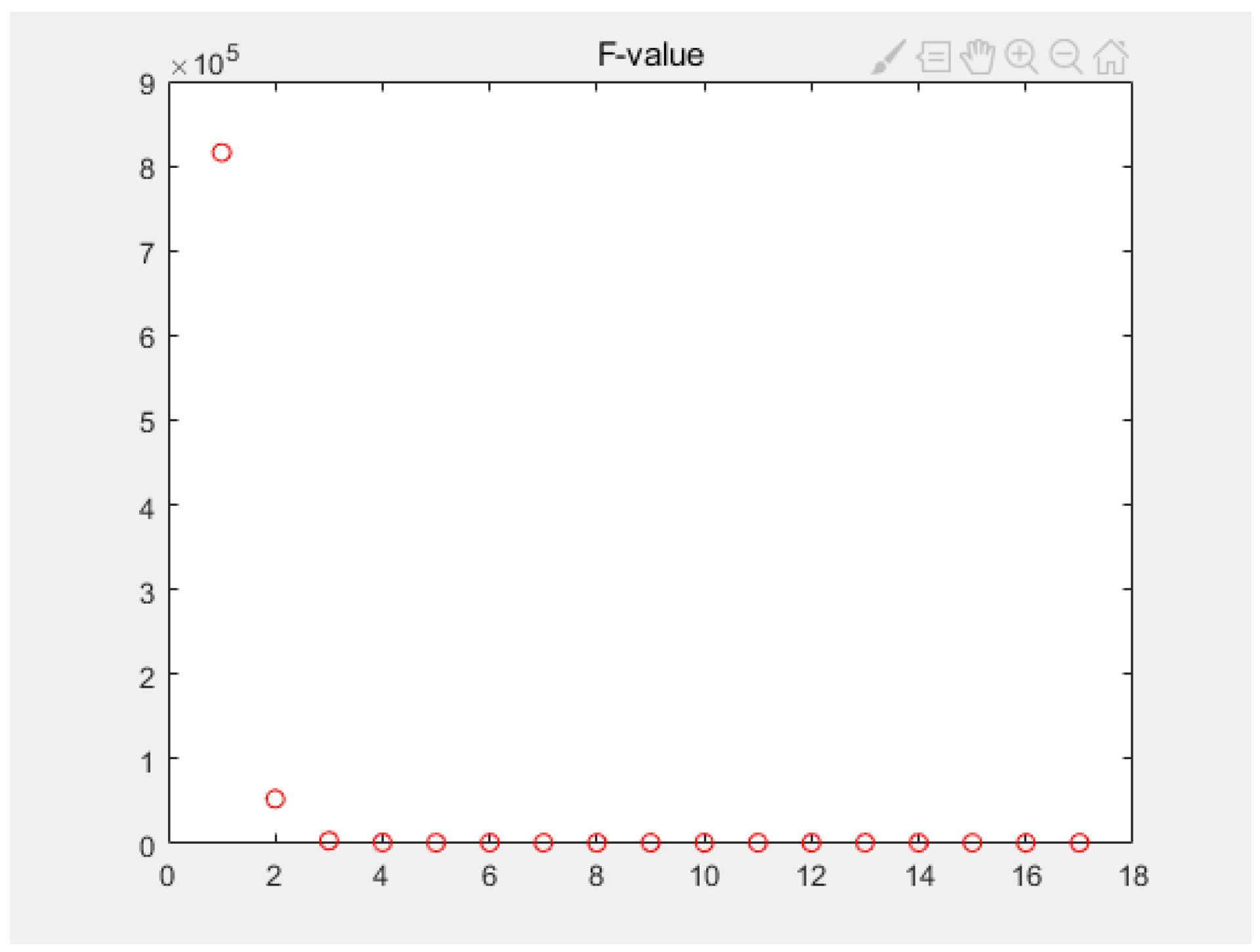
4. Numerical Results

In this section, we perform some numerical experiments to test the proposed method and report the results. We evaluate the error by $\Delta =\parallel \mathcal{A}-{\mathcal{A}}^{\ast }{\parallel }_F$. The computing environment is MATLAB R2018b on a laptop with Intel(R) Core(TM) i7-7700HQ CPU @ 2.80 GHz 2.80 GHz and 16.0 GB RAM.

Example 1.

The tensor $\mathcal{A}\in {\mathbb{R}}^{3\times 3\times 3}$ is generated such that all elements are integers in the range $[1,50]$, with $N_0=27$. Let $R=2$ with $N_d=18$, and parameters are ${ϵ}_1=0.01,{ϵ}_2=0.01,\tau =0.01,$ with $u_0\subset {\mathbb{N}}_{+}\cap [1,10]$, we can obtain the iterative process as follows.

The iterative process for Algorithm 1 for solving this example is reported in

Table 1. Results of Algorithm 1 solving Example 1.

Iteration Steps	Value $\mathit{\mu }$	Value $\parallel \mathit{h}\parallel$	Time Cost (s)	Value $\Delta$
1	$125.67$	$7.715$	$9.5771$	$1.066451\times {10}^3$
2	$41.89$	$5.9723$	$8.9491$	$5.939391\times {10}^2$
3	$13.9633$	$4.4347$	$8.9854$	$3.241196\times {10}^2$
4	$4.6544$	$3.3805$	$8.8872$	$1.750603\times {10}^2$
5	$1.5515$	$3.7187$	$9.2101$	$9.715369\times {10}^1$
⋮	⋮	⋮	⋮	⋮
25	$8.8372\times {10}^{-10}$	$0.2832$	$11.5673$	$3.808415\times {10}^1$
26	$2.9457\times {10}^{-10}$	$0.2559$	$12.3084$	$3.80814\times {10}^1$
27	$9.8191\times {10}^{-11}$	$0.2308$	$11.3772$	$3.807923\times {10}^1$
28	$3.273\times {10}^{-11}$	$0.2079$	$10.5674$	$3.807751\times {10}^1$
29	$3.273\times {10}^{-11}$	$0.1871$	$3.4915$	$3.807751\times {10}^1$

For comparison, the classical Levenberg–Marquardt method with simply $\mu =\parallel F\left(u\right)\parallel$ is also applied to solve this example, and the iterative process is shown in

Table 2. Results of the classical Levenberg–Marquardt method solving Example 1.

Iteration Steps	Value $\mathit{\mu }$	Value $\parallel \mathit{h}\parallel$	Time Cost (s)	Value $\Delta$
1	$1.7023\times {10}^6$	$0.2677$	$8.9846$	$1.845141\times {10}^3$
2	$1.6388\times {10}^6$	$0.2698$	$8.9275$	$1.810389\times {10}^3$
3	$1.5766\times {10}^6$	$0.2718$	$8.9608$	$1.775739\times {10}^3$
4	$1.5159\times {10}^6$	$0.274$	$8.9397$	$1.741189\times {10}^3$
5	$1.4565\times {10}^6$	$0.2762$	$9.2693$	$1.706739\times {10}^3$
⋮	⋮	⋮	⋮	⋮
206	$830.8917$	$0.0517$	$8.9761$	$4.076498\times {10}^1$
207	$829.7662$	$0.0512$	$8.9692$	$4.073736\times {10}^1$
208	$828.6646$	$0.0507$	$9.0058$	$4.071031\times {10}^1$
209	$827.5866$	$0.0502$	$9.0094$	$4.068382\times {10}^1$
210	$826.5316$	$0.0497$	$8.9816$	$4.065788\times {10}^1$

. Obviously, Algorithm 1 has a higher convergence speed than the classical method with simply $\mu =\parallel F\left(u\right)\parallel$. Figure 1 and Figure 2 show the decreasing process of F value when solving this problem by Algorithm 1 and the classical Levenberg–Marquardt method, respectively.

Example 2.

The tensor $\mathcal{A}\in {\mathbb{R}}^{4\times 3\times 4\times 5}$ is generated such that all elements are integers in the range $[1,50]$, with $N_0=240$. Let $R=3$ with $N_d=48$, and parameters are ${ϵ}_1=0.01,{ϵ}_2=0.01,\tau =0.01,$ with $u_0\subset {\mathbb{N}}_{+}\cap [1,10]$. The iterative process is stated in the following

Table 3. Results of Algorithm 1 solving Example 2.

Iteration Steps	Value $\parallel \mathit{h}\parallel$	Total Time Cost (s)	Value $\Delta$
1	$10.4769$	$148.375561$	$1.919757\times {10}^4$
2	$6.9689$	$465.724726$	$5.012392\times {10}^3$
3	$3.9841$	$2570.192530$	$1.086476\times {10}^3$
4	$2.0578$	$5533.349151$	$2.746202\times {10}^2$
5	$1.6461$	$8337.919030$	$2.068849\times {10}^2$
6	$2.0244$	$10861.988487$	$1.861166\times {10}^2$
7	$1.6314$	$42811.813562$	$1.782579\times {10}^2$

. This example shows that Algorithm 1 is also applicable for non-square tensors.

Example 3.

The tensor $\mathcal{A}\in {\mathbb{R}}^{2\times 2\times 2\times 2\times 2}$ is generated such that all elements are integers in the range $[1,50]$, with $N_0=32$. Let $R=2$ with $N_d=20$, and parameters are ${ϵ}_1=0.01,{ϵ}_2=0.01,\tau =0.01,$ with $u_0\subset {\mathbb{N}}_{+}\cap [1,10]$. The costing time for some essential parts in Algorithm 1 is given in

Table 4. Example 3.

Steps	$\parallel \mathit{h}\parallel$	Time for h (s)	Time Cost (s)	Total Time (s)	Value $\Delta$
1	$4.3183$	$1.9449$	$11.9619$	$18.051$	$3.765761\times 4$
2	$3.8025$	$7.9705$	$16.9499$	$35.7049$	$2.210137\times 4$
3	$3.2873$	$46.3806$	$55.1787$	$92.1544$	$1.288507\times 4$
4	$2.7572$	$764.5759$	$773.0252$	$865.2164$	$7.424059\times 3$
5	$2.2295$	$9.7946\times {10}^3$	$9.8077\times {10}^3$	$1.0674\times {10}^4$	$4.207814\times 3$
6	$1.777$	$9.6397\times {10}^3$	$9.6496\times {10}^3$	$2.0325\times {10}^4$	$2.344068\times 3$
7	$1.4312$	$1.1416\times {10}^4$	$1.1426\times {10}^4$	$3.1751\times {10}^4$	$1.279743\times 3$
8	$1.2552$	$9.7942\times {10}^3$	$9.804\times {10}^3$	$4.1556\times {10}^4$	$6.879879\times 2$
9	$1.436$	$1.0784\times {10}^4$	$1.0795\times {10}^4$	$5.2351\times {10}^4$	$3.741665\times 2$

.

Here, the column of “Time for h” states the time for computing h, and that of “Time cost” states the runtime. We see obviously from Table 4 that, solving $\parallel h\parallel$ occupies most of the runtime. Here, a comprehensive algorithm is adopted in this paper by the function “mldivide” in MATLAB R2018b, which includes LU decomposition and so on.

Example 4.

The tensor $\mathcal{A}\in {\mathbb{R}}^{7\times 7\times 3}$ is generated from RGB of some image ($7\times 7$ pixels) shown as follows, with $N_0=147$. Let $R=2$ with $N_d=34$, and parameters are ${ϵ}_1=0.01,{ϵ}_2=0.01,\tau =0.01,$ with $u_0\subset {\mathbb{N}}_{+}\cap [1,10]$. We apply Algorithm 1 to decompose these tensors generated from the images, and obtain their approximating rank-one tensors, then show the corresponding images generated from the approximating tensors (i.e., the restoring images generated from $u^{\ast }$). See Figure 3, Figure 4, Figure 5, Figure 6, Figure 7 and Figure 8. Here, Figure 3, Figure 5, and Figure 7 are the original images, and comparatively, Figure 4, Figure 6 and Figure 8 are the restoring images. The iterative process is stated in

Table 5. Example 4.

Serial Number	Iterative Steps	Time Cost (s)	Value $\Delta$
1	13	$3.8497\times {10}^2$	$1.216391\times {10}^1$
2	8	$2.0676\times {10}^2$	$3.580512\times {10}^2$
3	22	$3.5548\times {10}^3$	$1.216391\times {10}^1$

. The table and Figure 3, Figure 4, Figure 5, Figure 6, Figure 7 and Figure 8 show that Algorithm 1 is applicable for color image tensor decomposition.

From these numerical results, we find that Algorithm 1 can be used in tensor decomposition. Compared with the classical Levenberg–Marquardt method, this damped Levenberg–Marquardt method behaves better in tensor approximation. With the help of the damped technique, the objective function F is descending rapidly. The damped parameter $\mu$ plays an important role in the adjustment of h. By a tensor approximation technique, the data size is obviously decreased; however, the computing speed becomes slower as the size of the tensor increases. The principle reason is that solving the Equation (24) for obtaining h costs the most time.

5. Conclusions

In this paper, we explore a tensor approximation method to reduce the scale of tensor storage, based on nonlinear least squares. It improves the classical Levenberg–Marquardt algorithm by adjusting the damped parameter $\mu$ with the gain ratio $\varrho$, which can speed up the convergence of the algorithm. An Armijo-like line search rule is also introduced into this algorithm to ensure the convergence. Preliminary numerical results show that this tensor decomposition method can help to reduce the data size effectively. Additionally, this method does not require the tensor to satisfy any specific properties, such as supersymmetry [40] and so on. The tensor can be square or non-square, sparse or nonsparse, symmetric or asymmetric. However, the computing time increases rapidly as the size of the tensor increases. By analyzing the results of the numerical experiments, the main reason causing this to happen is that solving the linear equations (step 2 in Algorithm 1) to compute h costs most of the time. How to conquer it still needs further study. Nevertheless, the proposed method still makes some sense in the field of large-scale data compression storage and large-scale tensor approximation operations.

References

1. Li, Q.; Shi, X.; Schonfeld, D. A general framework for robust HOSVD-based indexing and retrieval with high-order tensor data. In Proceedings of the IEEE International Conference on Acoustics, Prague, Czech Republic, 22–27 May 2011. [Google Scholar]
2. Yan, H.Y.; Chen, M.Q.; Hu, L.; Jia, C.F. Secure video retrieval using image query on an untrusted cloud. Appl. Soft Comput. 2020, 97, 106782. [Google Scholar] [CrossRef]
3. Liu, N.; Zhang, B.Y.; Yan, J. Text Representation: From Vector to Tensor. In Proceedings of the IEEE International Conference on Data Mining, Houston, TX, USA, 27–30 November 2005. [Google Scholar]
4. Kolda, T.G.; Bader, B.W.; Kenny, J.P. Higher-Order Web Link Analysis Using Multilinear Algebra. In Proceedings of the 5th IEEE International Conference on Data Mining (ICDM 2005), Houston, TX, USA, 27–30 November 2005. [Google Scholar]
5. Jiang, N.; Jie, W.; Li, J.; Liu, X.M.; Jin, D. GATrust: A Multi-Aspect Graph Attention Network Model for Trust Assessment in OSNs. IEEE Trans. Knowl. Data Eng. 2022. Early Access. [Google Scholar] [CrossRef]
6. Ai, S.; Hong, S.; Zheng, X.Y.; Wang, Y.; Liu, X.Z. CSRT rumor spreading model based on complex network. Int. J. Intell. Syst. 2021, 36, 1903–1913. [Google Scholar] [CrossRef]
7. Liu, Z.L.; Huang, Y.Y.; Song, X.F.; Li, B.; Li, J.; Yuan, Y.L.; Dong, C.Y. Eurus: Towards an Efficient Searchable Symmetric Encryption With Size Pattern Protection. IEEE Trans. Dependable Secur. Comput. 2022, 19, 2023–2037. [Google Scholar] [CrossRef]
8. Gao, C.Z.; Li, J.; Xia, S.B.; Choo, K.K.R.; Lou, W.J.; Dong, C.Y. MAS-Encryption and its Applications in Privacy-Preserving Classifiers. IEEE Trans. Knowl. Data Eng. 2022, 34, 2306–2323. [Google Scholar] [CrossRef]
9. Mo, K.H.; Tang, W.X.; Li, J.; Yuan, X. Attacking Deep Reinforcement Learning with Decoupled Adversarial Policy. IEEE Trans. Dependable Secur. Comput. 2023, 20, 758–768. [Google Scholar] [CrossRef]
10. Zhu, T.Q.; Zhou, W.; Ye, D.Y.; Cheng, Z.S.; Li, J. Resource Allocation in IoT Edge Computing via Concurrent Federated Reinforcement Learning. IEEE Internet Things J. 2022, 9, 1414–1426. [Google Scholar]
11. Liu, Z.L.; Lv, S.Y.; Li, J.; Huang, Y.Y.; Guo, L.; Yuan, Y.L.; Dong, C.Y. EncodeORE: Reducing Leakage and Preserving Practicality in Order-Revealing Encryption. IEEE Trans. Dependable Secur. Comput. 2022, 19, 1579–1591. [Google Scholar] [CrossRef]
12. Zhu, T.Q.; Li, J.; Hu, X.Y.; Xiong, P.; Zhou, W.L. The Dynamic Privacy-Preserving Mechanisms for Online Dynamic Social Networks. IEEE Trans. Knowl. Data Eng. 2022, 34, 2962–2974. [Google Scholar] [CrossRef]
13. Li, X.; Ng, M.K. Solving sparse non-negative tensor equations: Algorithms and applications. Front. Math. China 2015, 10, 649–680. [Google Scholar] [CrossRef]
14. Li, D.H.; Xie, S.; Xu, H.R. Splitting methods for tensor equations. Numer. Linear Algebra Appl. 2017, 24, e2102. [Google Scholar] [CrossRef]
15. Ding, W.Y.; Wei, Y.M. Solving multi-linear systems with M-tensors. J. Sci. Comput. 2016, 68, 689–715. [Google Scholar] [CrossRef]
16. Han, L. A homotopy method for solving multilinear systems with M-tensors. Appl. Math. Lett. 2017, 69, 49–54. [Google Scholar] [CrossRef] [Green Version]
17. Hitchcock, F.L. The expression of a tensor or a polyadic as a sum of products. J. Math. Phys. 1927, 6, 164–189. [Google Scholar] [CrossRef]
18. Hitchcock, F.L. Multiple invariants and generalized rank of a p-way matrix or tensor. J. Math. Phys. 1928, 7, 39–79. [Google Scholar] [CrossRef]
19. Kolda, T.G. Multilinear operators for higher-order decompositions. Sandia Rep. 2006. [Google Scholar] [CrossRef] [Green Version]
20. Sidiropoulos, N.D.; Bro, R. On the uniqueness of multilinear decomposition of N-way arrays. J. Chemom. 2015, 14, 229–239. [Google Scholar] [CrossRef]
21. Goncalves, M.L.N.; Oliveira, F.R. An Inexact Newton-like conditional gradient method for constrained nonlinear systems. Appl. Numer. Math. 2018, 132, 22–34. [Google Scholar] [CrossRef] [Green Version]
22. Madsen, K.; Nielsen, H.B.; Tingleff, O. Methods for Non-Linear Least Squares Problems, 2nd ed.; Technical University of Denmark: Kongens Lyngby, Denmark, 2004; Available online: https://orbit.dtu.dk/en/publications/methods-for-non-linear-least-squares-problems-2nd-ed (accessed on 7 March 2023).
23. Harshman, R.A. Foundations of the PARAFAC procedure: Models and conditions for an “explanatory” multimodal factor analysis. UCLA Work. Pap. Phon. 1970, 16, 1–84. [Google Scholar]
24. Drexler, F. Eine methode zur Berechnung Sämtlicher Lösungen von polynomgleichungssytemen. Numer. Math. 1977, 29, 45–48. [Google Scholar] [CrossRef]
25. Garia, C.; Zangwill, W. Finding all solutions to polynomial systems and other systems of equations. Math. Progam. 1979, 16, 159–176. [Google Scholar] [CrossRef]
26. Li, T. Numerical solution of multivariate polynomial systems by homotopy continuation methods. Acta Numer. 1997, 6, 399–436. [Google Scholar] [CrossRef]
27. Grasedyck, L.; Kressner, D.; Tobler, C. A literature survey of low-rank tensor approximation techniques. Gamm-Mitteilungen 2013, 36, 53–78. [Google Scholar] [CrossRef] [Green Version]
28. Li, J.; Ye, H.; Li, T.; Wang, W.; Lou, W.J.; Hou, Y.; Liu, J.Q.; Lu, R.X. Efficient and Secure Outsourcing of Differentially Private Data Publishing With Multiple Evaluators. IEEE Trans. Dependable Secur. Comput. 2022, 19, 67–76. [Google Scholar] [CrossRef]
29. Yan, H.Y.; Hu, L.; Xiang, X.Y.; Liu, Z.L.; Yuan, X. PPCL: Privacy-preserving collaborative learning for mitigating indirect information leakage. Inf. Sci. 2021, 548, 423–437. [Google Scholar] [CrossRef]
30. Hu, L.; Yan, H.Y.; Li, L.; Pan, Z.J.; Liu, X.Z.; Zhang, Z.L. MHAT: An efficient model-heterogenous aggregation training scheme for federated learning. Inf. Sci. 2021, 560, 493–503. [Google Scholar] [CrossRef]
31. Kolda, T.G.; Bader, B.W. Tensor decompositions and applications. SIAM Rev. 2009, 51, 455–500. [Google Scholar] [CrossRef]
32. Carroll, J.D.; Chang, J.J. Analysis of individual differences in multidimensional scaling via an N-way generalization of “Eckart-Young” decomposition. Psychometrika 1970, 35, 283–319. [Google Scholar] [CrossRef]
33. Oseledets, I.V. Tensor-train decomposition. SIAM J. Sci. Comput. 2011, 33, 2295–2317. [Google Scholar] [CrossRef]
34. Levenberg, K. A method for the solution of certain non-linear problems in least squares. Q. Appl. Math. 1994, 2, 436–438. [Google Scholar] [CrossRef] [Green Version]
35. Marquardt, D. An algorithm for least-squares estimation of nonlinear parameters. SIAM J. Appl. Math. 1963, 11, 431–441. [Google Scholar] [CrossRef]
36. Tichavsky, P.; Phan, H.A.; Cichocki, A. Krylov-Levenberg-Marquardt Algorithm for Structured Tucker Tensor Decompositions. IEEE J. Sel. Top. Signal Process. 2021, 99, 1–10. [Google Scholar] [CrossRef]
37. Nielsen, H.B. Damping Parameter in Marquardt’s Method. IMM. 1999. Available online: https://findit.dtu.dk/en/catalog/537f0cba7401dbcc120040af (accessed on 7 March 2023).
38. Huang, B.H.; Ma, C.F. The modulus-based Levenberg-Marquardt method for solving linear complementarity problem. Numer. Math.Theory Methods Appl. 2018, 12, 154–168. [Google Scholar]
39. Huang, B.H.; Ma, C.F. Accelerated modulus-based matrix splitting iteration method for a class of nonlinear complementarity problems. Comput. Appl. Math. 2018, 37, 3053–3076. [Google Scholar] [CrossRef]
40. Lv, C.Q.; Ma, C.F. A Levenberg-Marquardt method for solving semi-symmetric tensor equations. J. Comput. Appl. Math. 2018, 332, 13–25. [Google Scholar] [CrossRef]
41. Jin, Y.X.; Zhao, J.L. A Levenberg–Marquardt Method for Solving the Tensor Split Feasibility Problem. J. Oper. Res. Soc. China 2021, 9, 797–817. [Google Scholar] [CrossRef]
Figure 1. F-value, μ is generated by Algorithm 1.
Symmetry 15 00694 g001
Figure 2. F-value, μ = F ( u ) by classical L-M method.
Symmetry 15 00694 g002
Figure 3. No.1 yellow and blue color bar original image.
Symmetry 15 00694 g003
Figure 4. No.1 yellow and blue color bar restoring image.
Symmetry 15 00694 g004
Figure 5. No.2 red yellow and blue color bar original image.
Symmetry 15 00694 g005
Figure 6. No.2 red yellow and blue color bar restoring image.
Symmetry 15 00694 g006
Figure 7. No.3 letter E original image.
Symmetry 15 00694 g007
Figure 8. No.3 letter E restoring image.
Symmetry 15 00694 g008