Article

Calculation of Effective Characteristics of a 2D Composite with Rhombic Voids Using an Inhomogeneous Cell Model

1
Chair and Institute of General Mechanics, RWTH Aachen University, Templergraben 64, 52062 Aachen, Germany
2
Department of Information Technology and Information Systems, Dnipro University of Technology, Av. Dmytra Yavornytskoho, 19, 49005 Dnipro, Ukraine
*
Author to whom correspondence should be addressed.
Symmetry 2023, 15(3), 646; https://doi.org/10.3390/sym15030646
Submission received: 7 February 2023 / Revised: 21 February 2023 / Accepted: 1 March 2023 / Published: 4 March 2023
(This article belongs to the Section Engineering and Materials)

Abstract

:
One of the most common approximations in the theory of composite materials is the homogenization theory. The main difficulty in its application lies in solving the cell problem, i.e., the boundary value problem on a periodically repeating element of composite material. For the case of inclusions of large size and with characteristics far superior to those of the matrix, the lubrication approach gives good results. However, the use of such an asymptotic approach is unnatural for the case when the characteristics of the matrix exceed the characteristics of the inclusion. In the presented work, the problem of conductivity for a 2D composite with rhombic voids is considered. The solution of the cell problem is carried out by two methods. First, the lubrication approach is used for this purpose. In addition, a modification of the Schwarz alternating method is proposed. This new approach has been called an “inhomogeneous cell model”. Both methods made it possible to obtain analytical expressions for the effective conductivity. A comparison of the indicated approximate models is carried out, and it is shown that the obtained solutions exactly satisfy Keller’s theorem. The physical foundations of the proposed inhomogeneous cell model are discussed. Its advantage in solving the considered problem is shown.

1. Introduction

The asymptotic homogenization theory [1,2,3], based on the idea of separating rapidly and slowly changing solution components, is currently one of the main methods in the theory of composite materials. The homogenized part of the solution describes the effective characteristics of the composite material. The main problem when using the asymptotic homogenization theory is to solve the cell problem, i.e., boundary value problem for a periodically repeating element of composite media. Usually, various numerical methods are used for this purpose, most often the FEM. Even the term “numerical homogenization” appeared. Analytical solutions are based on the Rayleigh method, the Natanzon–Filshtinsky method, and the method of functional equations [4]. In addition, small parameters are often used, such as the small volume fraction of inclusion or a low-contrast parameter [4,5].
An analytical description of the effective characteristics of the composite is also possible for a high concentration of inclusions. The ratio of the distance between inclusions to the characteristic cell size is then a small parameter. This is the so-called lubrication approach (LA) [6,7,8,9,10,11], which, due to its physical meaning, is applicable to the asymptotic study of the averaged characteristics of composites, with inclusions of large sizes and high conductivity. The essence of LA is to replace the boundary value problem in the original periodically repeated domain of the composite (cell) with a problem in a domain with a simpler geometry. Further, the value of the transformed geometric parameter is considered to be a function of the coordinates, and all the necessary analytical relationships are constructed taking into account this dependence in the original cell of the structure.
The legitimacy and expediency of using LA follows from physical considerations: the heat flux in the region of inclusions (large size and high conductivity) make a contribution to the effective flux much greater than the contribution from the heat flux in the edge zones of the cell—the domain of the matrix, which is much smaller in geometric size and has much smaller conductivity.
The proposal in this paper is that the inhomogeneous cell model (ICM) is destinationed for composites with large inclusions of low conductivity and is, in a sense, an inversion of the LA model. Its physical essence is due to the fact that in composites with low-conductivity inclusions, the intensity of the heat flux will be the highest in the region of the matrix, the conductivity of which significantly exceeds the conductivity of the inclusions.
  • From a physical point of view, the comparison of LA and ICM can be visualized as shown for the cell of the composite in Figure 1a,b.
  • At high conductivity of inclusions, the average conductivity of the composite structure is determined mainly by the conductivity of the region of inclusions. Therefore, the use of LA in this case is justified.
  • If the inclusions are of low conductivity, when finding the averaged parameter of the composite, one cannot then neglect the domain of the matrix, the contribution of which is comparable with the contribution of the inclusions. Therefore, the use of LA is inappropriate here. For this case, we have developed ICM.
Our paper is devoted to the presentation of the essence of the ICM. As an example, we consider a 2D composite with rhombic voids. A comparison of the LA and ICM is carried out and it is shown that the obtained solutions exactly satisfy Keller’s theorem. The physical foundations of the proposed inhomogeneous cell model are discussed. Its advantage in solving the considered problem is shown.
The paper is organized as follows. LA for composites with rhombic inclusions is described in Section 2. Section 3 provides the ICM for 2D composite with rhombic voids. In Section 4, physical interpretation of the ICM is proposed. Finally, Section 5 presents the concluding remarks.

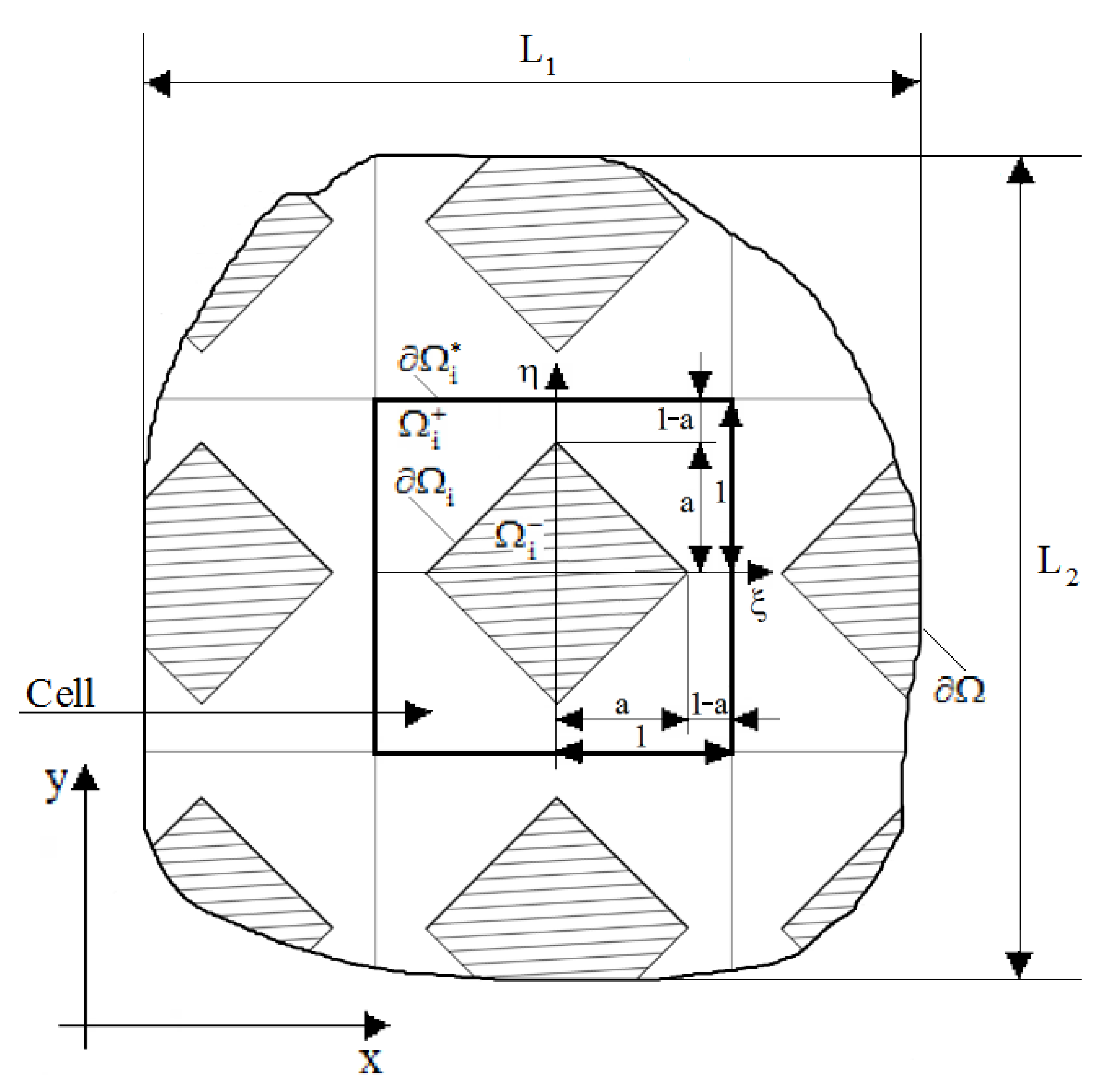
2. LA for Composites with Rhombic Inclusions

The problem of determining the effective thermal conductivity of a two-phase microinhomogeneous material with doubly-periodically arranged large-sized rhombic-section fibers forming a square lattice is under consideration. The cross section of the composite is shown in Figure 2.
The problem of determining the effective thermal conductivity of such a structure is reduced to solving the Poisson equation with conjugation conditions at the phase boundaries and the boundary condition at the outer contour of the composite:
λ + Δ u + = F   in   Ω i + ;   λ Δ u = F ( x , y )   in   Ω i ;
u + = u ,   λ +   u + n = λ   u n   at   Ω i ;
C 1 u + + C 2 u + n = 0   at   Ω ,
where u + , u are the temperature distribution functions in the matrix Ω i + and inclusions Ω i ; λ and λ + are the thermal conductivity of the phases of the composite array; F is the density of heat sources; Ω i , Ω are the contours of the inclusions and the outer contour of the structure, respectively; n is the outer normal to the contour; and C 1   , C 2 are constants.
The function F ( x , y ) changes slowly in the sense that 1 / L i < < 1 . In this case, it is possible to describe the behavior of the composite using the asymptotic homogenization method (AHM) [1,2,3]. A small parameter ε = max     1 / L i < < 1 can be introduced and AHM is applied. In accordance with AHM, based on the multiple scale asymptotic expansions [12], the solution of the problem in the multiply connected domain (1)–(3) is represented as a series in powers of the dimensionless small parameter ε :
u ± = u 0 x ,   y + ε u 1 ± x ,   y ,   ξ ,   η + ε 2 u 2 ± x ,   y ,   ξ ,   η +
where ξ   , η stand for “fast” variables, ξ = x ε , η = y ε .
Thus, the solution is divided into slowly changing and rapidly oscillating parts. Recall that the T-periodic function f ( ε , θ ) is called ε 1 oscillating, if [13] (Appendix 1, pp. 73–74)
0 < C 1 0 T f ε ,   θ 2 d θ C 2 < ,   0 α f ( ε ,   θ ) d θ C ε ,   0 α T ,
where C ,   C 1 ,   C 2 are the positive constants.
The following normalization is used
Ω i + u i + x ,   y ,   ξ ,   η d ξ d η + λ Ω i u i x ,   y ,   ξ ,   η d ξ d η = 0 ,   i = 1 , 2 , 3 ,
Functions u i ± satisfy the periodicity conditions
u i ±   x   , y   , ξ + k   , η + j   = u i ±   x   , y   , ξ   , η ,   i = 1 , 2 , 3 ,
where k , j are integer non-negative numbers.
The cell problem, i.e., the boundary value problem on the minimum periodically repeating element of the composite (Figure 2), takes the form
2 u 1 + ξ 2 + 2 u 1 + η 2 = 0   in   Ω i + ;   2 u 1 ξ 2 + 2 u 1 η 2 = 0   in   Ω i ;
u 1 + = u 1   , u 1 + n ¯ λ   u 1 n ¯ = λ 1   u 0 n   at   Ω i ;
u 1 +     ξ =     1 = u 1 +     ξ = 1 ;   u 1 + ξ     ξ =     1 = u 1 + ξ     ξ = 1 ;
u 1 +     η =     1 = u 1 +     η = 1 ;   u 1 + η     η =     1 = u 1 + η     η = 1 ,
where λ = λ λ + .
First of all, the solution of the problem on the cell (8)–(11) for a composite with inclusions of large sizes a > > 0 of high conductivity λ > > 1 using the LA model is obtained.
Let us separate the heat fluxes in the direction of the coordinate axes ξ   , η and consider one of them in the direction of the axis O η (due to the symmetry of the problem, this is not important). The functions of temperature distribution in the matrix Ω i + and the inclusion Ω i are denoted u 1 η + and u 1 η . With inclusion sizes close to the maximum, a = 1 rhombic inclusions almost touch each other, i.e., 1 a 0 . Consequently, it is within this domain, near almost touching inclusions of high conductivity, that the maximum heat fluxes will be in the composite.
These physical considerations determine the legitimacy and expediency of using LA, which allows us to consider a geometrically simpler problem, namely: to replace the rhombic contour of the inclusion with a square one with side a .
Due to the symmetry of the structure and boundary conditions, we consider the ½ of transformed cell (at η 0 ), denoting, respectively, the domains of the matrix and inclusions Ω i 1 + and Ω i 1 . In accordance with the general idea of the LA method, we take its transformed domain as the calculation model of a cell, with the exception of the edge zones (Figure 3).
Within the framework of the LA, the local problems (8)–(11) can be transformed taking into account the following considerations:
(1) In the domain of the matrix Ω i 1 + of the transformed cell Ω i 1 = Ω i 1 + Ω i , the variables ξ   , η have a different scale of change:
a η 1 ; a ξ a ,
i.e.,
η < < ξ   at   a 1
This means that ξ and η can be treated as “slow” and “fast” variables, respectively.
Then, as follows from [14], for the temperature distribution function in the matrix u 1 η + , one obtains:
2 u 1 η + ξ 2 < < 2 u 1 η + η 2   in   Ω i 1 +
(2) Due to the symmetry of the cell with respect to the axis O ξ , the temperature distribution function in the inclusions u 1 η satisfies the condition:
u 1 η = 0   at   η = 0
(3) As shown in [1], the periodicity conditions (11) for the function u 1 η + can be represented as follows:
u 1 η + = 0   at   η = 1 .
Thus, the local problems (8)–(11) takes the form:
2 u 1 η + η 2 = 0   in   Ω i 1 + ;
2 u 1 η ξ 2 + 2 u 1 η η 2 = 0   in   Ω i ;
u 1 η + = u 1 η   , u 1 η + η λ u 1 η η = λ 1 u 0 η   at   η = a ;
u 1 η + = 0   at   η = 1
u 1   η = 0   at   η = 0 .
Then the solution of the original problem is divided into two stages.
(1) At the first stage, the solution of the local problems (17)–(21) is determined in the transformed domain of the cell.
The general solutions of Equations (17) and (18) have the form, respectively:
u 1 η + = A 0 + B 0 η ;
u 1 η = C 0 + D 0 η + n = 1   C n cosh   π n η + D n sinh   π n η cos   π n ξ + C ¯ n cosh   π n η + D ¯ n sinh   π n η sin   π n ξ ,
where A 0 ,   B 0 ,   C 0 ,   D 0 ,   C n ,   D n ,   C ¯ n ,   D ¯ n   n = 1   ,   2   ,   are the constants, determined from conjugation conditions (19) and boundary conditions (20) and (21).
From the conjugation conditions (19), it follows: C n = D n = C ¯ n = D ¯ n = 0 ,   n = 1 ,   2 ,     , since expression (22) contains only zero terms in the expansion of the function u 1   η + into a Fourier series in the variable ξ .
Using the symmetry condition (21), one obtains C 0 = 0 .
The constants A 0   , B 0   , D 0 are determined from conditions (19) and (20):
A 0 = 1 λ Δ u 0 y ,   B 0 = 1 λ Δ u 0 y ,   D 0 = 1 Δ u 0 y ,
where
Δ = λ λ 1   a 1 .
The final solution to the boundary value problems (17)–(21) is written as follows:
u 1 η + = λ 1 η 1 a λ λ 1 a u 0 y ;   u 1 η = λ 1 1 a η λ λ 1 a u 0 y .
The expressions of the functions u 1   ξ +   , u 1   ξ that determine the heat flux in the direction of the axis O ξ are obtained by changing the variables:
u 1 ξ + = u 1 η + ,   u 1 ξ = u 1 η   u 0 y u 0 x ,   η ξ .
(2) At the second stage of the solution, we consider the inclusion size a as a function of the coordinate ξ (Figure 3)
a ξ = a ξ
The averaging operator is
m   Φ ± x ,   y = 1 Ω i *   [ Ω i + Φ + x ,   y ,   ξ ,   η d ξ d η + λ Ω i Φ x ,   y ,   ξ ,   η d ξ d η ] ,
where Ω i * = Ω i + Ω i .
Apply operator m [ ] to the equation
2 u 0 x 2 + 2 u 0 y 2 + 2 2 u 1 + x ξ + 2 2 u 1 + y η + 2 u 2 + ξ 2 + 2 u 2 + η 2 + λ   2 u 0 x 2 + 2 u 0 y 2 + 2 2 u 1 x ξ + 2 2 u 1 y η + 2 u 2 ξ 2 + 2 u 2 η 2 = F ,
where
u 1 + = u 1 ξ + + u 1 η + ,   u 1 = u 1 ξ + u 1 η ,
and one obtains this.
As a result, one obtains the following homogenized equation:
q = 1 Ω i * [ Ω i + 2 u 0 x 2 + 2 u 0 y 2 + 2 u 1 + x ξ + 2 u 1 + y η d ξ d η + λ Ω i 2 u 0 x 2 + 2 u 0 y 2 + 2 u 1 x ξ + 2 u 1 y η d ξ d η ] = F ,
where integration is performed over the area of the cell with a rhombic inclusion, taking relation (28) into account, i.e., assuming the size of the inclusion a to be a variable function of the coordinate ξ .
After performing the necessary transformations, the homogenized coefficient is obtained from the relation
q = 1 Ω i * [ Ω i + + λ Ω i + λ 1 Ω   i + a ξ λ λ 1   a ξ d ξ d η + λ λ 1 Ω i a ξ 1 λ λ 1 a ξ d ξ d η ] = F
as follows:
q = 1 a + λ λ 1   ln λ λ λ 1 a

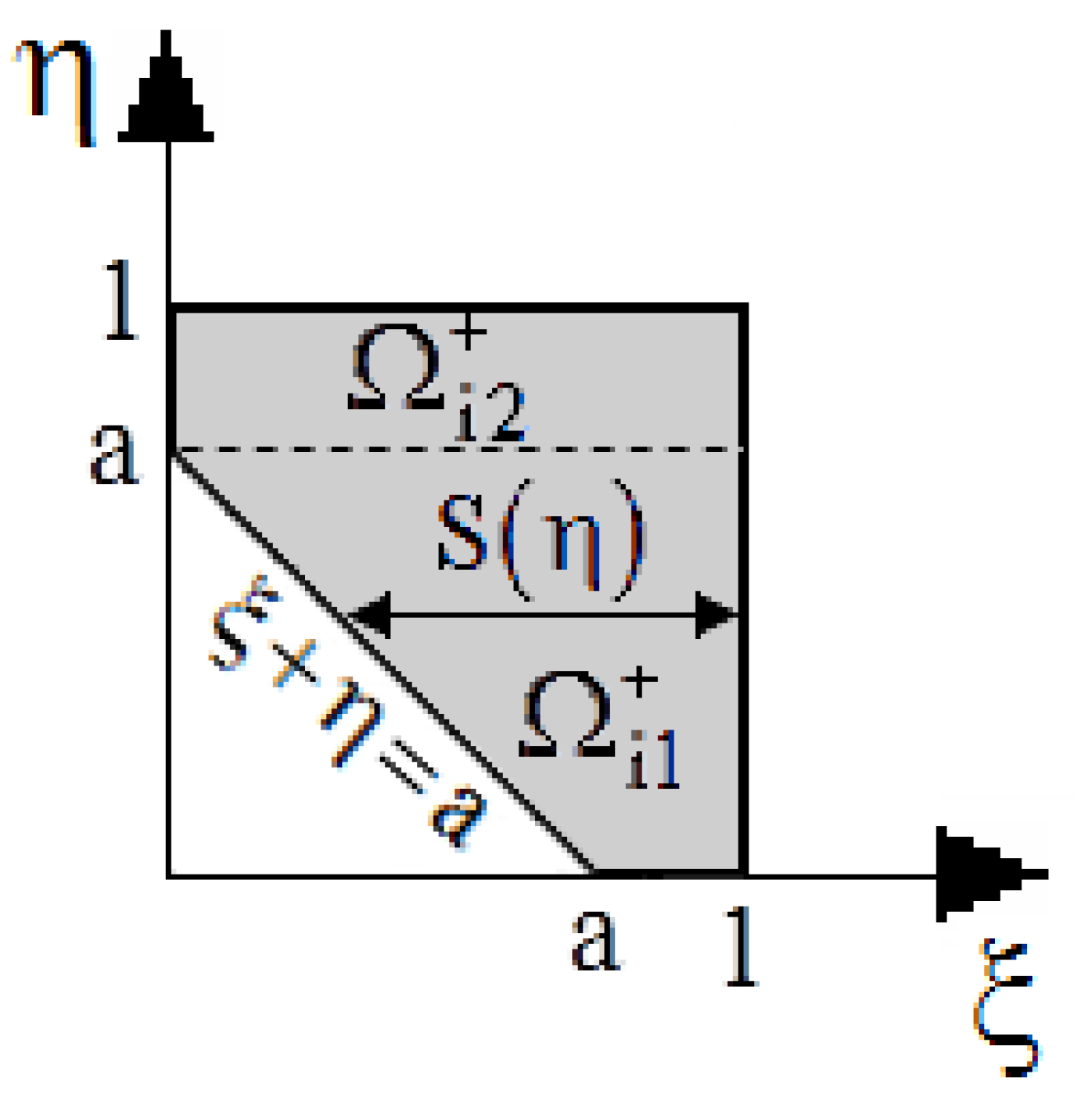
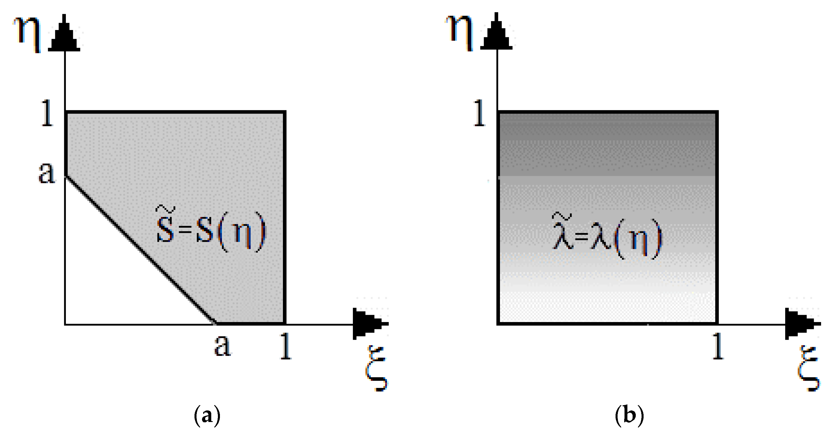
3. ICM for 2D Composite with Rhombic Voids

Consider now a composite array with large rhombic cavities, a > > 0 . Due to symmetry, one can restrict ourselves to the ¼ part of the cell for which ξ 0   , η 0 (Figure 4).
Consider the heat flux in the direction of the axis O η for the case under consideration λ = 0   , and the problem on the cell (8)–(11) for the function u 1 η + takes the form:
2 u 1 η + ξ 2 + 2 u 1 η + η 2 = 0   in   Ω i + ;
u 1 η + n ¯ + u 0 n = 0   at   ξ + η = a ;
u 1 η + = 0   at   η = 0 ;
u 1 η + = 0   at   η = 1 .
The mathematical apparatus used below can be interpreted as the Schwarz alternating method [15], the essence of which is to alternatively satisfy the boundary conditions on cell contours.
To solve problems (35)–(38), successive approximations are used.
The first approach: the solution of the boundary value problems (35)–(38) is obtained from relation (26) at λ = 0 :
u 1 η + 1 = 1 η u 0 y .
This solution:
  • Satisfies the periodicity condition (38).
  • Does not satisfy the symmetry condition (37).
  • Exactly satisfies the condition (36).
Regarding the second approximation, consider the domain of the cell shown in Figure 5.
One can represent the solution of the second approximation u 1 η + 2 in the form:
u 1 η + 2 = u 11 η + 2 + u 12 η + 2 ,
where:
  • the function u 11 η + 2 is defined as the conductivity of a rod of variable cross section S η (domain Ω i 1 + ) from the equation:
    d d η S η d u 11 η + 2 d η = 0 ,
    where
    S η = η + 1 a ,   0 η a ,
    1 a S η = 1 :   S η = 1 a ; η = 0 S η = 1 ; η = a ;
  • The function u 12   η +   2 is defined as the conductivity of a rod of constant cross section (domain Ω i 2 + ) from the equation:
    d 2 u 12 η + 2 d η 2 = 0 .
The u 11 η + 2 and u 12 η + 2 functions must satisfy the conjugation conditions at η = a :
u 11 η + 2 = u 12 η + 2 ,   d u 11 η + 2 d η = d u 12 η + 2 d η   at   η = a .
The solution of the second approximation (40):
  • Must remove residuals, which are given by the solution of the first approximation u 1 η + 1 (39) on the contour η = 0 :
    u 1 η + 1 + u 11 η + 2 = 0   at   η = 0 ,
    or
    u 11 η + 2 = u 1 η + 1   at   η = 0 ;
  • The periodicity condition on the contour η = 1 must be satisfied:
    u 1 η + 1 + u 12 η + 2 = 0   at   η = 1 .
Since u 1 η + 1 = 0 at η = 1 , then:
u 12 η + 2 = 0   at   η = 1 ;
  • On the boundary ξ + η = a , the relation u 1 η + = u 1 η + 1 + u 1 η + 2 does not satisfy condition (36), because u 1 η + 2 n ¯ 0 at ξ + η = a .
The corresponding residuals are removed by solving the next approximation.
The general solution of Equation (44) has the form:
u 12 η + 2 = C 1 + C 2 η .
Next, the general solution of Equation (41) can be written as follows:
d d η η + 1 a   d u 11 η + 2 d η = 0 η + 1 a   d u 11 η + 2 d η = C 3 d u 11 η + 2 d η = C 3 η + 1 a ,
i.e.,
u 11 η + 2 = C 3   d η η + 1 a = C 3   ln η + 1 a + C 4 .
We find the integration constants C 1 C 4 in expressions (50) and (52) from conditions (45), (47), and (49):
C 1 + C 2 a = C 4 C 2 = C 3 C 3   ln 1 a + C 4 = 1 C 1 + C 2 = 0 .
The solution of the system of Equation (53) has the form:
C 1 + C 2 a = C 4 C 2 = C 3 C 3   ln 1 a + C 4 = 1 C 1 + C 2 = 0 ,
where
Δ = 1 a + ln 1 a 1 .
Using the averaging operator m [ ] at λ = 0 , one can integrate each of the functions in its domain of definition:
Ω i 2 u 0 y 2 d ξ d η + Ω i 2 u 1 η + 1 y η d ξ d η + Ω i 1 2 u 11 η + 2 y η d ξ d η + Ω i 2 2 u 12 η + 2 y η d ξ d η = 0 a d η a η 1 2 u 0 y 2 + 2 u 1 η + 1 y η + 2 u 11 η + 2 y η d ξ + a 1 d η 0 1 2 u 0 y 2 + 2 u 1 η + 1 y η + 2 u 12 η + 2 y η d ξ = C 3 a + C 2 1 a 2 u 0 y 2 ,
From this equation, one obtains the effective coefficient q in the form:
q = 1 1 a + ln 1 a 1 .
Based on LA for a composite with large rhombic inclusions a 1 and high conductivity λ > > 1 for the effective thermal conductivity parameter expression (34) was obtained, from which, in the limiting case λ , it follows:
q = 1 a + ln 1 a 1 .
Comparing relations (57) and (58) found, respectively, by the LA and by the ICM, one obtains:
q λ = 1 q λ = 0 .
Thus, Keller’s theorem [16] holds exactly.

4. ICM: Physical Interpretation

Above, a homogeneous rod of conductivity λ + with a variable cross section S ˜ is considered, when
λ + = c o n s t ;
S ˜ = S η = η + 1 a .
The following model will be the equivalent to it: a rod of constant cross section S + with reduced (averaged over the section) conductivity λ ˜ (Figure 6):
S = 1 ;
λ ˜ = λ η = λ + η + 1 a + λ a η 1 = λ + η + 1 a .
Indeed, for each of these models (60)–(63)
λ S = λ + η + 1 a ,
and the general equation of thermal conductivity of the rod for the stationary case
d d η λ S d u d η = 0
reduces to the above equation:
d d η λ + η + 1 a d u d η = 0 ,
or
d d η η + 1 a d u d η = 0 .

5. Conclusions

In this paper, the conductivity problem for 2D composite with rhombic voids is under consideration. The asymptotic homogenization method is used. The main goal is to solve the cell problem analytically and obtain simple expressions for the effective conductivity.
The solution of the cell problem is carried out by two methods. First, the lubrication approach is used for this purpose. In addition, a modification of the Schwarz alternating method is proposed. This new approach has been called an “inhomogeneous cell model”. Both methods made it possible to obtain analytical expressions for the effective conductivity.
A comparison of the indicated approximate models is carried out, and it is shown that the obtained solutions exactly satisfy Keller’s theorem. The physical foundations of the proposed inhomogeneous cell model are discussed. Its advantage in solving the considered problem is shown.
In the future, it is of interest to generalize the above approach to the case of a composite with inclusions of low but not zero conductivity ( 0 < λ < < 1 ).

Author Contributions

Conceptualization, I.A.; methodology, I.A., G.S. and S.K.; investigation, I.A., S.K. and G.S.; writing and original draft preparation, I.A. and S.K.; software, G.S.; writing, review, and editing, I.A. and S.K.; formal analysis, G.S. and S.K. All authors have read and agreed to the published version of the manuscript.

Funding

This research received no external funding.

Institutional Review Board Statement

Not applicable.

Informed Consent Statement

Not applicable.

Data Availability Statement

Data are contained within the article.

Conflicts of Interest

The authors declare no conflict of interest.

References

  1. Panasenko, G. Multi-Scale Modelling for Structures and Composites; Springer: Berlin/Heidelberg, Germany, 2005. [Google Scholar]
  2. Marchenko, V.A.; Khruslov, E.Y. Homogenization of Partial Differential Equations; Birkhäuser: Boston, MA, USA, 2005. [Google Scholar]
  3. Kolpakov, A.A.; Kolpakov, A.G. Capacity and Transport in Contrast Composite Structures: Asymptotic Analysis and Applications; CRC Press: Boca Raton, FL, USA, 2009. [Google Scholar]
  4. Mityushev, V.; Andrianov, I.; Gluzman, S.L.A. Filshtinsky’s contribution to Applied Mathematics and Mechanics of Solids. In Mechanics and Physics of Structured Media. Asymptotic and Integral Equations Methods of Leonid Filshtinsky; Andrianov, I., Gluzman, S., Mityushev, V., Eds.; Academic Press: New York, NY, USA, 2022; pp. 1–40. [Google Scholar]
  5. Movchan, A.B.; Movchan, N.V.; Poulton, C.G. Asymptotic Models of Fields in Dilute and Densely Packed Composites; Imperial College Press: London, UK, 2002. [Google Scholar]
  6. Milton, G. The Theory of Composites; Cambridge University Press: Cambridge, UK, 2009. [Google Scholar]
  7. Christensen, R.M. Mechanics of Composite Materials; Dover Publications: Mineola, NY, USA, 2005. [Google Scholar]
  8. Andrianov, I.V.; Awrejcewicz, J.; Danishevskyy, V.V. Asymptotical Mechanics of Composites. Modelling Composites without FEM.; Springer Nature: Cham, Switzerland, 2018. [Google Scholar]
  9. Panton, R.L. Incompressible Flow, 3rd ed.; Wiley: New York, NY, USA, 2005. [Google Scholar]
  10. Andrianov, I.V.; Awrejcewicz, J.; Starushenko, G.A. Asymptotic models and transport properties of densely packed, high-contrast fibre composites. Part I: Square lattice of circular inclusions. Compos. Struct. 2017, 179, 617–627. [Google Scholar] [CrossRef]
  11. Andrianov, I.V.; Awrejcewicz, J.; Starushenko, G.A. Asymptotic models for transport properties of densely packed, high-contrast fibre composites. Part II: Square lattices of rhombic inclusions and hexagonal lattices of circular inclusions. Compos. Struct. 2017, 180, 351–359. [Google Scholar] [CrossRef]
  12. Awrejcewicz, J.; Starosta, R.; Sypniewska-Kamińska, G. Asymptotic Multiple Scale Method in Time Domain Multi-Degree-of-Freedom Stationary and Nonstationary Dynamics; CRC Press: Boca Raton, FL, USA, 2022. [Google Scholar]
  13. Vishik, M.I.; Lyusternik, L.A. The asymptotic behaviour of solutions of linear differential equations with large or quickly changing coefficients and boundary conditions. Russ. Math. Surv. 1960, 15, 23–91. [Google Scholar] [CrossRef]
  14. Batchelor, G.K.; O’Brien, R.W. Thermal or electrical conduction through a granular material. Proc. R. Soc. Lond. A Math. Phys. Sci. 1977, 355, 313–333. [Google Scholar]
  15. Drygaś, P.; Gluzman, S.; Mityushev, V.; Nawalaniec, W. Applied Analysis of Composite Media: Analytical and Computational Results for Materials Scientists and Engineers; Woodhead Publishing: Cambridge, UK, 2020. [Google Scholar]
  16. Keller, J.B. A theorem on the conductivity of a composite medium. J. Math. Physics 1964, 5, 548–549. [Google Scholar] [CrossRef]
Figure 1. The distribution of heat fluxes in the cell of the composite in the case of inclusions: (a) high conductivity; (b) low conductivity.
Symmetry 15 00646 g001
Figure 2. Cross section of a composite with rhombic fibers.
Symmetry 15 00646 g002
Figure 3. LA model for rhombic inclusions.
Symmetry 15 00646 g003
Figure 4. Quarter-cell of composite with rhombic voids.
Symmetry 15 00646 g004
Figure 5. Cell domain representation in ICM.
Symmetry 15 00646 g005
Figure 6. Equivalent inhomogeneous models. (a) Geometrically inhomogeneous model. (b) Physically inhomogeneous model.
Symmetry 15 00646 g006
Disclaimer/Publisher’s Note: The statements, opinions and data contained in all publications are solely those of the individual author(s) and contributor(s) and not of MDPI and/or the editor(s). MDPI and/or the editor(s) disclaim responsibility for any injury to people or property resulting from any ideas, methods, instructions or products referred to in the content.

