The Metastable State and the Finite-Size Effect of the First-Order Phase Transition

Abstract

In the QCD, a transition restoring the chiral symmetry occurs at a high temperature and density. Searching for the signals of the QCD phase transition is one of the goals of the current relativistic heavy-ion physics programs. The metastable state is a unique feature of the first-order phase transition. Using the van der Waals equation of state, the role of the metastable state in finite-size effects is analyzed. It is found that the finite-size effects of the first-order phase transition are closely related to the metastable state. Metastability can be observed in the distribution of the order parameters and the probability of its occurrence depends on the system scale. A sizable probability of the metastability requires a small enough system size. The possibility of observing the metastability in the RHIC/BES is discussed.

1. Introduction

In the 1970s, T.D. Lee et al. [1,2] predicted that through high-energy heavy-ion collisions, it was possible to form a high-temperature and/or high-density environment so that a new state of matter—quark gluon plasma (QGP) [3,4]—would be produced. Since then, great theoretical and experimental progress has been made in the field. In the 2000s, the relativistic heavy-ion experiments, in particular the Relativistic Heavy-Ion Collider (RHIC) in the Brookheaven National Laboratory with a collision energy of several hundred GeV, had observed the parton (quark and gluon) degrees of freedom [5,6,7,8]. It is widely believed that a strongly coupled QGP has been formed. The discovery of the QGP phase is a milestone in heavy-ion physics. However, the phase boundary between the hadron phase and the QGP phase has not been conclusively mapped yet, challenging the theory and experiment.

Consider $N_f$ flavors of massless quarks which couple in the fundamental representation of a $SU(N_c$) color gauge group. The flavor symmetry of the quantum theory is $G_f=Z_A\left(N_f\right)\times SU\left(N_f\right)\times SU\left(N_f\right)$. At zero temperature, the chromodynamic vacuum spontaneously breaks $G_f$ to $SU\left(N_f\right)$, while at a high temperature, the full chiral symmetry is restored to the vacuum [9]. Lattice QCD calculations at a high temperature indicate that the restoration of the spontaneously broken chiral symmetry with a physical quark mass is a smooth crossover at zero baryon chemical potential [10], while several QCD-based models predict a first-order phase transition at a high baryon chemical potential [11,12,13,14,15]. The existence of the critical point, which terminates the first-order phase transition line in the QCD phase diagram, is expected and being searched for in the ongoing heavy-ion experiments.

High cumulants of conserved charges are sensitive observables to the critical point [16,17,18]. Their sign or the change in the sign can signal the critical point. Especially, the fourth-order cumulant (kurtosis) should show a non-monotonic energy dependence when the chemical freeze-out line gets close to the critical point [19]. The STAR data of the first stage of the beam energy scan (BES) at the RHIC indeed shows the non-monotonic behavior of the kurtosis of the net-proton distribution [20]. However, it is hard to obtain a definite conclusion due to the large error bar, as well as the lack of knowledge on the finite-size effects, the acceptance effect and the non-equilibrium dynamics.

Instead of directly observing the critical point, the identification of the first-order phase transition is thought to be crucial to the determination of the phase boundary. If we see signals of the first-order phase transition, the existence of the critical point is also validated because a first-order phase transition line will definitely terminate at a critical point before touching the crossover region. For that reason, the future second stage of the BES at the RHIC not only enhances the statistics and acceptance at existing energies but also extends the energy range down to lower energies. Other heavy-ion programs, e.g., the Compressed Baryonic Matter Experiment (CBM) at FAIR (in Germany), the Nuclotron-based Ion Collider fAcility (NICA) at JINR (in Russia) and the Cooling Storage Ring (CSR) at HIRFL (in China), will also concentrate on lower energies and hence a larger baryon chemical potential, giving more possibilities to explore the first-order phase transition.

A possible signature of a first-order phase transition is reported in the directed flow measurements in the STAR BES Au+Au collision data [21]. The slope near the mid-rapidity for protons and antiprotons at intermediate impact parameters shows a minimum between a collision energy of 11.5 and 19.6 GeV. The net-proton slope changes the sign twice between 7.7 and 39 GeV, which qualitatively resemble the predictions of a hydrodynamical model with a first-order phase transition. However, the position of the dip in the data differs from that of the hydrodynamic model, and the error bars for different centralities are large, which requires more statistics and a better reaction plane resolution. Therefore, other signals and evidence of the first-order phase transition are still needed.

An interesting feature of the first-order phase transition is the spinodal curve, i.e., the “S"-shape curve of the equation of state, such as the function $p\left(V\right)$ of the van der Waals fluid. It refers to an interval of the number density where the derivative of the pressure with respect to the volume is positive, i.e., ${\left(\frac{\partial p}{\partial V}\right)}_T>0$. Such a mechanical instability forms a region on the T-n plane, called the spinodal instable region. It also refers to an interval where ${\left(\frac{\partial p}{\partial V}\right)}_T<0$, but the state is metastable. This region is called the spinodal metastable region. Spinodal instability and metastability are general features of the first-order phase transition and are associated with a convex anomaly in the entropy or free energy [22]. The distribution of the order parameter (number density) which is determined by the free energy also has a convex anomaly, resulting in a double-peak shape.

A double-peak shape of energy and density distributions is demonstrated in a lattice gas model [22]. A similar shape of the density distribution is also shown in a van der Waals fluid [23]. The double-peak distribution can fit the first four cumulants of the proton distribution observed in the STAR data of Au+Au collisions at 7.7 GeV [23]. However, the physical meaning of each peak has not been clarified. Because systems created in heavy-ion collisions are only a few fm in size [24,25], the dependence of the double-peak distribution on the system size, i.e., the role of stable and metastable states in a small-size system, has not been studied so far.

Because the calculation of the QCD phase transition at high baryon chemical potential is unavailable, the van der Waals fluid is used just as an example to demonstrate the general behaviors of the metastable states. This paper is organized as follows. The van der Waals equation of state is given in Section 2. We demonstrate the spinodal metastable region on the T-$\mu$ plane in Section 3. The two peaks of the density distribution are analyzed to correspond to the gas and the liquid phase, which appear in the form of a stable state and a metastable state, respectively. There is a notable volume dependence of the probability of the metastable states which is carefully studied. A small system size is favored to observe the metastable state. The metastable states only contribute to finite-size systems. By considering the contribution of the metastable states, some of the finite-size effects of the first-order phase transition are easily understood. A possible metastable state indicating the quark phase in the STAR Au+Au collision data at 7.7 GeV is also shown in Section 3. Section 4 gives the summary.

2. Formalisms and Methods

The standard van der Waals equation of state (EoS) is given by the pressure function in the canonical ensemble (CE) with a fixed particle number as

$$p(V,T,N)=\frac{NT}{V-bN}-a\frac{N^2}{V^2}.$$

(1)

p, V, T and N have their usual meanings as the pressure, the volume, the temperature and the particle number, respectively. The parameters a and b describe the attractive interactions and the repulsive interactions caused by the excluded volume.

In order to accommodate systems with varying particle number, we have to extend the van der Waals EoS to the grand canonical ensemble (GCE). Such extending can be found in the pioneering work [26]. For ease of reference, a systematic deduction is given in Appendix A. Relativistic dispersion relation and Boltzmann statistics are used. As a result, the particle number density n ($n\equiv N/V$) as a function of temperature T and chemical potential $\mu$ is given by the following transcendental equation,

$$\begin{array}{c}\hfill \mu =-Tln\frac{(1-bn)\phi \left(T\right)}{n}+b\frac{nT}{1-bn}-2an,\end{array}$$

(2)

with

$$\phi \left(T\right)=\frac{gT{m}^2}{2{\pi }^2}{K}_2\left(\frac{m}{T}\right).$$

(3)

Here, g is the degeneracy factor, m is the particle mass and $K_2(m/T)$ denotes the modified Bessel function of the second kind.

In a model of interacting nucleons, $g=4$ and $m=938$ MeV are used. We further assume $a=262$ MeV·fm${}^3$ and $b=1.11$ fm${}^3$, resulting in a critical point with $T_c=\frac{8a}{27b}=69.9366$ MeV, $n_c=\frac{1}{3b}=0.3003$ fm${}^{-3}$ and ${\mu }_c=791.542$ MeV [23]. The general behavior of the spinodal curve does not change with parameters.

3. Results and Discussions

3.1. Spinodal Metastable Region of the van der Waals Fluid

With the definition $v\equiv V/N$ (volume occupied by each particle), the EoS (1) can transform to

$$p(T,v)=\frac{T}{v-b}-\frac{a}{v^2}.$$

(4)

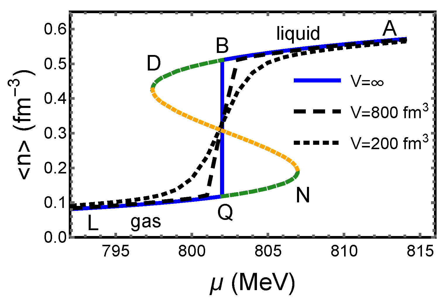
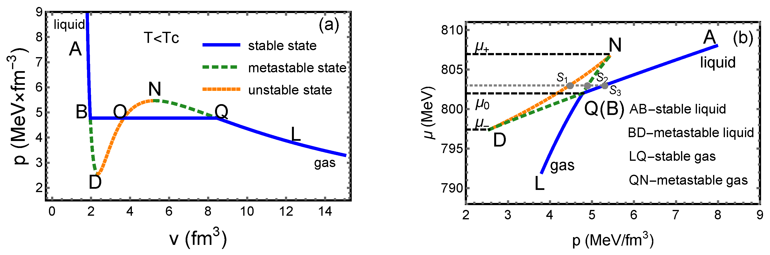
At $T<T_c$, the function $p\left(v\right)$ gives an isotherm, i.e., a spinodal curve, shown in Figure 1a.

On this curve, the segment DON represents an instable state where the condition of stable equilibrium ${\left(\frac{\partial p}{\partial V}\right)}_T<0$ is violated. An orange dotted line is used to denote unstable states in Figure 1a. The conditions of phase equilibrium require that a horizontal line BOQ is constructed to replace the spinodal curve in order to maintain equal T, p and $\mu$ in the two phases (also known as Maxwell’s construction). An equilibrium phase transition between the gas and the liquid takes place along the straight line BOQ rather than the spinodal curve. The systems on segments AB, BOQ and QL correspond to a pure liquid, gas–liquid coexistence and a pure gas, which are all stable states, denoted by blue lines in Figure 1a. The condition of stable equilibrium does not exclude segments BD and NQ. The systems on the two segments are possible to appear but will rapidly evolve to some corresponding states on line BOQ in case of disturbance. That is why they are called metastable states. The metastable states, plotted as green dashed lines in Figure 1a, were confirmed by experiments and named super-heated liquid and super-cooled gas [27], respectively.

Another isotherm can be expressed by $\mu \left(p\right)$. By solving the GCE EoS (2) at given T and $\mu$, particle number density n can be obtained. There are unique or three solutions, denoted by $n_i(T,\mu )$, $i=1$ or $i=1,2,3$. By putting $n_i$ into the variant form of EoS (1), i.e.,

$$\begin{array}{c}\hfill p(T,n)=\frac{nT}{1-bn}-a{n}^2,\end{array}$$

(5)

the pressure $p_i(T,\mu )$ can be obtained, with unique or three values, too. If T is fixed, an isotherm expressed by $\mu \left(p\right)$ is plotted in Figure 1b for $T<T_c$. Using the thermodynamical identity ${\left(\frac{\partial \mu }{\partial p}\right)}_T=v$, one can present the chemical potential ${\mu }_{\mathrm{X}}$ at any point X on the isotherm as

$$\begin{array}{c}\hfill {\mu }_{\mathrm{X}}={\mu }_{\mathrm{Y}}+{\int }_{p_{\mathrm{Y}}}^{p_{\mathrm{X}}}\mathrm{d}{p}^{\prime }v(p^{\prime },T),\end{array}$$

(6)

where the integration is performed along the isotherm from point Y to point X. According to Equation (6), the chemical potential decreases with v if ${\left(\frac{\partial p}{\partial v}\right)}_T<0$, and it increases if ${\left(\frac{\partial p}{\partial v}\right)}_T>0$. Therefore, the chemical potential is a monotonously decreasing function of v along ABD (in Figure 1a) and reaches its minimal value at D. Then, it increases along DON and reaches its maximal value at N. Next, the chemical potential decreases monotonously along NQL. Therefore, segment ABD in Figure 1b is the liquid state, with AB denoting a stable liquid (blue line) and BD denoting a metastable liquid (green dashed line); segment NQL is the gas state, with LQ denoting a stable gas (blue line) and QN denoting a metastable gas (green dashed line); and the coexistence line BOQ in Figure 1a changes to a point Q(B) in Figure 1b.

The chemical potential of the first-order phase transition is denoted as ${\mu }_0$, i.e., the value at point Q(B) in Figure 1b. ${\mu }_{-}$ denotes the chemical potential of point D and ${\mu }_{+}$ denotes that of point N. As the green dashed lines indicate, metastable states are possible to appear in the interval $\mu \in ({\mu }_{-},{\mu }_{+})$. At another temperature, a similar $\mu \left(p\right)$ plot can be obtained, as long as $T<T_c$, giving another set of ${\mu }_0$, ${\mu }_{-}$ and ${\mu }_{+}$. 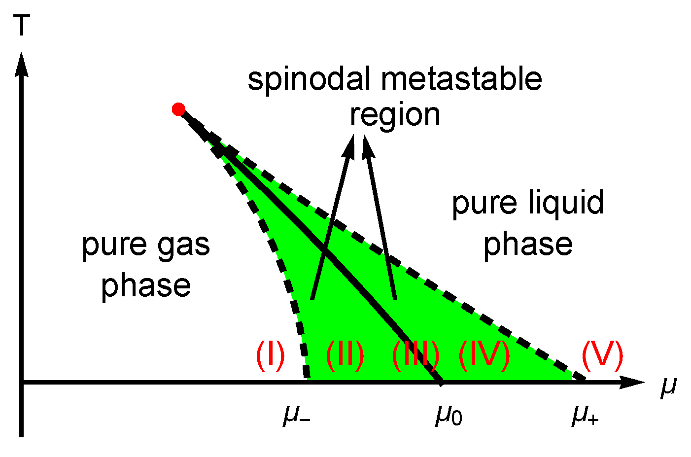By such procedure, we obtain the three curves ${\mu }_0\left(T\right)$, ${\mu }_{-}\left(T\right)$ and ${\mu }_{+}\left(T\right)$, as plotted in Figure 2.

${\mu }_0\left(T\right)$, denoted by the solid line in Figure 2, is just the well-known gas–liquid coexistence line, which forms the boundary of gas phase and liquid phase, in the sense of the thermodynamic limit. In Figure 2, the red point denotes the critical point. The region between ${\mu }_{-}$ and ${\mu }_{+}$ is colored in green, demonstrating the spinodal metastable region where both the stable states and the metastable states are possible states. Thus, the phase diagram is divided into five regions, which are marked by Roman numerals I-V in Figure 2. Region I ($\mu <{\mu }_{-}$) describes a pure gas; Region II (${\mu }_{-}<\mu <{\mu }_0$) describes the spinodal region of a stable gas (corresponding to segment LQ in Figure 1b) and a metastable liquid (corresponding to segment BD in Figure 1b); Region III ($\mu ={\mu }_0$) describes the coexistence of the gas and the liquid; Region IV (${\mu }_0<\mu <{\mu }_{+}$) describes the spinodal region of a metastable gas (see segment QN) and a stable liquid (see segment AB); Region V ($\mu >{\mu }_{+}$) describes a pure liquid. Both Region II and Region IV are spinodal metastable regions.

In the thermodynamic limit, only the stable states are adopted due to the criteria of stable equilibrium. As Figure 1b shows, in order to choose the stable state, the criteria of the minimum chemical potential at a fixed pressure is equivalent to the criteria of the maximum pressure at a fixed chemical potential. For example, at a given temperature and chemical potential, there are three solutions of Equation (2) in the case of ${\mu }_{-}<\mu <{\mu }_0$ or ${\mu }_0<\mu <{\mu }_{+}$. The three solutions are located on the orange, green and blue lines, respectively, as points $s_1$, $s_2$ and $s_3$ in Figure 1b show. The solution $s_3$ on the blue line is chosen due to its maximum pressure. That means the metastable states $s_2$ do not play a role in the thermodynamic limit. However, in the case of finite volume, metastable states play an important role in the spinodal metastable region, as will be illustrated below.

3.2. The Probability of the Metastable State and Its Dependence on the Volume

Let us show the metastable state in the distribution of the particle number density of the van der Waals fluid and its role in understanding the finite-volume effects. According to the standard formula in statistical physics, the probability for a system with particle number N in the grand canonical ensemble is as follows,

$$P\left(N\right)\equiv P(N;V,T,\mu )=\frac{{\left(e^{\frac{\mu }{T}}\right)}^N{\mathcal{Z}}_{\mathrm{CE}}^{\mathrm{vdW}}(V,T,N)}{{\sum }_N{\left(e^{\frac{\mu }{T}}\right)}^N{\mathcal{Z}}_{\mathrm{CE}}^{\mathrm{vdW}}(V,T,N)},$$

(7)

where the partition function of the van der Waals fluid in the canonical ensemble is given in Equation (A7). Based on $P\left(N\right)$, the distribution of the number density $P\left(n\right)$ can also be obtained, which is volume dependent.

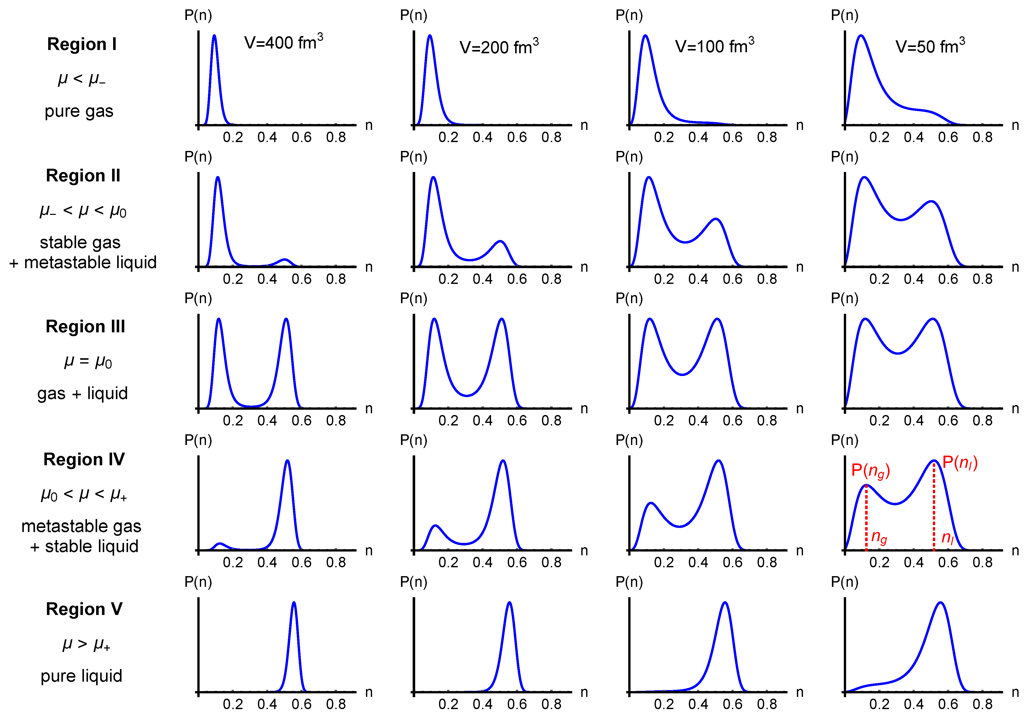
Figure 3 shows the distribution of the number density $P\left(n\right)$ in the five regions of the phase diagram.We see double-peak shapes in Regions II, III and IV. In Region III, the two peaks are always of equal height. In Region II, the left peak is dominant, while in Region IV, the right peak is dominant. Four finite volumes are studied in Figure 3. In Regions II and IV, the relative height of the two peaks varies with volume.

The double-peak shape of the distribution is due to a convex anomaly in entropy or free energy [22]. According to the Landau–Ginzburg theory, the free energy has two valleys for $T<T_c$, which results in two peaks in the distribution of the order parameter according to the relation $P\left(X\right)\sim exp(-F)$ [27]. Therefore, the first-order phase transition of finite volume is associated with a double-peak distribution of the order parameter. On the phase boundary, the two peaks are of equal height, while nearby the phase boundary, the two peaks are of different height.

In order to understand the physical meaning of each peak in Figure 3, we give an example in

Table 1. The solutions of Equation (2) at $T=62$ MeV and $\mu =803$ MeV. The three solutions correspond to the three points $s_{1,2,3}$ in Figure 1b.

n (fm${}^{-3}$)	p (MeV· fm${}^{-3}$)
$n_1$ = 0.290612	$p_1$ = 4.47057	instable
$n_2$ = 0.124643	$p_2$ = 4.89833	metastable gas ($n_g=n_2$)
$n_3$ = 0.518450	$p_3$ = 5.29507	stable liquid ($n_l=n_3$)

. For $T=62$ MeV and $\mu =803$ MeV (a randomly chosen point in Region IV), the solutions of Equation (2) are shown in the first column of Table 1. Putting $n_i(i=1,2,3)$ and $T=62$ MeV into Equation (5), the corresponding pressure is obtained and shown in the second column of Table 1. A horizontal gray dotted line of $\mu =803$ MeV is plotted in Figure 1b, showing three intersections with the isotherm. Point $s_1$ (corresponding to the solution of $n_1$) is located on the orange dotted line, so $n_1$ is instable; point $s_2$ (corresponding to the solution of $n_2$) is located on the green dashed line QN, so $n_2$ denotes a metastable gas, i.e., $n_g=n_2=0.124643$ fm${}^{-3}$; $s_3$ (corresponding to the solution $n_3$) is located on the blue line AB, so $n_3$ denotes a stable liquid, i.e., $n_l=n_3=0.518450$ fm${}^{-3}$. The two data of $n_g=0.124643$ fm${}^{-3}$ and $n_l=0.518450$ fm${}^{-3}$ are drawn as the red dotted lines on one of the distribution plots in Figure 3, which correspond to the maximum of the distribution. The left peak describes the gas, and the right peak describes the liquid. Moreover, the higher peak describes the stable state, and the lower peak describes the metastable state.

When $\mu$ varies from Region I to Region V, the two peaks compete against each other (see from top to bottom in the same column in Figure 3). The unique peaks at Region I and Region V represent a pure gas state and a pure liquid state, respectively. Near the phase boundary, both the gas and the liquid are possible states in the ensemble. The only difference lies in their probabilities of occurrence. On one side of the phase boundary, only one phase is dominant. From Region II to Region IV, the system evolves from a gas-dominant state to a liquid-dominant state.

What do we mean by saying a gas-dominant state nearby the phase boundary? Take the time evolution of the magnetization M in the Monte Carlo simulation of the Ising model below $T_c$ as an example [28]. When on the phase boundary, i.e., the external field $H=0$, the magnetization M shows many transitions between $+M_L$ and $-M_L$. $M=\pm M_L$ represents two ordered phases, i.e., the upward magnetization and downward magnetization. The time lengths staying at $+M_L$ and $-M_L$ are almost equal. When below the phase boundary, i.e., H obtains a small negative value, M shows transitions between $+M_L$ and $-M_L$ too, with a longer time (larger probability) staying at $-M_L$. If there are many replicas of the system in an ensemble (like the samples obtained by the Monte Carlo simulations), some systems are in the phase of upward magnetization and others are in the phase of downward magnetization. The number of systems of the downward magnetization is more than that of the upward magnetization. That represents a downward magnetization-dominant state. Therefore, a gas-dominant state represents an ensemble where the number of systems staying in a gas state is more than that of liquid.

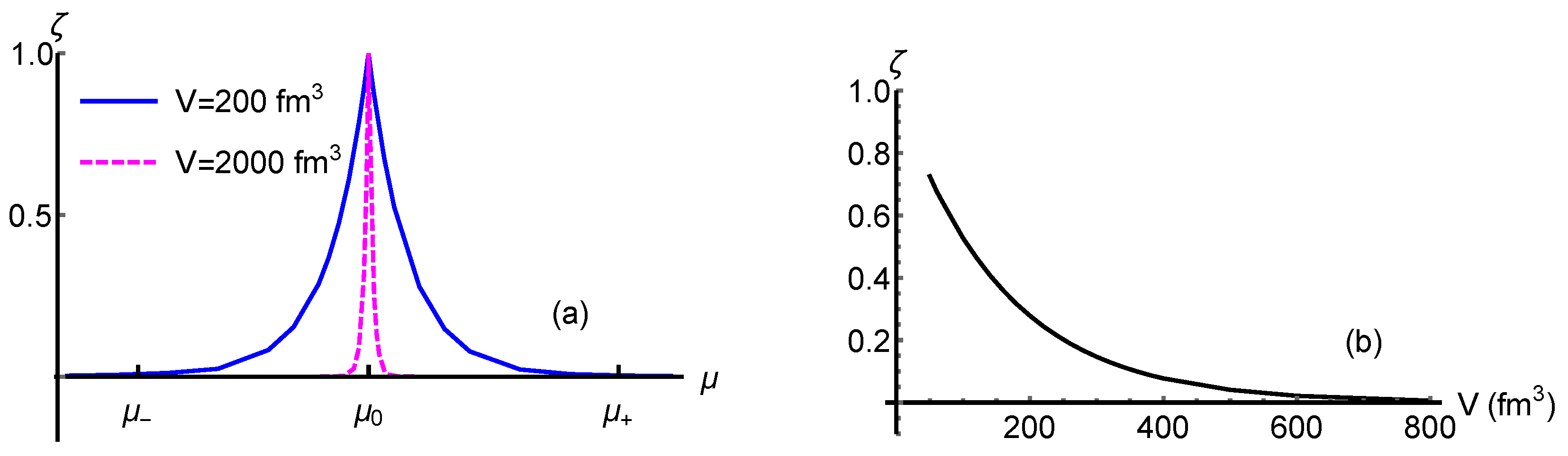
It is widely known that the phase boundary is well-defined in the thermodynamical limit. However, in the case of finite volume, there can not be a clear boundary. Within the spinodal metastable region, both phases are possible to appear. To quantify the relative probability of the metastable state, we define

$$\zeta \equiv \frac{P_{\mathrm{MS}}}{P_{\mathrm{SS}}},$$

(8)

where $P_{\mathrm{MS}}$ and $P_{\mathrm{SS}}$ are the probability peak heights of the metastable state and the stable state, respectively.

The chemical potential dependence of $\zeta$ at a fixed volume, e.g., $V=200$ fm${}^3$, is shown as the blue curve in Figure 4a. $\zeta$ equals to 1 at ${\mu }_0$ and gradually decreases to 0 at both sides. The non-zero relative probability illustrates the contribution of metastable states at a finite volume.

As the volume increases to 2000 fm${}^3$, the area enclosed by the purple curve shrinks and $\zeta$ decreases to 0 more rapidly. That means a metastable state can be observed within a narrower $\mu$ interval. We can expect that the interval of the chemical potential will shrink to zero as the volume approaches infinity. That confirms the statement that metastable states do not have a role to play in the thermodynamic limit.

The spinodal metastable region in the last subsection is specified by the interval $({\mu }_{-},{\mu }_{+})$ for systems with a varying particle number. According to Figure 4a, we can infer that the size of the metastable region is volume dependent for finite-size systems. The smaller the volume, the larger the metastable region.

To quantify how the relative height of the two peaks varies with the volume, $\zeta$ as a function of volume is shown in Figure 4b. It approximately has a law of

$$\zeta \sim exp(-V),$$

(9)

which is consistent with the Ising model [28].

3.3. Metastable States’ Contribution in Understanding Finite-Size Effects of the First-Order Phase Transition

The number density n, as an order parameter of van der Waals fluid, is shown in Figure 5. A spinodal curve ABDNQL is obtained by solving Equation (2) for $T<T_c$. Same as the previous designation, the blue solid line, the green dashed line and the orange dotted line represent stable states, metastable states and instable states, respectively. Because the criteria of a stable equilibrium only chooses stable states, the order parameter n shows the discontinuity in the thermodynamical limit, as the blue line shows in Figure 5.

The number density at finite volume is calculated by obtaining the average from the distribution $P\left(n\right)$. The discontinuity of the number density is rounded at finite volumes, as the black dashed line and black dotted line show in Figure 5. The width $\Delta \mu$ over which the transition is rounded is approximately inversely proportional to the volume, i.e.,

$$\Delta \mu \propto \frac{1}{V}=\frac{1}{L^d},$$

(10)

where d is the dimension of the system. This relation is in agreement with the Ising model [28] and the finite-size scaling theory [29,30,31,32].

When $\mu <{\mu }_0$, the ensemble is a gas-dominant state. In this state, the relative probability of the metastable liquid is $\zeta$ and the average number density can be approximately related to $\zeta$ as a weighted average,

$$\begin{array}{c}\hfill {\langle n\rangle }_V\simeq \frac{n_g+\zeta n_l}{1+\zeta }.\end{array}$$

(11)

Because $\zeta$ is volume-dependent, the average number density is also volume-dependent and can be labeled by a subscript V. Due to $n_g<n_l$, the contribution of the metastable liquid results in ${\langle n\rangle }_V>n_g$ for $\mu <{\mu }_0$. That explains that the black curves representing two finite volumes are above the blue curve at the left of the discontinuity point. In particular, due to ${\zeta |}_{V=200}{>\zeta |}_{V=800}$ (see the left half of Figure 4a), there is ${\langle n\rangle }_{V=200}>{\langle n\rangle }_{V=800}$ for $\mu <{\mu }_0$. That is the reason why the dotted line (for 200 fm${}^3$) is higher than the dashed line (for 800 fm${}^3$) at the left neighborhood of the discontinuity. Therefore, the volume ordering of the number density at finite volumes reflects the contributions of the metastable states. The smaller the volume, the larger the relative probability of the metastable state, and the smoother and flatter the curve of the number density.

When the chemical potential approaches the discontinuity point ${\mu }_0$, $\zeta$ approaches 1 for whatever volume, as Figure 4a shows. It results in

$${\langle n\rangle }_V{|}_{{\mu }_0}\simeq \frac{n_l+n_g}{2},\mathrm{independent}\mathrm{of}\mathrm{volume},$$

(12)

which generates the fixed point behavior (the intersection point of curves of different volumes).

3.4. A Possible Metastable State in the STAR Data at 7.7 GeV

The conjectured QCD phase diagram has the same structure as that of the van der Waals fluid. The lattice QCD and NJL models predict that high cumulants of conserved charges are sensitive observables of the critical point [16,17,18]. The conserved charges, especially the number density of net baryon, denoted as $n_{\mathrm{netB}}$, plays the role of the order parameter of the QCD phase transition. It obtains a small value in the hadronic phase and a large value in the quark phase, i.e., $n_{\mathrm{netB}}^{\mathrm{hadron}}<n_{\mathrm{netB}}^{\mathrm{quark}}$ [33] (the quark number density shown in Reference [33] is just the baryon number density except a factor of $1/3$). Because the freeze-out line is located in the hadronic phase, if it is close to the first-order phase transition line, we hope to see a lower peak on the right side of the distribution representing the metastable quark phase.

In Reference [23], a two-component model was constructed to reproduce the first four factorial cumulants of the proton at 7.7 GeV, especially to explain the large four-particle correlations. If there are two different types of events, denoted by (a) and (b), the distribution of N (the number of proton) is given by

$$P\left(N\right)=(1-\alpha )P_{\left(\mathrm{a}\right)}\left(N\right)+\alpha P_{\left(\mathrm{b}\right)}\left(N\right),$$

(13)

where $(1-\alpha )$ and $\alpha$ denote the probability that an event belongs to class (a) and (b). $P_{\left(\mathrm{a}\right)}\left(N\right)$ and $P_{\left(\mathrm{b}\right)}\left(N\right)$ are multiplicity distributions governing the event classes (a) and (b), respectively. The factorial cumulants (the relation between the cumulants and the factorial cumulants is discussed in Reference [34]) of the total distribution read

$$\begin{array}{ccc}\hfill \langle N\rangle & =& (1-\alpha )\langle N_{\left(\mathrm{a}\right)}\rangle +\alpha \langle N_{\left(\mathrm{b}\right)}\rangle ,\hfill \\ \hfill C_2& =& C_2^{\left(\mathrm{a}\right)}-\alpha ({\overline{C}}_2-(1-\alpha ){\overline{N}}^2),\hfill \\ \hfill C_3& =& C_3^{\left(\mathrm{a}\right)}-\alpha \{{\overline{C}}_3+(1-\alpha )[(1-2\alpha ){\overline{N}}^3-3\overline{N}{\overline{C}}_2]\},\hfill \\ \hfill C_4& =& C_4^{\left(\mathrm{a}\right)}-\alpha \{{\overline{C}}_4-(1-\alpha )[(1-6\alpha +6{\alpha }^2){\overline{N}}^4\hfill \\ & -& 6(1-2\alpha ){\overline{N}}^2{\overline{C}}_2+4\overline{N}{\overline{C}}_3+3{\left({\overline{C}}_2\right)}^2\left]\right\},\hfill \end{array}$$

(14)

where

$$\begin{array}{ccc}\hfill \overline{N}& =& \langle N_{\left(\mathrm{a}\right)}\rangle -\langle N_{\left(\mathrm{b}\right)}\rangle ,\hfill \\ \hfill {\overline{C}}_n& =& C_n^{\left(a\right)}-C_n^{\left(b\right)},\hfill \end{array}$$

(15)

and $C_n^{(a/b)}$ represents the factorial cumulants of the class (a) or (b).

The factorial cumulants of the model are given in Equation (14). The mean value of the first four factorial cumulants in the STAR Au+Au collision data at 7.7 GeV are as follows [20,23],

$$\begin{array}{ccc}\hfill \langle N\rangle & =& 39.2908,C_2=-1.7511,\hfill \\ \hfill C_3& =& -10.3098,C_4=172.906.\hfill \end{array}$$

(16)

A combination of a binomial distribution (event classes (a)) and a Poisson distribution (event classes (b)) are used in Reference [23]. There are four parameters in total, including two parameters from the binomial distribution, one parameter from the Poisson distribution and one weight factor $\alpha$. One of the parameters in the binomial distribution is fixed and they only fit $\langle N\rangle$, $C_3$ and $C_4$. In this section, we follow the method in Reference [23], but fit all the first four factorial cumulants, without fixing any parameters. 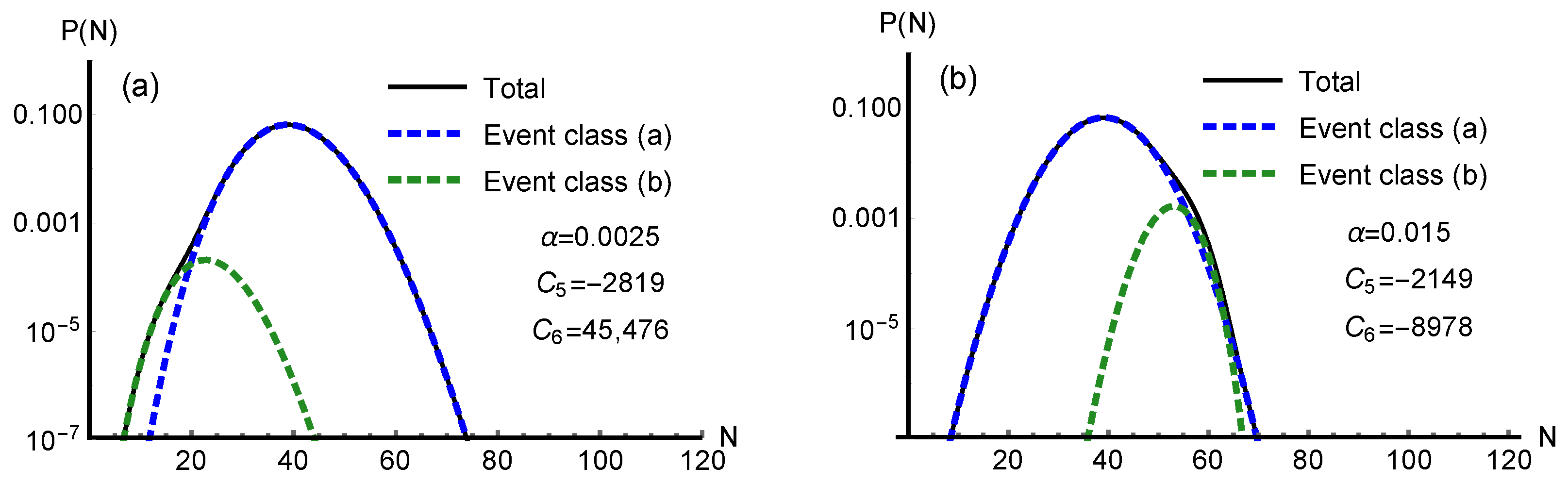Each formula in Equation (14) should be equal to the corresponding mean value given in Equation (16), forming four equations. Since the number of parameters is equal to the number of equations, the parameters are exactly determined by solving the set of equations. The result is shown in Figure 6a. The distribution indeed shows a two-peak shape.

However, it does not agree with the prediction from the metastable state. Because the number of anti-baryon is much less than that of baryon at low-energy collisions, we expect the number of baryon can approximate the number of net baryon. Thus, $n_{\mathrm{B}}^{\mathrm{hadron}}<n_{\mathrm{B}}^{\mathrm{quark}}$ should hold and $n_{\mathrm{proton}}^{\mathrm{hadron}}<n_{\mathrm{proton}}^{\mathrm{quark}}$ approximately holds. In the case of a first-order phase transition, the lower peak of the metastable state representing the quark phase should be located on the right side. Figure 6a does not show this feature.

In fact, there is not a unique way to identify the distribution in only reproducing the first four factorial cumulants. We try some other fittings and find that a combination of a normal distribution (event class (a)) and a binomial distribution (event class (b)) can also reproduce the first four factorial cumulants measured by STAR, which is shown in Figure 6b. There are five parameters in total, including two parameters from a normal distribution, two from a binomial distribution and one weight factor $\alpha$. Fitting only four factorial cumulants needs to fix one parameter. Here, we fix the integer parameter of the binomial distribution to be 70. In this case, the lower peak representing the metastable quark phase lies on the right side as the green dashed line in Figure 6b shows, being consistent with the scenario of the first-order phase transition. So far, the physical meaning of the two components becomes clear. They represent two phases. The dominant component (event class (a)) represents the stable phase, and the small component (event class (b)) represents the metastable phase. The presence of the metastable phase may signal a first-order phase transition.

Even though the weight factor $\alpha$ is small ($\alpha =$ 0.0025 and 0.015 in Figure 6a,b, respectively), the small component can not be ignored. Without the contribution of the small component, the four factorial cumulants can not be well reproduced. Particularly, the small component has a vital effect on higher cumulants, such as $C_6$. As the legends show, $C_6$ = 45,476 and $-8978$ in Figure 6a,b, respectively. That means, even though the first four factorial cumulants are equal by magnitude for both cases, the fifth factorial cumulant differs by $\sim 30\%$ and the sixth factorial cumulant differs significantly (by 5 times in magnitude as well as a different sign).

In case the lower peak in Figure 6b is a metastable quark phase, the extremely small weight factor $\alpha$ (reflecting a small relative probability of the metastable state) may hint that the freeze-out point is a little far from the first-order phase transition line. In addition, the two peaks are not separated far enough in the current data. If the collision energy decreases, the temperature decreases and the difference between $n_{\mathrm{proton}}^{\mathrm{hadron}}$ and $n_{\mathrm{proton}}^{\mathrm{quark}}$ increases. The centers of the two peaks will be further apart and it will be better to observe the double-peak structure.

Whether the metastable state is spotted strongly depends on the upcoming measurements of higher factorial cumulants, especially $C_6$. As indicated in Figure 6, $C_5$ has the same sign and a similar figure in both cases, while $C_6$ has an opposite sign and differs much. A definite conclusion should be drawn on the basis of the future $C_6$ measurement.

4. Summary and Conclusions

In this paper, we revisit the van der Waals fluid and map the spinodal metastable region in the phase diagram. It is a triangular band along the first-order transition line. In the thermodynamic limit, the first-order phase transition line serves as a boundary between the gas and the liquid. However, at a finite volume, the phase boundary loses its original meaning and is replaced by a triangular band where both phases are possible states.

Finite volumes make the metastable state visible in the distribution of the order parameter. On the phase boundary, the distribution has two peaks of equal height. Near the phase boundary, the distribution is still a two-peak shape, but their heights are unequal. The origin of the two-peak distribution is a convex anomaly in the entropy or free energy. The two valleys of free energy at $T<T_c$, as the Landau–Ginzburg theory shows, generate the two peaks of the distribution of the order parameter. The two peaks represent two phases. The higher peak represents the stable state, while the lower peak represents the metastable state. The probabilities of the metastable state are less than that of the stable state. At the left half of the green area in Figure 2, the gas phase is the stable state and its probability in the ensemble is dominant, while the liquid phase is the metastable state and its probability is less prominent. The dominant peak at one side of the phase boundary becomes less dominant at the other side.

The relative probability of the metastable state $\zeta$ has significant volume dependence. The rule that the probability $\zeta$ decreases exponentially with the volume is consistent with the Ising model. At the same T and $\mu$, the smaller the volume, the larger the probability of the metastable state. As a result, the size of the metastable region is also volume dependent. The smaller the volume, the larger the metastable region in the phase diagram. At a given volume, the closer to the phase boundary, the easier it is to find the metastable state. The metastable states play important roles in understanding the finite-size effects of the first-order phase transition. The smoothness of the discontinuity of the order parameter at finite volume reflects the contribution of the metastable states. The volume ordering, even the fixed point, of the number density can also be understood by considering the contribution of the metastable states.

By fitting the first four factorial cumulants of the proton number in the STAR data at 7.7 GeV, a two-peak distribution, which is consistent with the scenario of the metastable state, is obtained. The presence of a metastable quark phase may hint at a first-order phase transition. However, the statement is still uncertain. Due to the non-uniqueness of the fitting, future measurements of higher factorial cumulants, e.g., $C_6$, will help to distinguish the scenarios. The fitting made in this study may indicate that the freeze-out point of 7.7 GeV is within the spinodal metastable region. There are two suggestions according to this study. First, the current weight factor $\alpha$ (reflecting the probability of the metastable state) is rather small. To enhance the probability of the metastable state, a smaller system size is favored. Second, the centers of the current two peaks are not separated far enough. A lower collision energy is favored to decrease the temperature. Then, the two peaks will be further apart and easier to observe.

References

1. Lee, T.D.; Wick, G.C. Vacuum stability and vacuum excitation in a spin-0 field theory. Phys. Rev. D 1974, 9, 2291. [Google Scholar] [CrossRef]
2. Lee, T.D. Abnormal nuclear states and vacuum excitation. Rev. Mod. Phys. 1975, 47, 267. [Google Scholar] [CrossRef]
3. Collins, J.C.; Perry, M.J. Superdense matter: Neutrons or asymptotically free quarks? Phys. Rev. Lett. 1975, 34, 1353. [Google Scholar] [CrossRef]
4. Shuryak, E.V. Quark-gluon plasma and hadronic production of leptons, photons and psions. Phys. Lett. B 1978, 78, 150. [Google Scholar] [CrossRef]
5. Arsene, I.; Bearden, I.G.; Beavis, D.; Besliu, C.; Budick, B.; Bøggild, H.; Chasman, C.; Christensen, C.H.; Christiansen, P.; Cibor, J.; et al. Quark-gluon plasma and color glass condensate at RHIC? The perspective from the BRAHMS experiment. Nucl. Phys. A 2005, 757, 1–27. [Google Scholar] [CrossRef]
6. Back, B.B. (PHOBOS Collab.). The PHOBOS perspective on discoveries at RHIC. Nucl. Phys. A 2005, 757, 28–101. [Google Scholar] [CrossRef]
7. Adams, J.; Aggarwal, M.M.; Ahammed, Z.; Amonett, J.; Anderson, B.D.; Arkhipkin, D.; Averichev, G.S.; Badyal, S.K.; Bai, Y.; Balewski, J.; et al. Experimental and theoretical challenges in the search for the quark-gluon plasma: The STAR Collaboration’s critical assessment of the evidence from RHIC collisions. Nucl. Phys. A 2005, 757, 102–183. [Google Scholar] [CrossRef]
8. Adcox, K.; Adler, S.S.; Afanasiev, S.; Aidala, C.; Ajitanand, N.N.; Akiba, Y.; Al-Jamel, A.; Alexander, J.; Amirikas, R.; Aoki, K.; et al. Formation of dense partonic matter in relativistic nucleus-nucleus collisions at RHIC: Experimental evaluation by the PHENIX Collaboration. Nucl. Phys. A 2005, 757, 184–283. [Google Scholar] [CrossRef]
9. Pisarski, R.D.; Wilczek, F. Remarks on the chiral phase transition in chromodynamics. Phys. Rev. D 1984, 29, 338. [Google Scholar] [CrossRef]
10. Aoki, Y.; Endrodi, G.; Fodor, Z.; Katz, S.D.; Szabo, K.K. The order of the quantum chromodynamics transition predicted by the standard model of particle physics. Nature 2006, 443, 675–678. [Google Scholar] [CrossRef] [Green Version]
11. Asakawa, M.; Yazaki, K. Chiral restoration at finite density and temperature. Nucl. Phys. A 1989, 504, 668–684. [Google Scholar]
12. Barducci, A.; Casalbuoni, R.; Curtis, S.; Gatto, R.; Pettini, G. Chiral phase transitions in QCD for finite temperature and density. Phys. Rev. D 1990, 41, 1610. [Google Scholar] [CrossRef]
13. Berges, J.; Rajagopal, K. Color superconductivity and chiral symmetry restoration at non-zero baryon density and temperature. Nucl. Phys. B 1999, 538, 215–232. [Google Scholar] [CrossRef]
14. Halasz, M.A.; Jackson, A.D.; Shrock, R.E.; Stephanov, M.A.; Verbaarschot, J.J. Phase diagram of QCD. Phys. Rev. D 1998, 58, 096007. [Google Scholar] [CrossRef]
15. Scavenius, O.; Mocsy, A.; Mishustin, I.N.; Rischke, D.H. Chiral phase transition within effective models with constituent quarks. Phys. Rev. C 2001, 64, 045202. [Google Scholar] [CrossRef]
16. Stephanov, M.A. Non-Gaussian fluctuations near the QCD critical point. Phys. Rev. Lett. 2009, 102, 032301. [Google Scholar] [CrossRef]
17. Ejiri, S.; Karsch, F.; Redlich, K. Hadronic fluctuations at the QCD phase transition. Phys. Lett. B 2006, 633, 275–282. [Google Scholar] [CrossRef]
18. Cheng, M.; Hegde, P.; Jung, C.; Karsch, F.; Kaczmarek, O.; Laermann, E.; Mawhinney, R.D.; Miao, C.; Petreczky, P.; Schmidt, C.; et al. Baryon number, strangeness, and electric charge fluctuations in QCD at high temperature. Phys. Rev. D 2009, 79, 074505. [Google Scholar] [CrossRef]
19. Stephanov, M.A. Sign of Kurtosis near the QCD critical point. Phys. Rev. Lett. 2011, 107, 052301. [Google Scholar] [CrossRef]
20. Luo, X.; Xu, N. Search for the QCD critical point with fluctuations of conserved quantities in relativistic heavy-ion collisions at RHIC: An overview. Nucl. Sci. Tech. 2017, 28, 112. [Google Scholar] [CrossRef]
21. Adamczyk, L.; Adkins, J.K.; Agakishiev, G.; Aggarwal, M.M.; Ahammed, Z.; Alekseev, I.; Alford, J.; Anson, C.D.; Aparin, A.; Arkhipkin, D.; et al. Beam-energy dependence of the directed flow of protons, antiprotons, and pions in Au+Au collisions. Phys. Rev. Lett. 2014, 112, 162301. [Google Scholar] [CrossRef] [PubMed]
22. Chomaz, P.; Colonna, M.; Randrup, J. Nuclear spinodal fragmentation. Phys. Rep. 2004, 389, 263–440. [Google Scholar] [CrossRef]
23. Bzdak, A.; Koch, V.; Oliinychenko, D.; Steinheimer, J. Large proton cumulants from the superposition of ordinary multiplicity distribution. Phys. Rev. C 2018, 98, 054901. [Google Scholar] [CrossRef]
24. Das, S. (for the STAR Collab.). Chemical freeze-out parameters from Au+Au collisions at  s NN = 7.7 , 11.5 and 39 GeV. Proc. DAE Symp. Nucl. Phys. 2011, 56, 982. [Google Scholar]
25. Lacey, R.A. Indications for a critical end point in the phase diagram for hot and dense nuclear matter. Phys. Rev. Lett. 2015, 114, 142301. [Google Scholar] [CrossRef]
26. Vovchenko, V.; Anchishkin, D.V.; Gorenstein, M.I. Particle number fluctuations for the van der Waals equation of state. J. Phys. A Math. Theor. 2015, 48, 305001. [Google Scholar] [CrossRef]
27. Landau, L.D.; Lifshitz, E.M. Statistical Physics (Course of Theoretical Physics, Volume 5); Pergamon Press: Oxford, UK, 1980. [Google Scholar]
28. Binder, K.; Landau, D.P. Finite-size scaling at first-order phase transitions. Phys. Rev. B 1984, 30, 1477. [Google Scholar] [CrossRef]
29. Fisher, M.E.; Berker, A.N. Scaling for first-order phase transitions in thermodynamic and finite systems. Phys. Rev. B 1982, 26, 2507. [Google Scholar] [CrossRef]
30. Binder, K. Theory of first-order phase transitions. Rep. Prog. Phys. 1987, 50, 783. [Google Scholar] [CrossRef]
31. van Leeuwen, J.M.J. Singularities in the critical surface and universality for Ising-like spin systems. Phys. Rev. Lett. 1975, 34, 1056. [Google Scholar] [CrossRef]
32. Nienhuis, B.; Nauenberg, M. First-order phase transitions in renormalization-group theory. Phys. Rev. Lett. 1975, 35, 477. [Google Scholar] [CrossRef]
33. Schaefer, B.J.; Wambach, J. Susceptibilities near the QCD (tri)critical point. Phys. Rev. D 2007, 75, 085015. [Google Scholar] [CrossRef] [Green Version]
34. Kitazawa, M.; Luo, X. Properties and uses of factorial cumulants in relativistic heavy-ion collisions. Phys. Rev. C 2017, 96, 024910. [Google Scholar] [CrossRef] [Green Version]
Figure 1. (a) An isotherm in p ( v ) plot at T = 62 MeV (a randomly chosen temperature for T < T c ). (b) An isotherm in μ ( p ) plot.
Symmetry 15 00510 g001
Figure 2. The phase diagram of a van der Waals fluid. The red point denotes the critical point and the solid line denotes the first-order phase transition line in the thermodynamic limit. Spinodal metastable region is marked by the green shaded area.
Symmetry 15 00510 g002
Figure 3. Distribution of the particle number density in five regions of the phase diagram. Each column has the same volume as indicated at the top. From left to right, the volume is 400, 200, 100 and 50 fm 3 , respectively. The left peak describes the gas, and the right peak describes the liquid. The higher peak describes the stable state, and the lower peak describes the metastable state.
Symmetry 15 00510 g003
Figure 4. (a) The relative probability of the metastable state ζ as a function of μ at two given volumes. (b) ζ as a function of volume at μ = 803 MeV ( μ 0 < μ < μ + ).
Symmetry 15 00510 g004
Figure 5. The average number density n at T < T c .
Symmetry 15 00510 g005
Figure 6. The distribution of the proton number. (a) A two-component distribution with a lower peak on the left side, similar to what is performed in Reference [23]. (b) A two-component distribution with a lower peak on the right side which is consistent with the scenario of the metastable state. The blue line represents the stable hadron phase, while the green line represents the metastable quark phase.
Symmetry 15 00510 g006