
Investigations of Symmetrical Incomplete Information Spreading in the Evidential Reasoning Algorithm and the Evidential Reasoning Rule via Partial Derivative Analysis

Abstract
:1. Introduction
2. The Spreading of Incomplete Information via ER and ER Rule
2.1. The Spreading of Incomplete Information via ER
2.2. The Spreading of Incomplete Information via the ER Rule
3. Contribution Calculation within the Framework of ER and the ER Rule
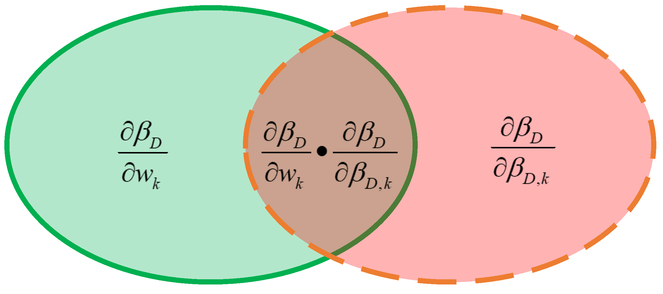
3.1. Contribution Calculation within the Framework of ER
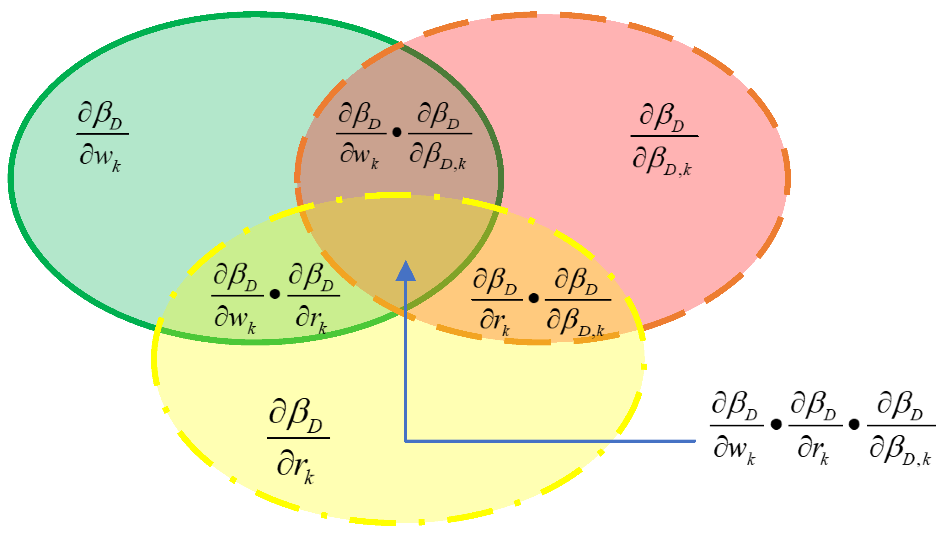
3.2. Contribution Calculation within the Framework of the ER Rule
3.3. Similarities and Dissimilarities between the ER Algorithm and the ER Rule
4. Numerical Case Study
4.1. A Numerical Case via ER: Incomplete Information Calculation
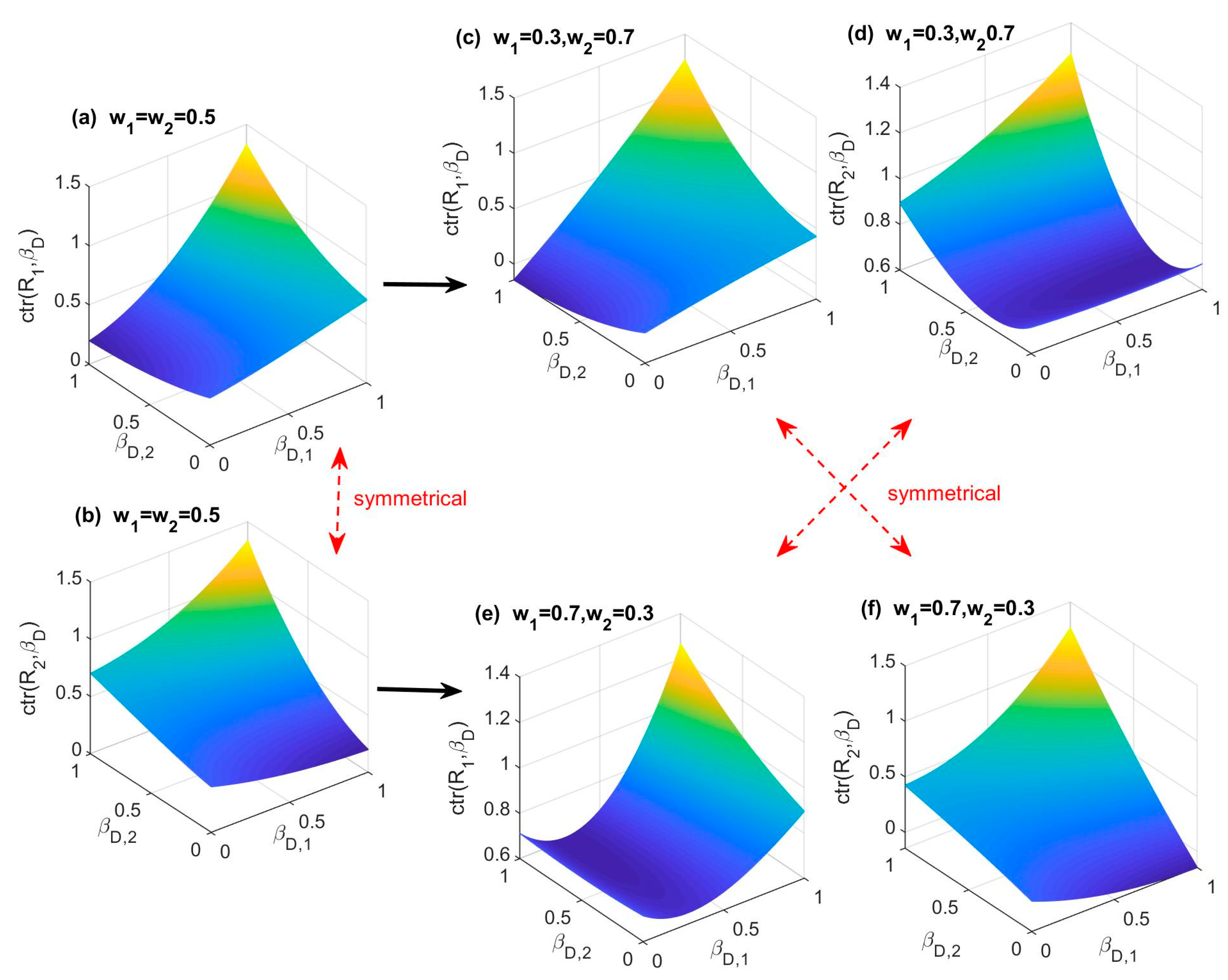
4.2. A Numerical Example via ER: Information Spreading Based on Contribution Calculation
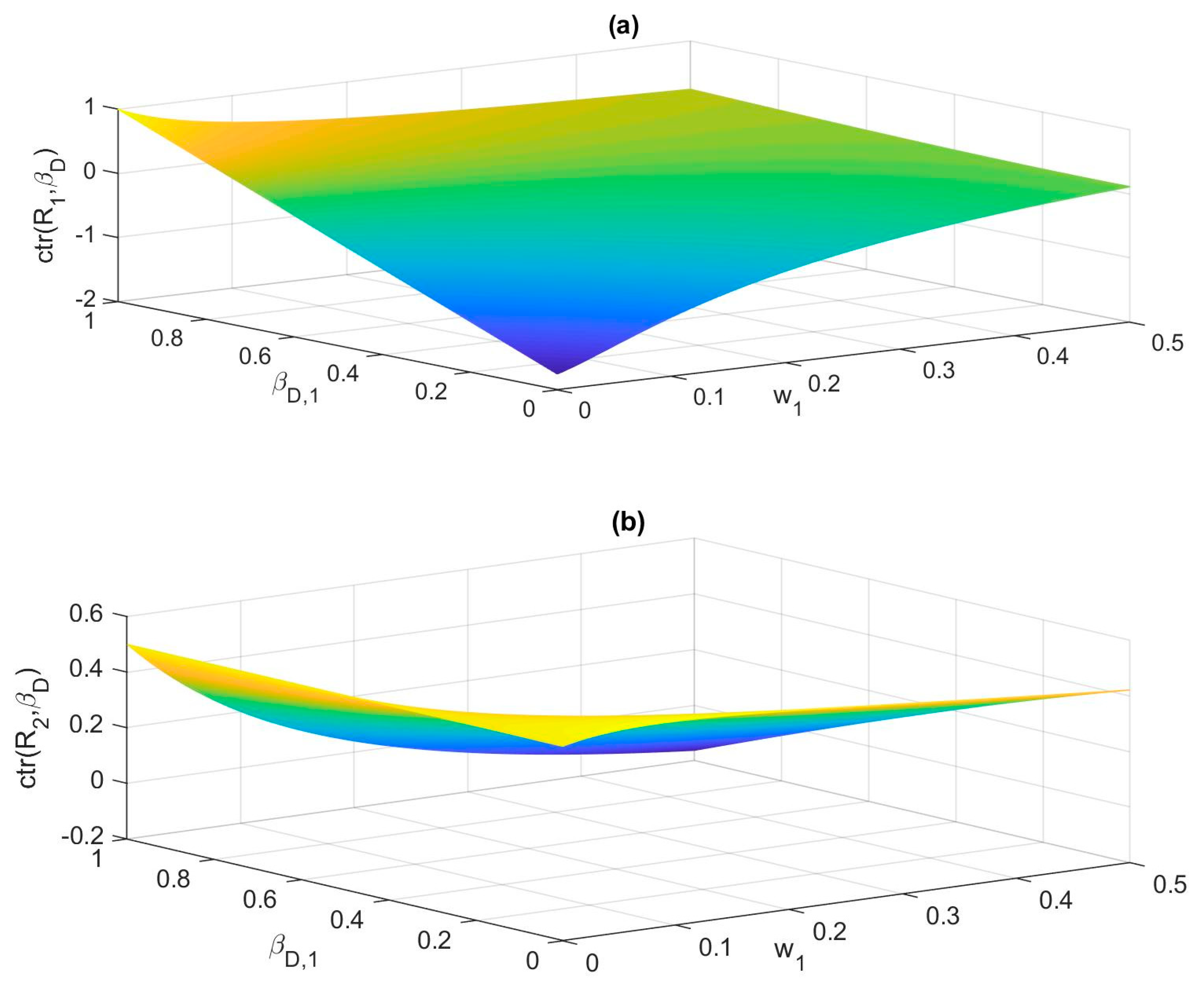
- (1)
- Neither ctr(R1, βD) nor ctr(R2, βD) is symmetrical. Generally, we can observe that the highest contribution is made when βD,1 = 1 and βD,2 = 1, but the lowest contribution is NOT made when βD,1 = 0 and βD,2 = 0. Instead, the contribution reaches the lowest value when βD,1 = 0 and βD,2 = 1, as shown in Figure 4a, and the contribution reaches the lowest value when βD,1 = 1 and βD,2 = 0, as shown in Figure 4b.
- (2)
- Symmetrical results can be observed by comparing Figure 4c,d with Figure 4e,f, i.e., Figure 4c,f and Figure 4d,e are identical. Nonetheless, it can be observed that they both produce tilted images compared with Figure 4a,b. The contribution reaches the lowest value when βD,1 = 0 and βD,2 = 1 (Figure 4c) and when βD,1 = 1 and βD,2 = 0 (Figure 4f). The lowest contribution is not achieved at any endpoint in Figure 4d,f.
- (3)
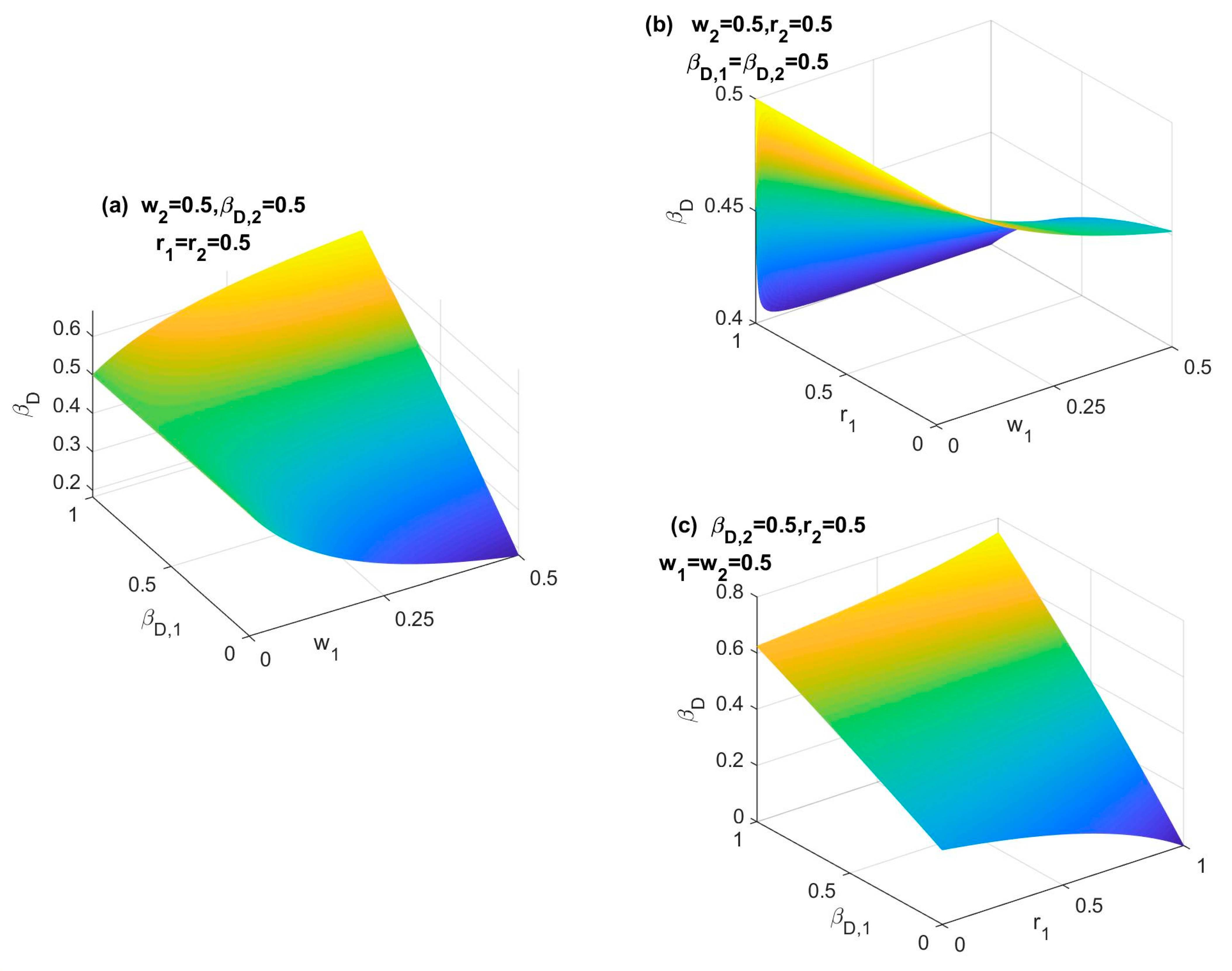
- (1)
- There is an increasing nonlinearity presented in Figure 5a–c. Even in Figure 5a, the nonlinearity is much higher compared with Figure 4a,b. The nonlinearity presented in Figure 5b,c is even higher. Specifically, there is a sharp change in βD when w2→0 and βD,1 = 0.3/βD,2 = 0.7, and also when w1→0 and βD,1 = 0.7/βD,2 = 0.3.
- (2)
- The minimum βD in Figure 5a is obtained while w1 = w2 = 0, and the highest βD is NOT obtained when w1 = w2 = 1, but when w1 = 1 and w2 = 0, or w1 = 0 and w2 = 1, which is beyond the expectation of common understanding. As for when βD,1 = 0.3/βD,2 = 0.7, or βD,1 = 0.7/βD,2 = 0.3, the results are even more unstable, which is consistent with the high nonlinearity, as summarized in (1).
- (3)
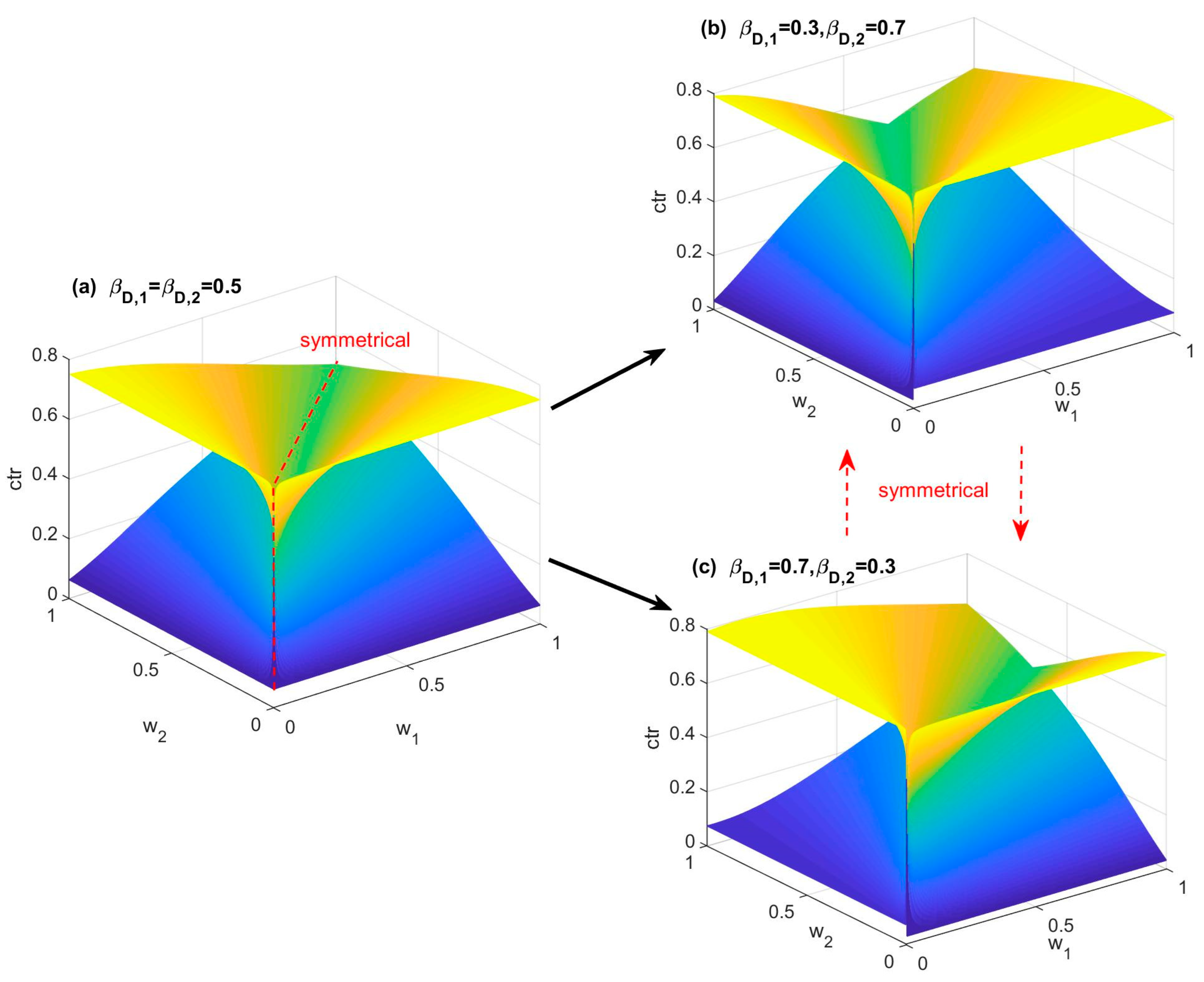
- (1)
- (2)
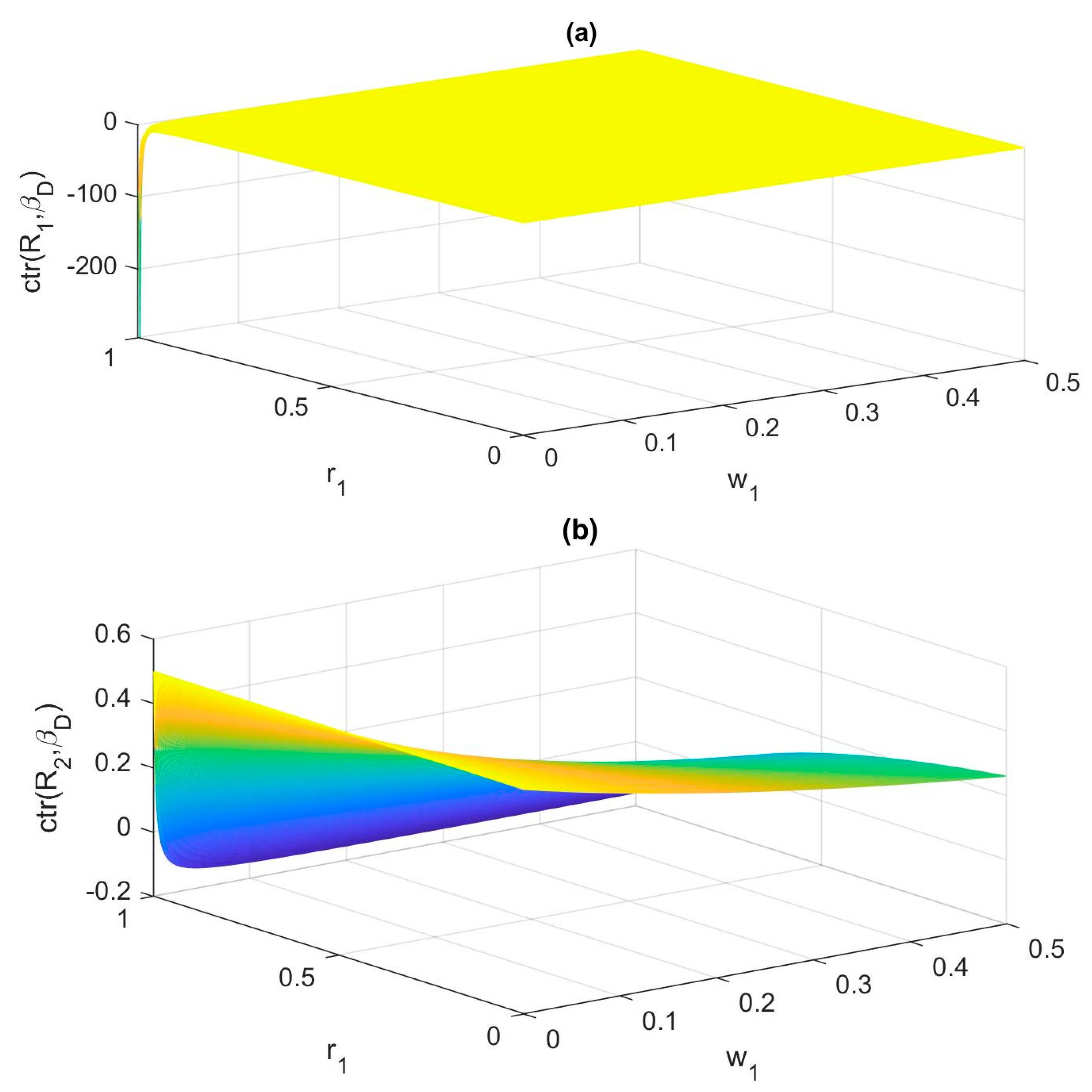
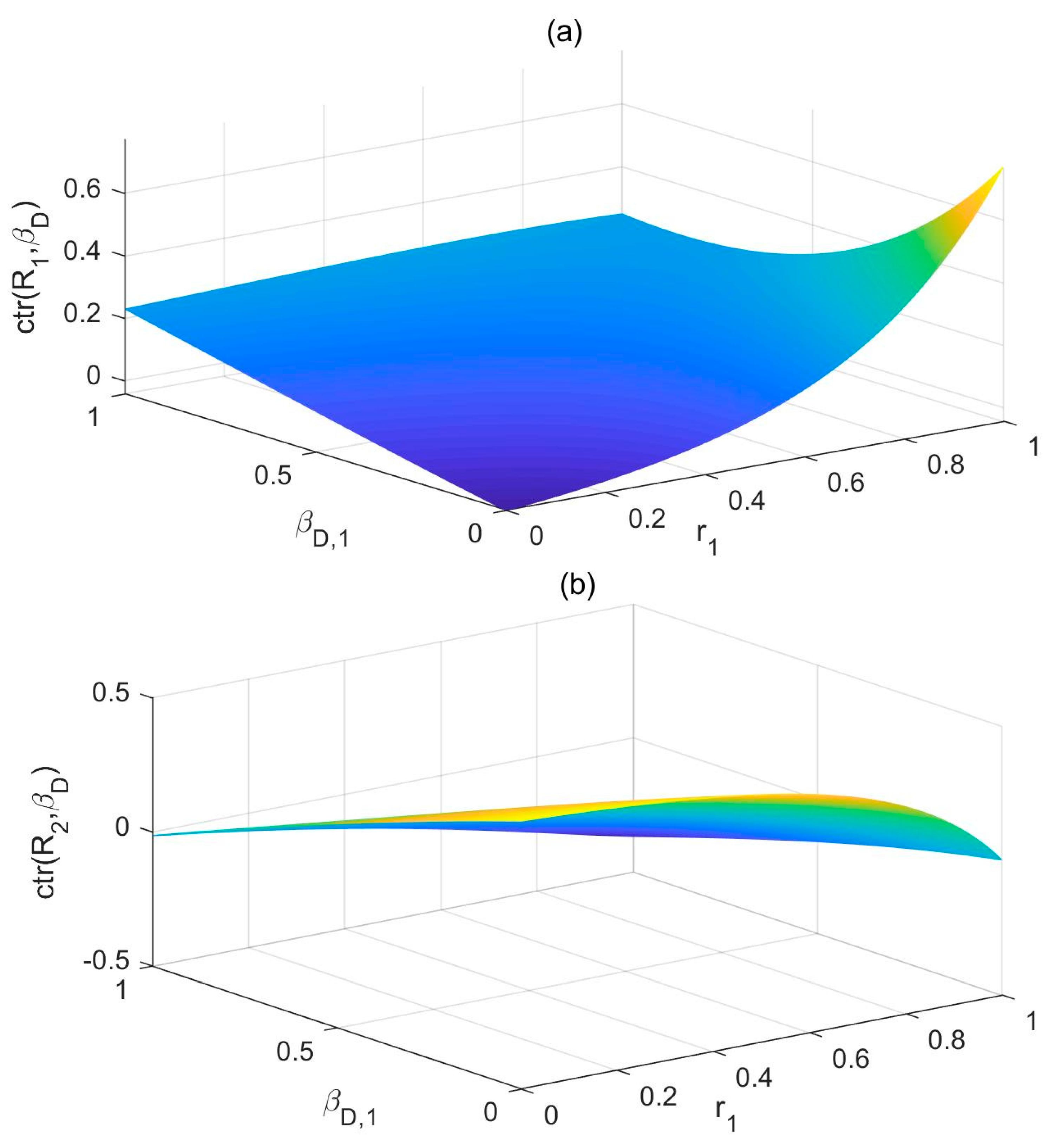
- A high level of symmetry can still be observed in Figure 6a and also in Figure 6b,c. Moreover, there is a certain level of asymmetry within Figure 6b,c. It seems that there is a drastic change in the contribution when βD,1 and βD,2 are imbalanced. Specifically, the image is tilted towards one direction, favoring the rule with a higher βD,k rather than along the axis of w1 = w2.
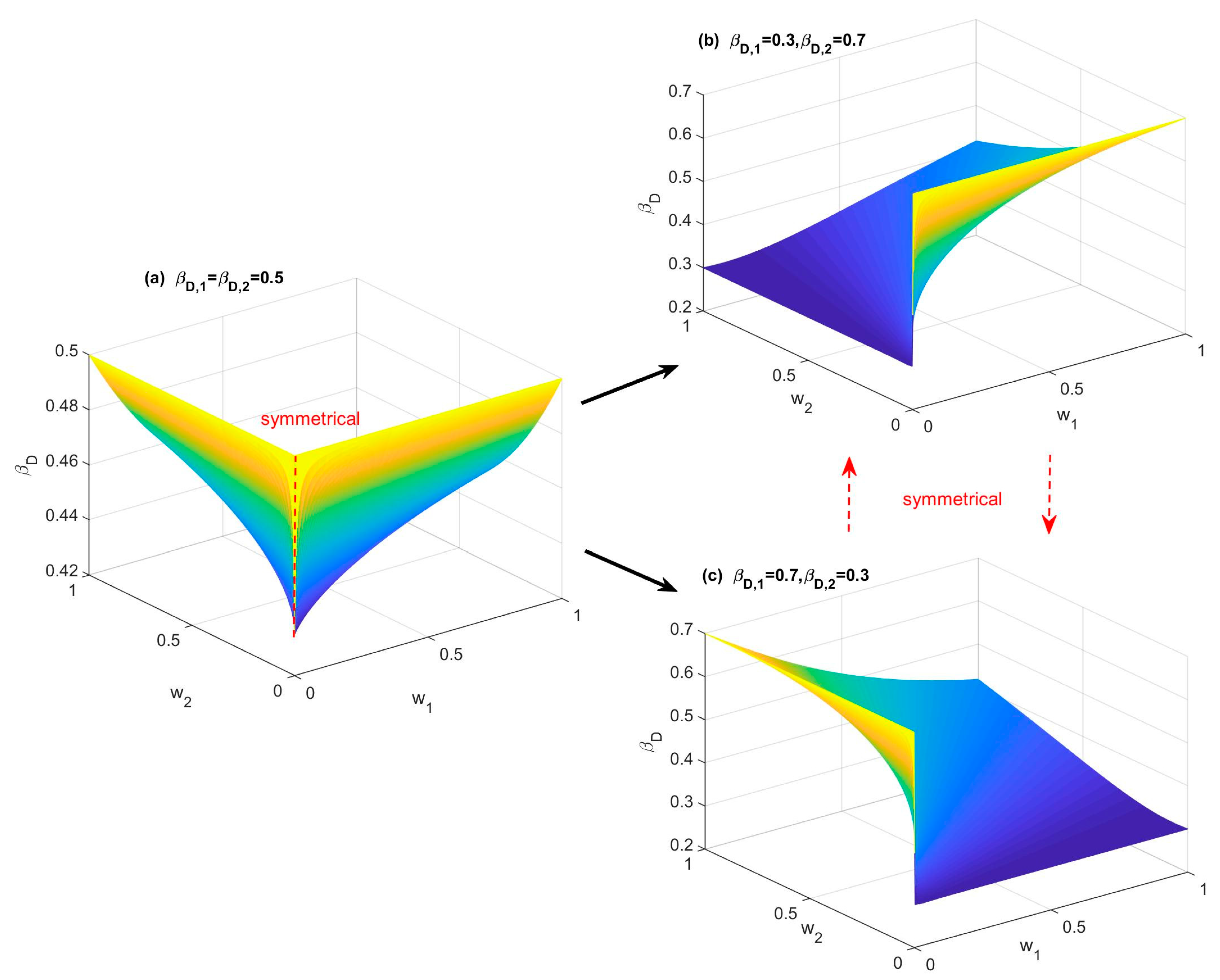
4.3. A Numerical Case via the ER Rule: Incomplete Information Calculation
- (1)
- βD reaches its minimum when βD,1 = 0 and w1 = 0.5, and βD reaches its maximum when βD,1 = 1 and w1 = 0.5.
- (2)
- When w1 is approaching 0, βD is completely determined by βD,2, as it is equal to βD,2, and it does not change along with βD,1. In other words, βD,1 does not contribute βD, and βD = 0.5.
- (3)
- When w1 ≠ 0, βD increases along with the increase in βD,1.
- (4)
- When βD,1 is fixed and below 0.5, βD decreases along with the increase in w1.
- (5)
- When βD,1 is fixed and above 0.5, βD increases along with the increase in w1.
4.4. A Numerical Case via ER Rule: Information Spreading Based on Contribution Calculation
4.5. Summarization
- (1)
- There is a high level of nonlinearity observed both when integrating incomplete information and calculating the contributions made by influential factors. This is mostly owing to the superior nonlinearity modeling ability of the ER algorithm and the ER rule. From a counter perspective, the nonlinearity is expected, as a superior machine learning approach is anticipated to handle the nonlinearity residing in practical problems, or it would be deemed a failed approach.
- (2)
- Symmetry is observed, even when certain parameters are adjusted. This is especially novel in the context of the ER algorithm when the rule reliability is not considered as compared to when the ER rule is considered (in terms of the rule reliability).
- (3)
- Asymmetry is observed, especially concerning the contribution calculation results, and is more novel in the context of the ER rule compared with the ER algorithm. For the ER rule, this is likely because there are three factors, namely the rule reliability, the rule weight, and the incomplete information of the rule. Specifically, there is a higher level of asymmetry and nonlinearity between the rule weight and rule reliability with fixed βD,1 and βD,2.
5. Conclusions
Author Contributions
Funding
Data Availability Statement
Acknowledgments
Conflicts of Interest
References
- Birgitta, D.L.; John, M.W. Human Symmetry Uncertainty Detected by a Self-Organizing Neural Network Map. Symmetry 2021, 13, 299. [Google Scholar]
- Pamitas, S.; Nantana, W.; Sirawadee, A.; Thanawath, N. Resilient supplier selection in electronic components procurement: An integration of evidence theory and rule-based transformation into TOPSIS to tackle uncertain and incomplete information. Symmetry 2020, 12, 1109. [Google Scholar]
- Sun, R.; Yang, Y.; Chiang, K.W.; Duong, T.T.; Lin, K.Y.; Tsai, G.J. Robust IMU/GPS/VO integration for vehicle navigation in GNSS degraded urban areas. IEEE Sens. J. 2020, 20, 10110–10122. [Google Scholar] [CrossRef]
- Neve, B.V.; Schmidt, C.P. Point-of-use hospital inventory management with inaccurate usage capture. Health Care Manag. Sci. 2022, 25, 126–145. [Google Scholar] [CrossRef]
- Horschler, D.J.; Santos, L.R.; MacLean, E.L. Do non-human primates really represent others’ ignorance? A test of the awareness relations hypothesis. Cognition 2019, 190, 72–80. [Google Scholar] [CrossRef]
- Lin, H. Feature Input Symmetry Algorithm of Multi-Modal Natural Language Library Based on BP Neural Network. Symmetry 2019, 11, 341. [Google Scholar] [CrossRef]
- Yang, M.; Li, Y.; Hu, P.; Bai, J.; Lv, J.; Peng, X. Robust multi-view clustering with incomplete information. IEEE Trans. Pattern Anal. Mach. Intell. 2022, 45, 1055–1069. [Google Scholar] [CrossRef]
- Sokat, K.Y.; Dolinskaya, I.S.; Smilowitz, K.; Bank, R. Incomplete information imputation in limited data environments with application to disaster response. Eur. J. Oper. Res. 2018, 269, 466–485. [Google Scholar] [CrossRef]
- Li, Q.; Li, Y.; Liu, S.; Wang, X.; Chaoui, H. Incomplete Information Stochastic Game Theoretic Vulnerability Management for Wide-Area Damping Control Against Cyber Attacks. IEEE J. Emerg. Sel. Top. Circuits Syst. 2022, 12, 124–134. [Google Scholar] [CrossRef]
- Udare, A.; Agarwal, M.; Alabousi, M.; Mclnnes, M.; Rubino, J.G.; Marcaccio, M.; Pol, C.B. Diagnostic Accuracy of MRI for Differentiation of Benign and Malignant Pancreatic Cystic Lesions Compared to CT and Endoscopic Ultrasound: Systematic Review and Meta-analysis. J. Magn. Reson. Imaging 2021, 54, 1126–1137. [Google Scholar] [CrossRef]
- Gassert, F.; Schnitzer, M.; Kim, S.H.; Kunz, W.G.; Ernst, B.P.; Clevert, D.A.; Dominik, N.; Johannes, R.; Froelich, M.F. Comparison of magnetic resonance imaging and contrast-enhanced ultrasound as diagnostic options for unclear cystic renal lesions: A cost-effectiveness analysis. Ultraschall Med.-Eur. J. Ultrasound 2021, 42, 411–417. [Google Scholar] [CrossRef] [PubMed]
- Bi, A.; Ying, W.; Qian, Z. Spatial fuzzy clustering and its application for MRI and CT image segmentation. J. Med. Imaging Health Inf. 2021, 11, 409–412. [Google Scholar] [CrossRef]
- Puhr-Westerheide, D.; Froelich, M.F.; Solyanik, O.; Gresser, E.; Reidler, P.; Fabritius, M.P.; Klein, M.; Dimitriadis, K.; Ricke, J.; Cyran, C.C.; et al. Cost-effectiveness of short-protocol emergency brain MRI after negative non-contrast CT for minor stroke detection. Eur. Radiol. 2022, 32, 1117–1126. [Google Scholar] [CrossRef]
- Gassert, F.G.; Ziegelmayer, S.; Luitjens, J.; Gassert, F.T.; Tollens, F.; Rink, J.; Makowski, M.R.; Johannes, R.; Froelich, M.F. Additional MRI for initial m-staging in pancreatic cancer: A cost-effectiveness analysis. Eur. Radiol. 2022, 32, 2448–2456. [Google Scholar] [CrossRef]
- Yang, J.B.; Singh, M.G. An evidential reasoning approach for multiple-attribute decision making with uncertainty. IEEE Trans. Syst. Man Cybern. 1994, 24, 1–18. [Google Scholar] [CrossRef]
- Kaczmarek, K.; Dymova, L.; Sevastjanov, P. Intuitionistic fuzzy rule-base evidential reasoning with application to the currency trading system on the Forex marke. Appl. Soft Comput. 2022, 128, 109522. [Google Scholar] [CrossRef]
- Yang, J.B.; Xu, D.L. Evidential reasoning rule for evidence combination. Artif. Intell. 2013, 205, 1–29. [Google Scholar] [CrossRef]
- Chang, L.L.; Zhang, L.M.; Fu, C.; Chen, Y.W. Transparent digital twin for output control using the belief rule base. IEEE Trans. Cybern. 2022, 52, 10364–10378. [Google Scholar] [CrossRef]
- Costa, I.P.d.A.; Terra, A.V.; Moreira, M.Â.L.; Pereira, M.T.; Fávero, L.P.L.; Santos, M.D.; Gomes, C.F.S. A Systematic Approach to the Management of Military Human Resources through the ELECTRE-MOr Multicriteria Method. Algorithms 2022, 15, 422. [Google Scholar] [CrossRef]
- de Araújo Costa, I.P.; Moreira, M.Â.L.; de Araújo Costa, A.P. Strategic Study for Managing the Portfolio of IT Courses Offered by a Corporate Training Company: An Approach in the Light of the ELECTRE-MOr Multicriteria Hybrid Method. Int. J. Inform. Techn. Dec. Mak. 2022, 21, 351–379. [Google Scholar] [CrossRef]
- Haseli, G.; Sheikh, R.; Sana, S.S. Base-criterion on multi-criteria decision-making method and its applications. Int. J. Manag. Sci. Eng. Manag. 2020, 15, 79–88. [Google Scholar] [CrossRef]
- Chang, L.L.; Fu, C.; Wu, Z.J.; Liu, W.Y.; Yang, S.L. Data-driven analysis of radiologists’ behavior for diagnosing thyroid nodules. IEEE J. Biomed. Health Inf. 2020, 24, 3111–3123. [Google Scholar] [CrossRef] [PubMed]
- Yu, Q.; Teixeira, Â.P.; Liu, K.; Rong, H.; Soares, C.G. An integrated dynamic ship risk model based on Bayesian Networks and Evidential Reasoning. Reliab. Eng. Syst. Saf. 2021, 216, 107993. [Google Scholar] [CrossRef]

| Items | ER Algorithm | ER Rule |
|---|---|---|
| Theoretical basis | D-S evidence theory | D-S evidence theory |
| Ability to handle incomplete information | Yes | Yes |
| Major factors | Rule weight, rule beliefs | Rule weight, rule beliefs, and rule reliability |
| Factors that affect the integration results | Rule weight, rule beliefs | Rule weight, rule beliefs, and rule reliability |
Disclaimer/Publisher’s Note: The statements, opinions and data contained in all publications are solely those of the individual author(s) and contributor(s) and not of MDPI and/or the editor(s). MDPI and/or the editor(s) disclaim responsibility for any injury to people or property resulting from any ideas, methods, instructions or products referred to in the content. |
© 2023 by the authors. Licensee MDPI, Basel, Switzerland. This article is an open access article distributed under the terms and conditions of the Creative Commons Attribution (CC BY) license (https://creativecommons.org/licenses/by/4.0/).
Share and Cite
Liu, H.; Feng, J.; Zhu, J.; Li, X.; Chang, L. Investigations of Symmetrical Incomplete Information Spreading in the Evidential Reasoning Algorithm and the Evidential Reasoning Rule via Partial Derivative Analysis. Symmetry 2023, 15, 507. https://doi.org/10.3390/sym15020507
Liu H, Feng J, Zhu J, Li X, Chang L. Investigations of Symmetrical Incomplete Information Spreading in the Evidential Reasoning Algorithm and the Evidential Reasoning Rule via Partial Derivative Analysis. Symmetry. 2023; 15(2):507. https://doi.org/10.3390/sym15020507
Chicago/Turabian StyleLiu, Hao, Jing Feng, Junyi Zhu, Xiang Li, and Leilei Chang. 2023. "Investigations of Symmetrical Incomplete Information Spreading in the Evidential Reasoning Algorithm and the Evidential Reasoning Rule via Partial Derivative Analysis" Symmetry 15, no. 2: 507. https://doi.org/10.3390/sym15020507
APA StyleLiu, H., Feng, J., Zhu, J., Li, X., & Chang, L. (2023). Investigations of Symmetrical Incomplete Information Spreading in the Evidential Reasoning Algorithm and the Evidential Reasoning Rule via Partial Derivative Analysis. Symmetry, 15(2), 507. https://doi.org/10.3390/sym15020507