


Analytical Investigation of the Heat Transfer Effects of Non-Newtonian Hybrid Nanofluid in MHD Flow Past an Upright Plate Using the Caputo Fractional Order Derivative

Abstract
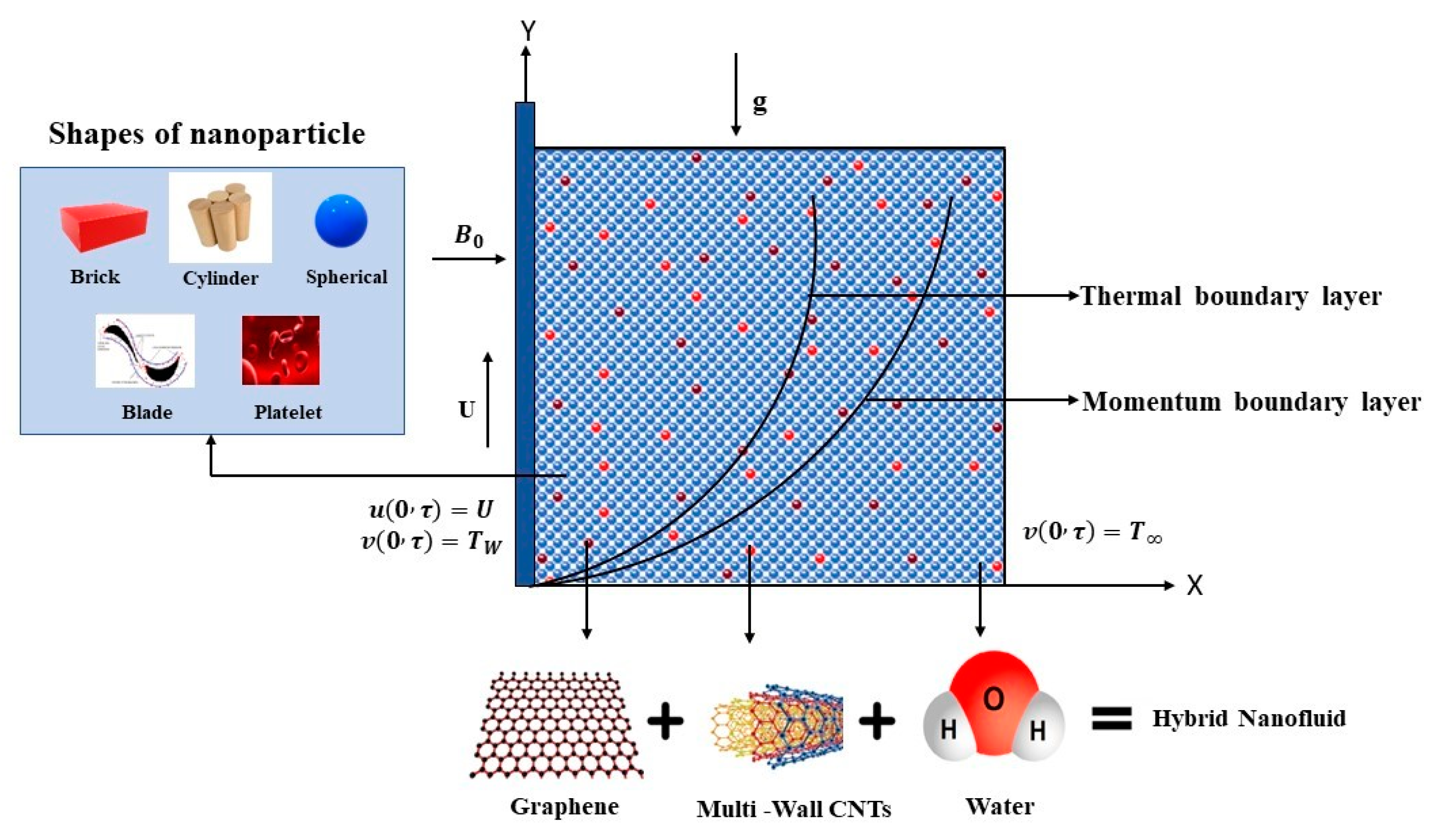
:1. Introduction
2. Fractional Mathematical Model with Caputo Derivative
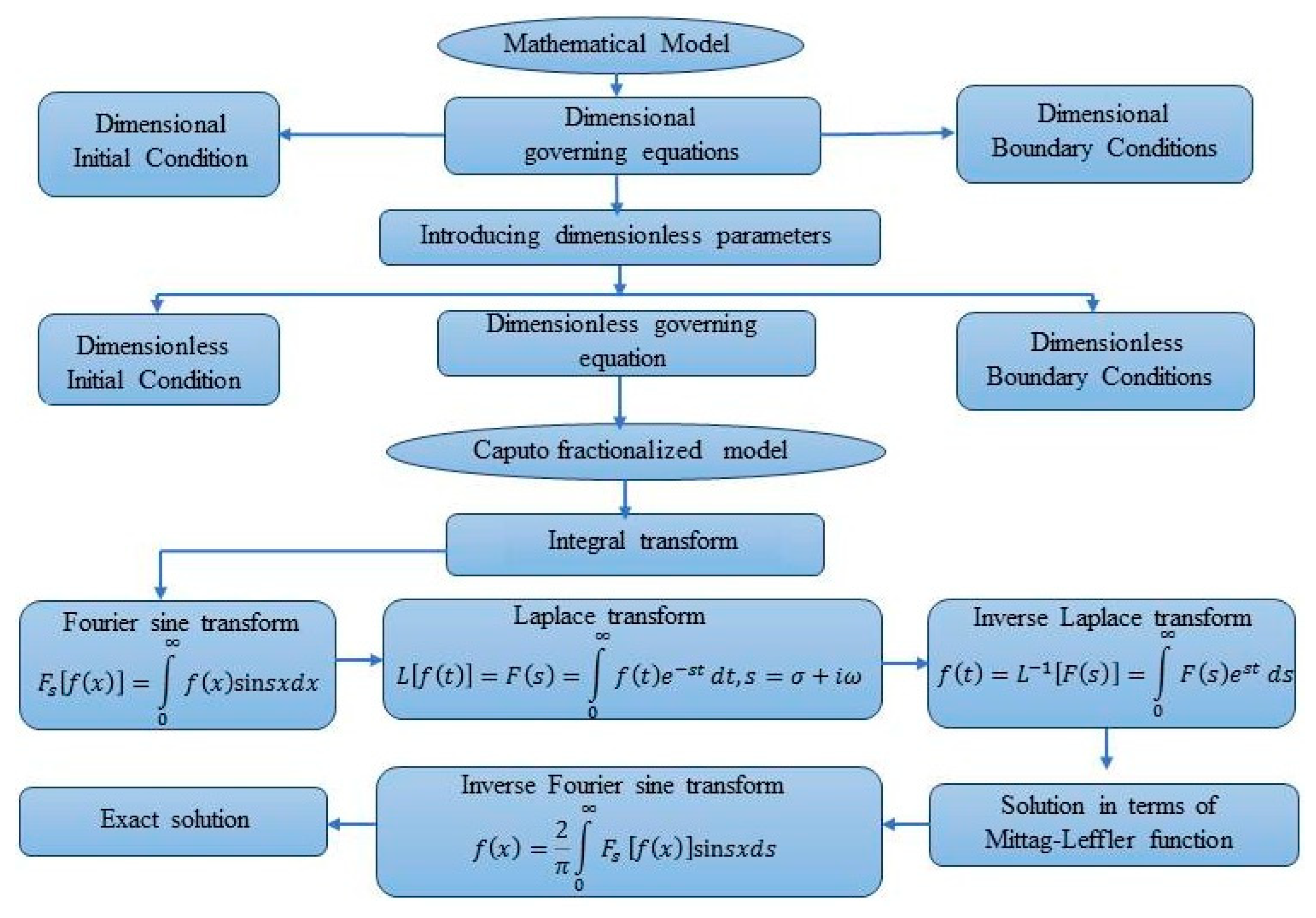
3. Procedure for Solution
3.1. Integral Transform for Fractional Order Caputo Derivative
3.2. Hybrid Fractional Temperature Field Calculation
3.3. Hybrid Fractional Velocity Field Calculation
3.4. Limiting Cases
3.4.1. Temperature Field for Classic Case with Hybrid Nanoparticles
3.4.2. Velocity Field for Classical Case with Hybrid Nanoparticles
3.4.3. Velocity Field for Classic Newtonian Fluid with Hybrid Nanoparticles
3.5. Analytical Expressions for the Heat Transfer and Shear Stress
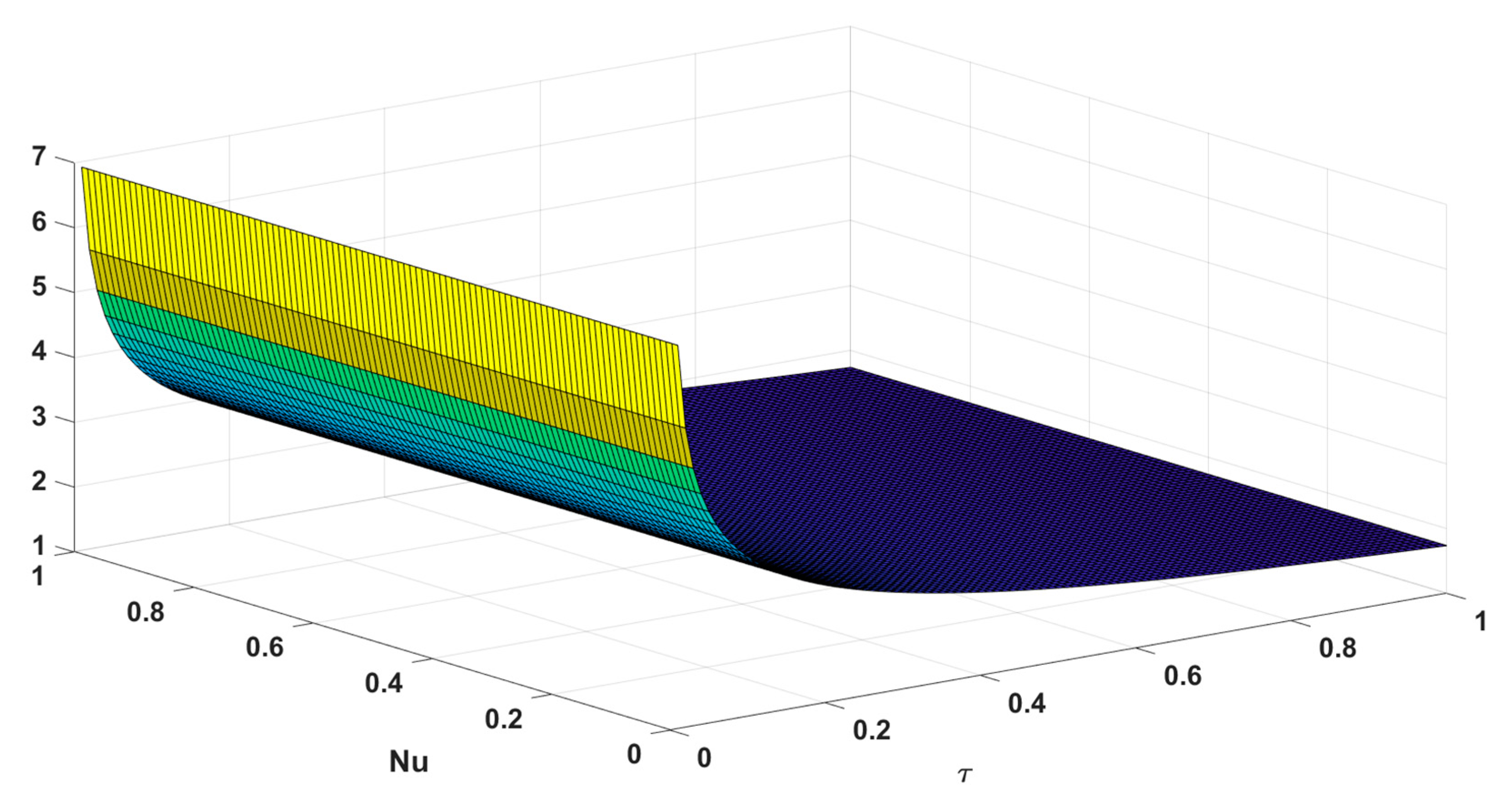
4. Graphical Findings and Outcomes
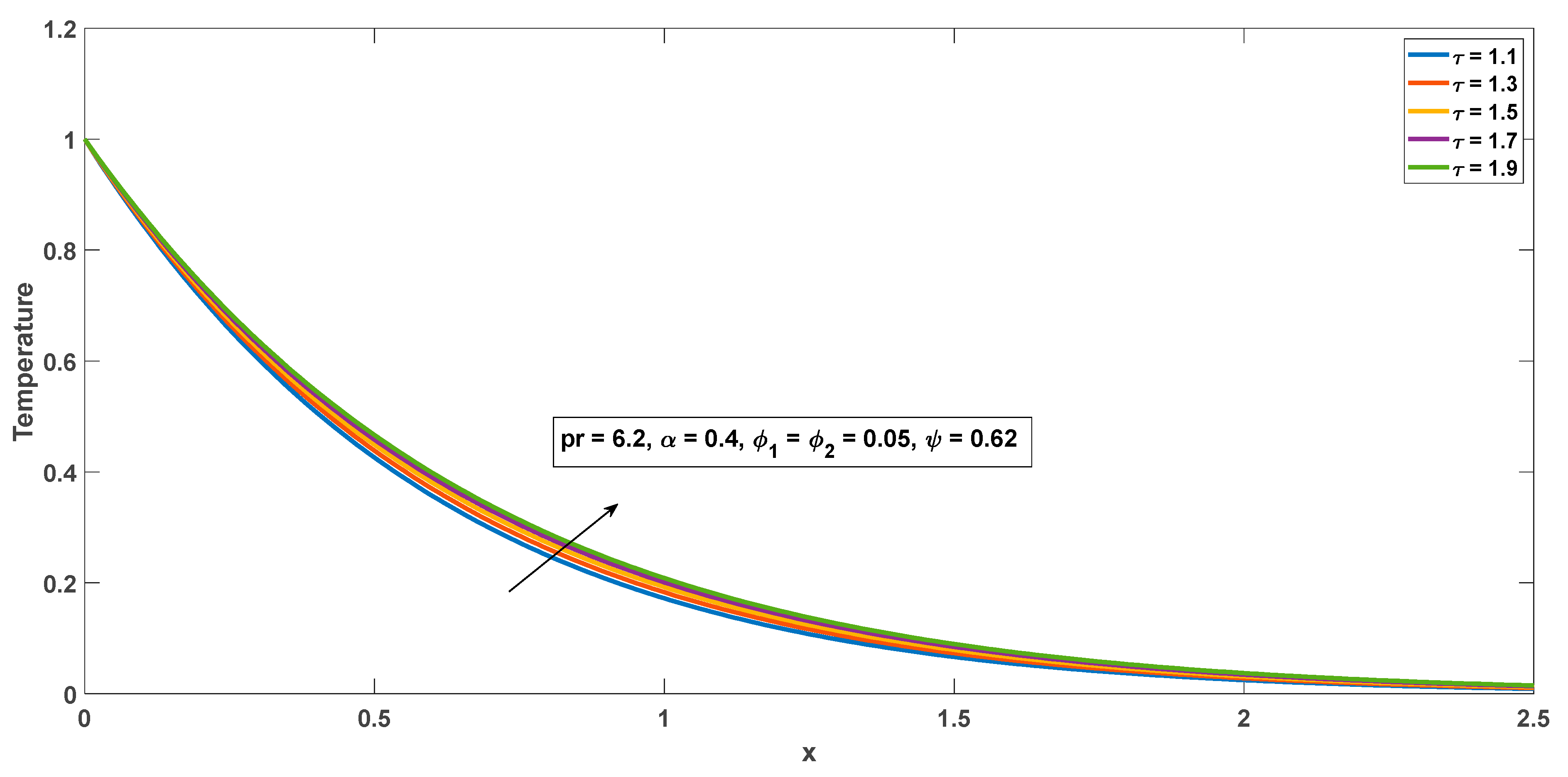
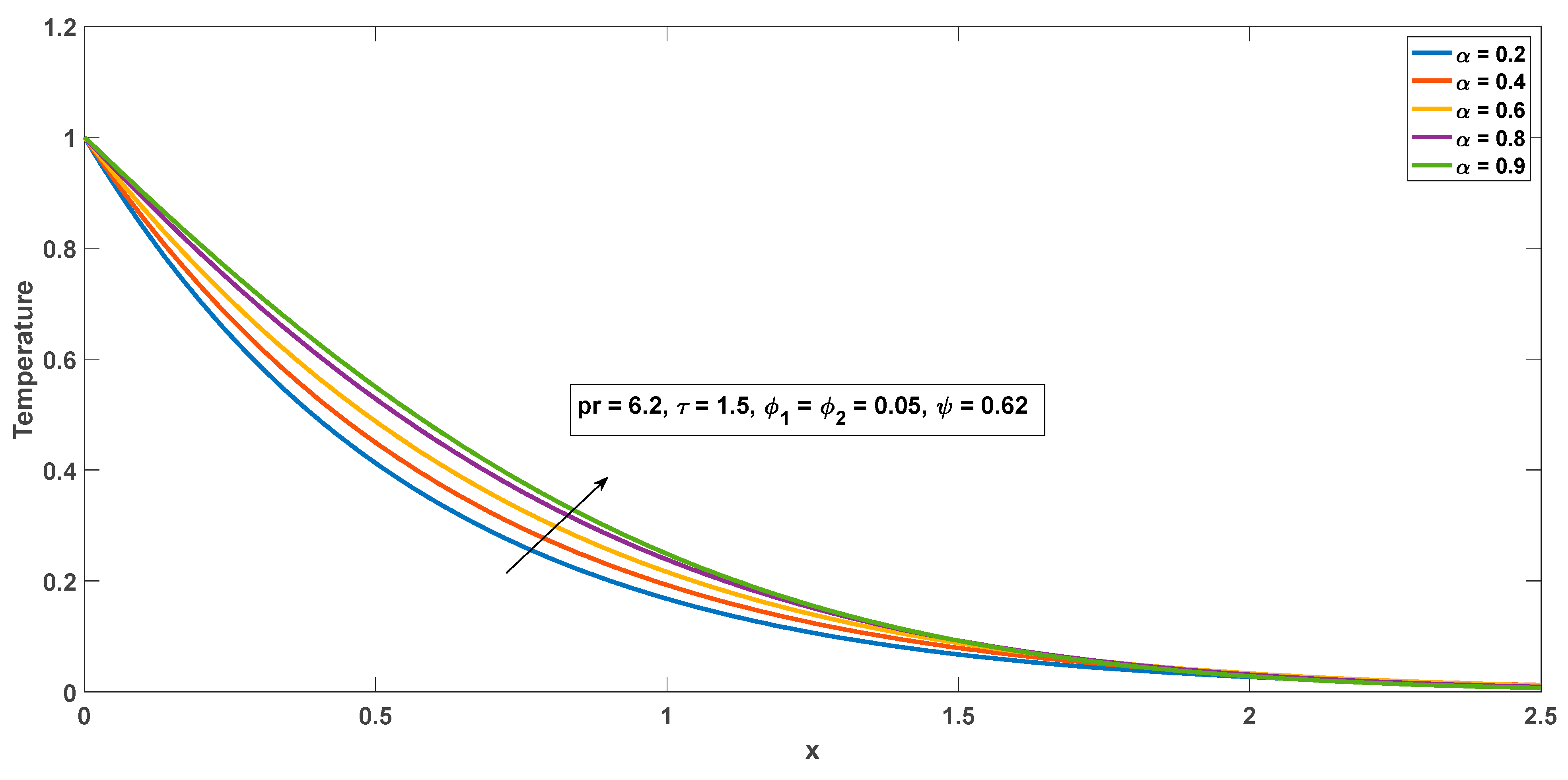
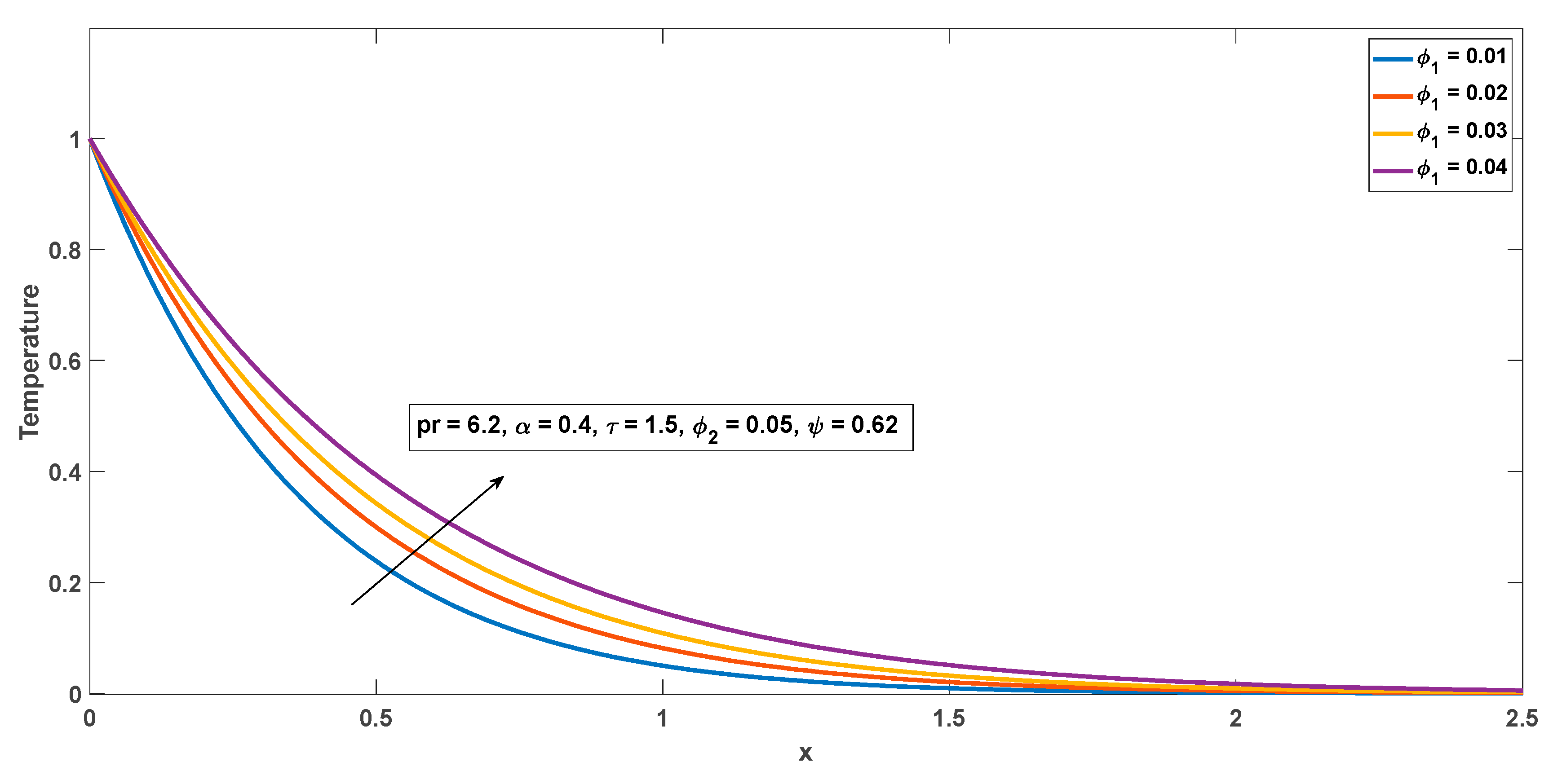
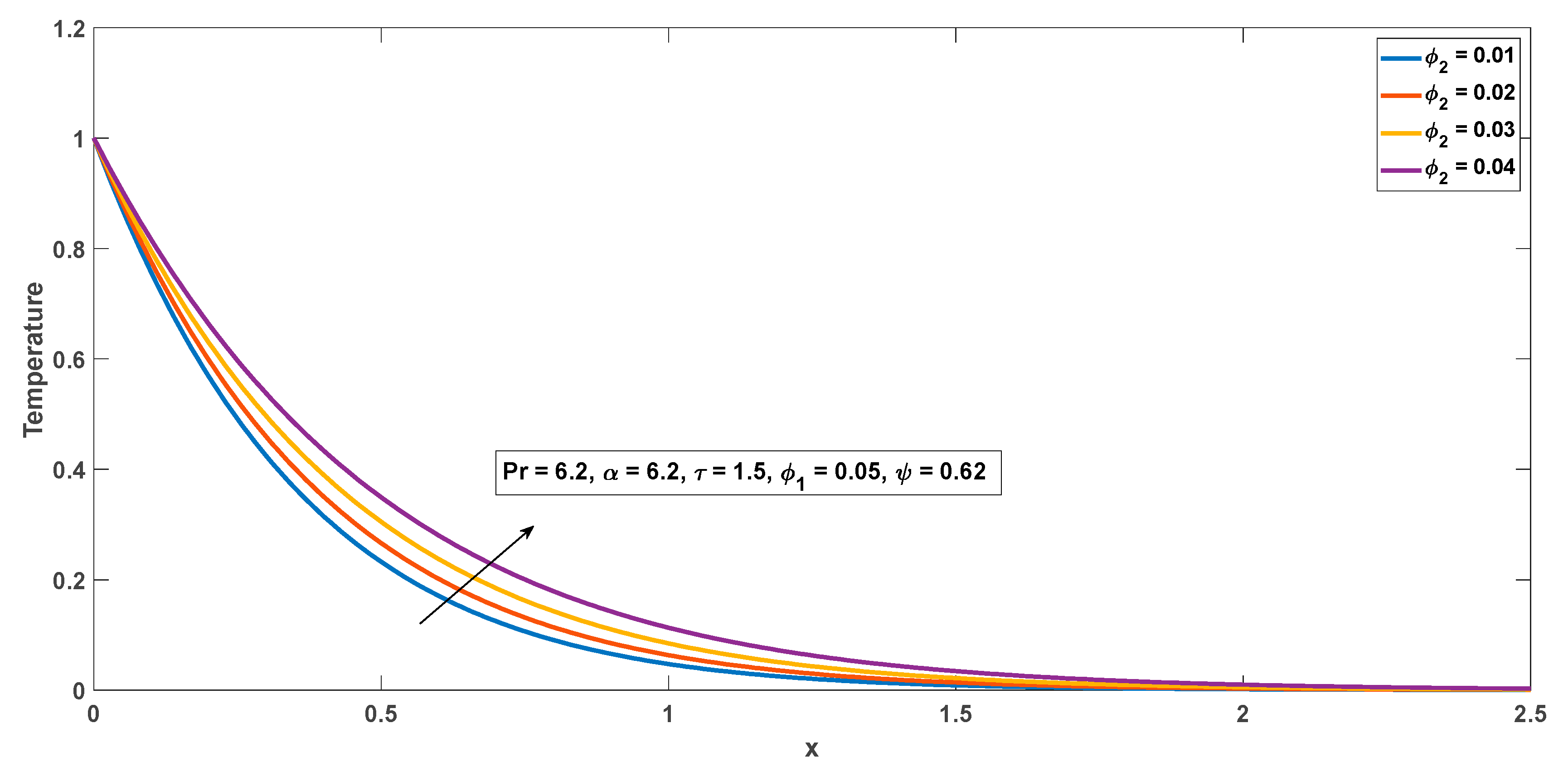
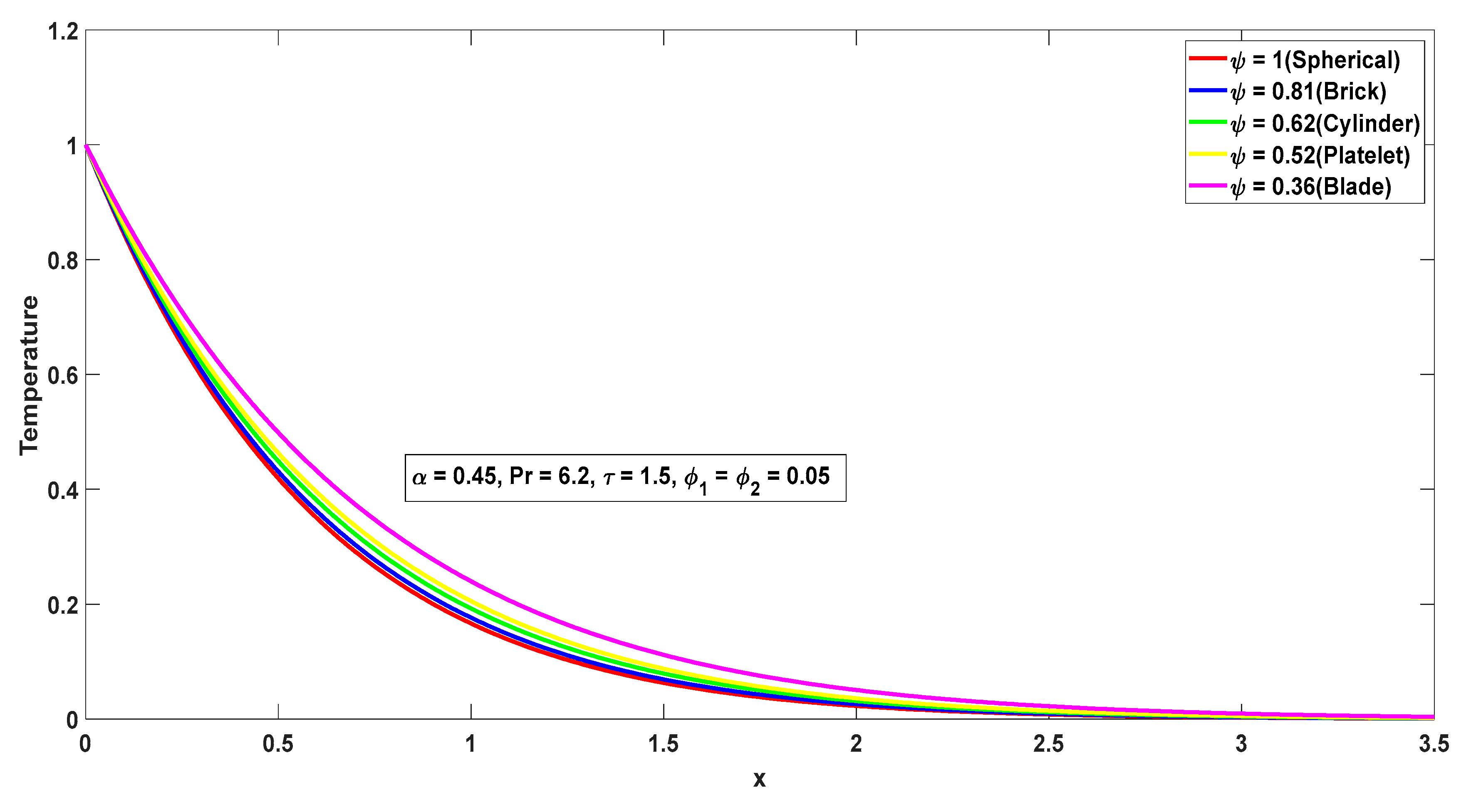
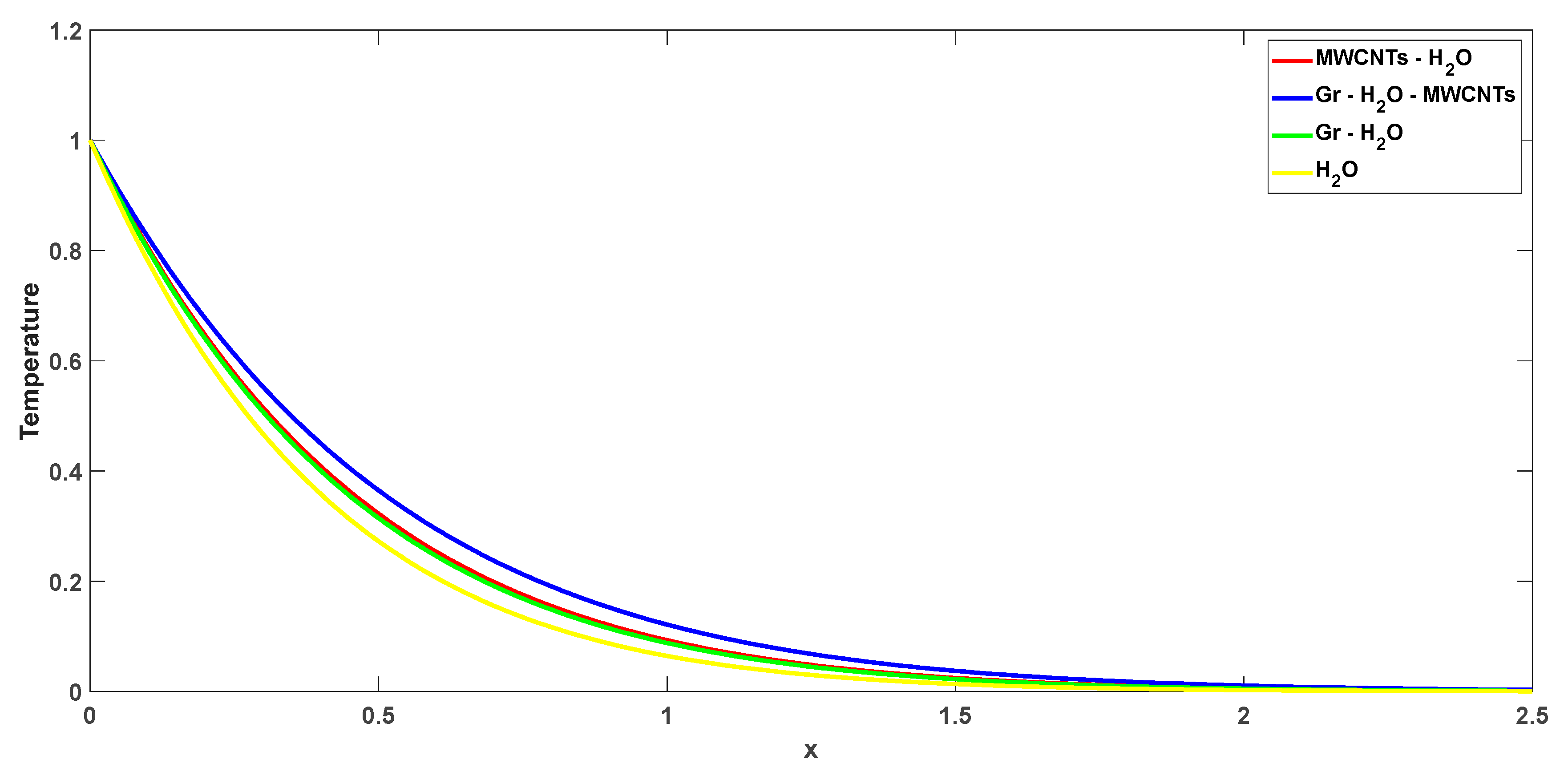
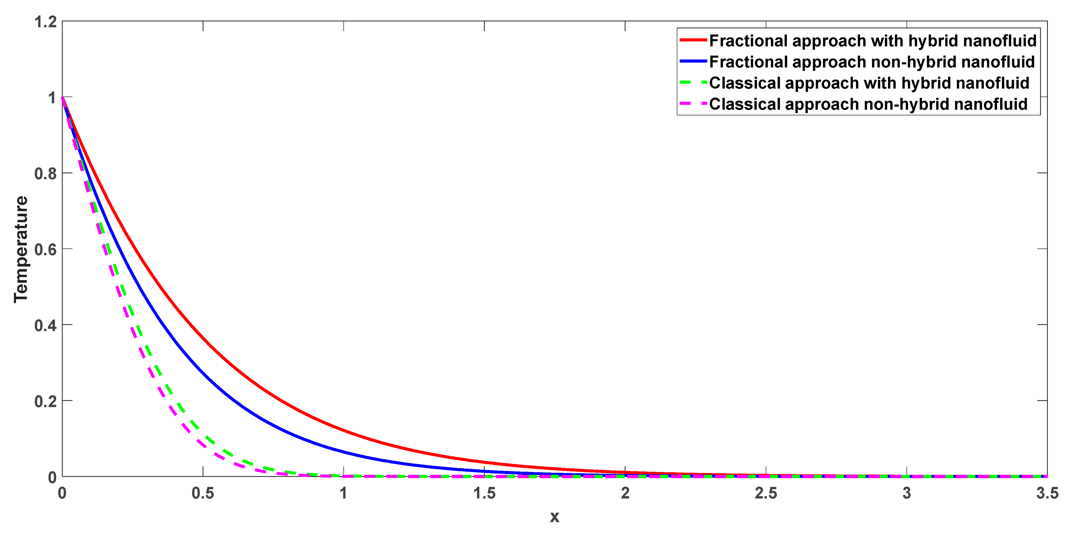
4.1. Impact of Physical Parameters on Temperature Field
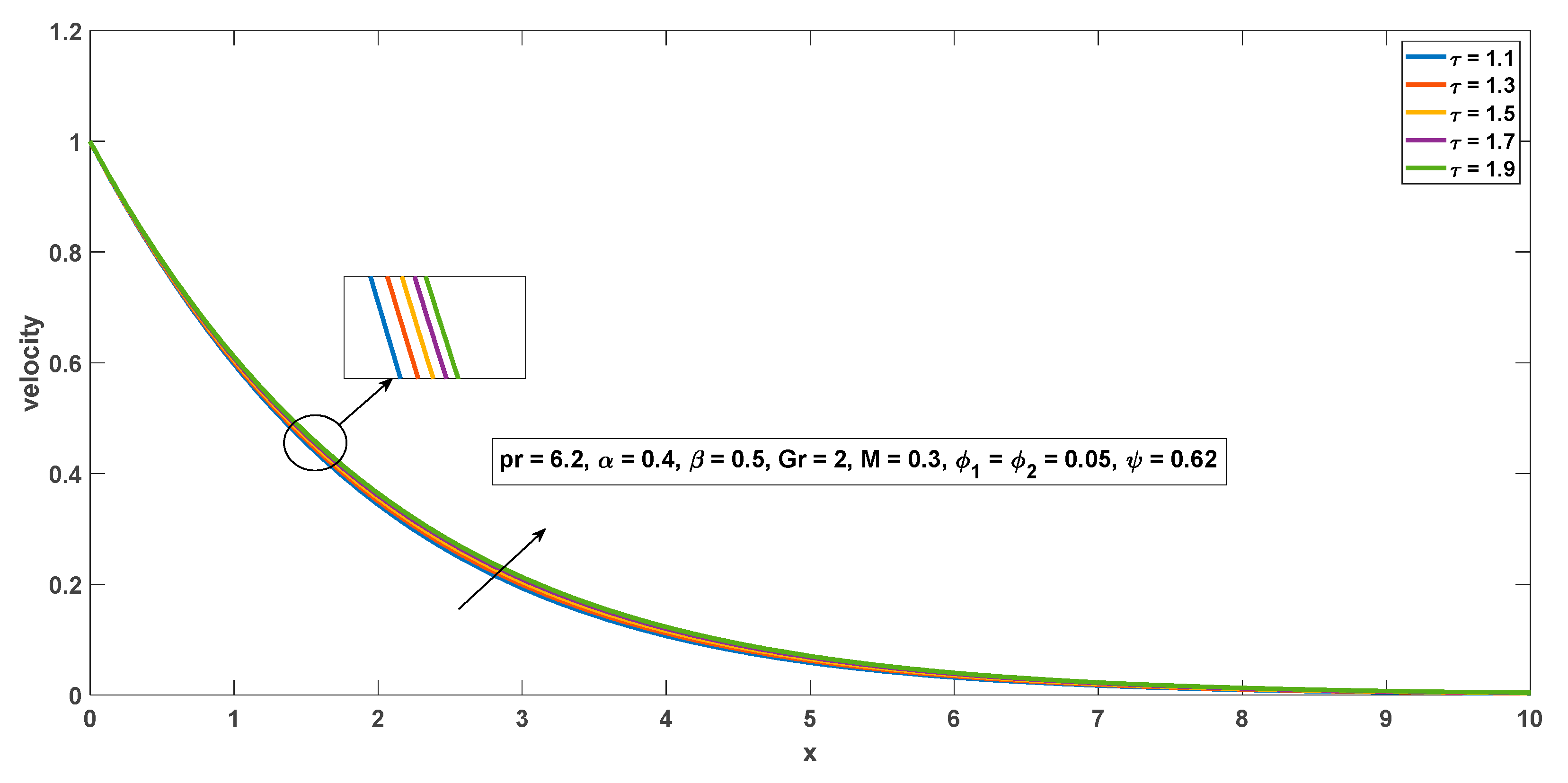
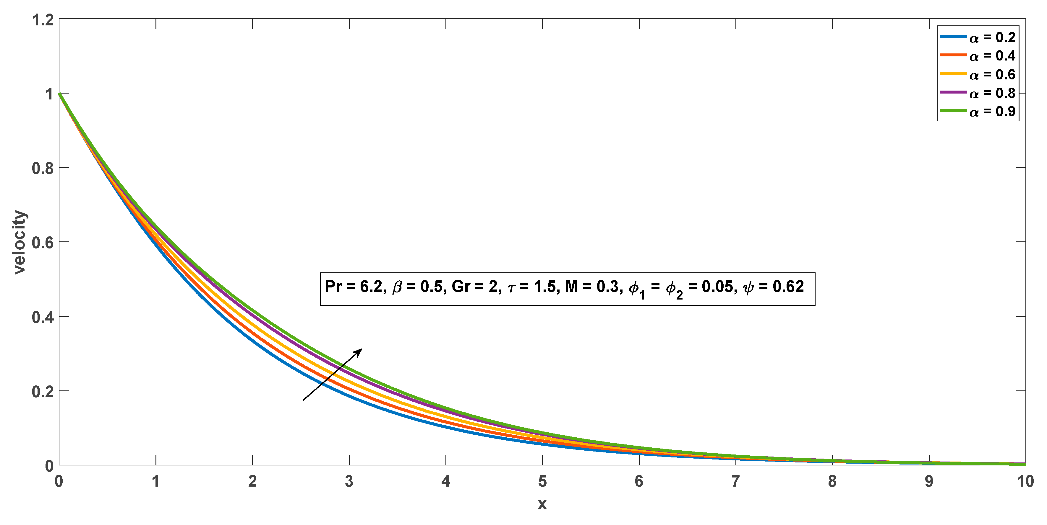
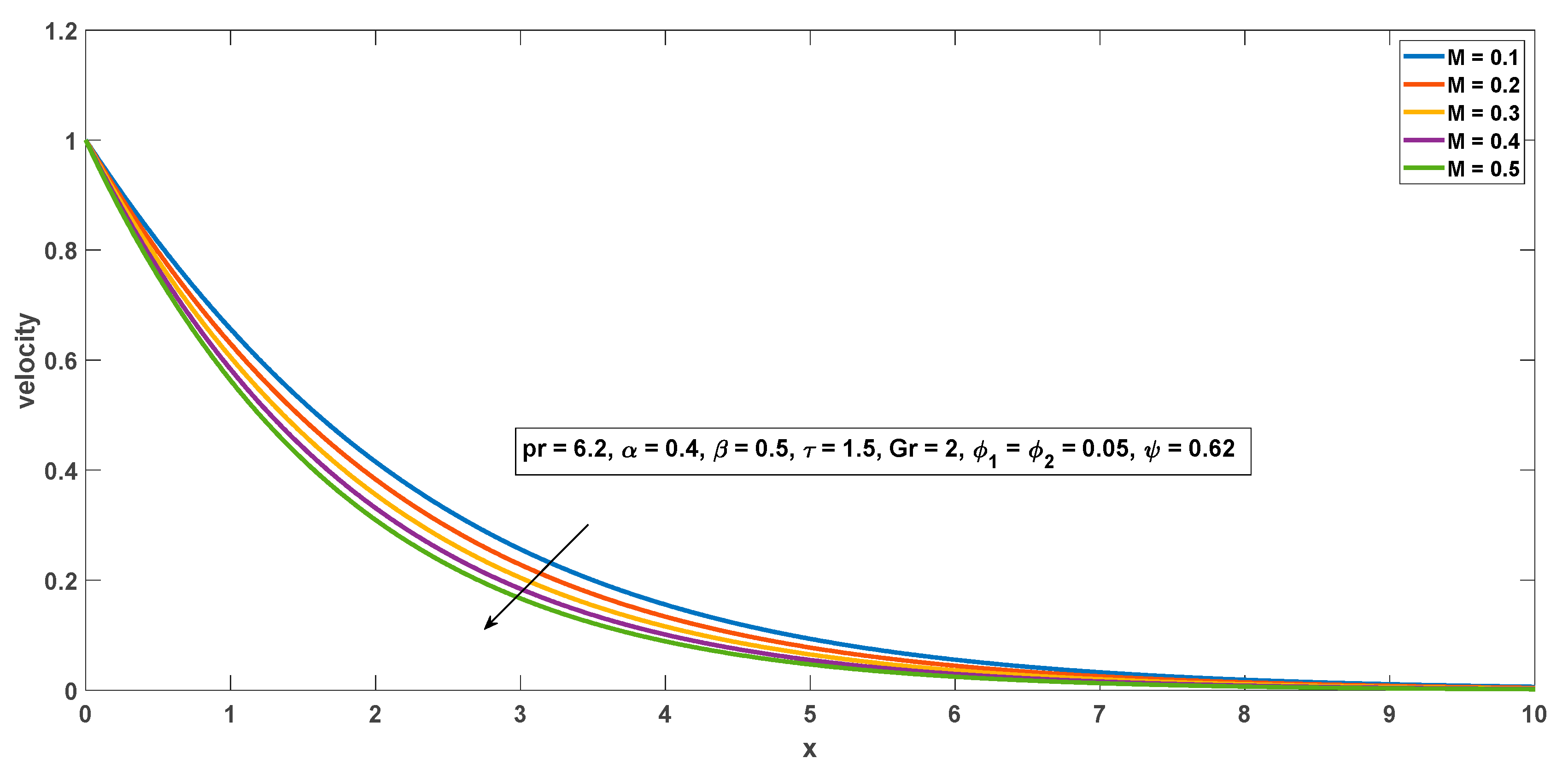
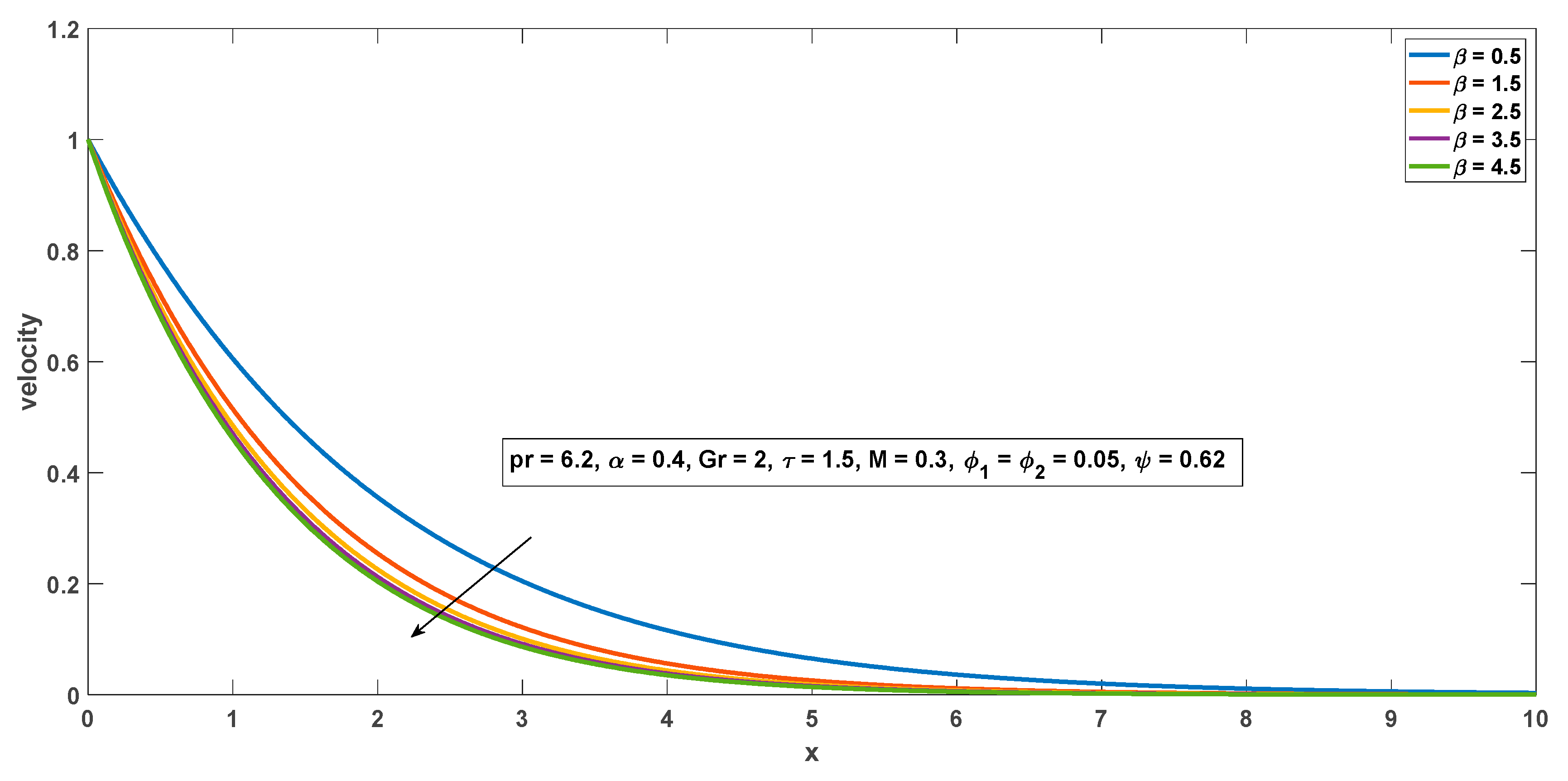
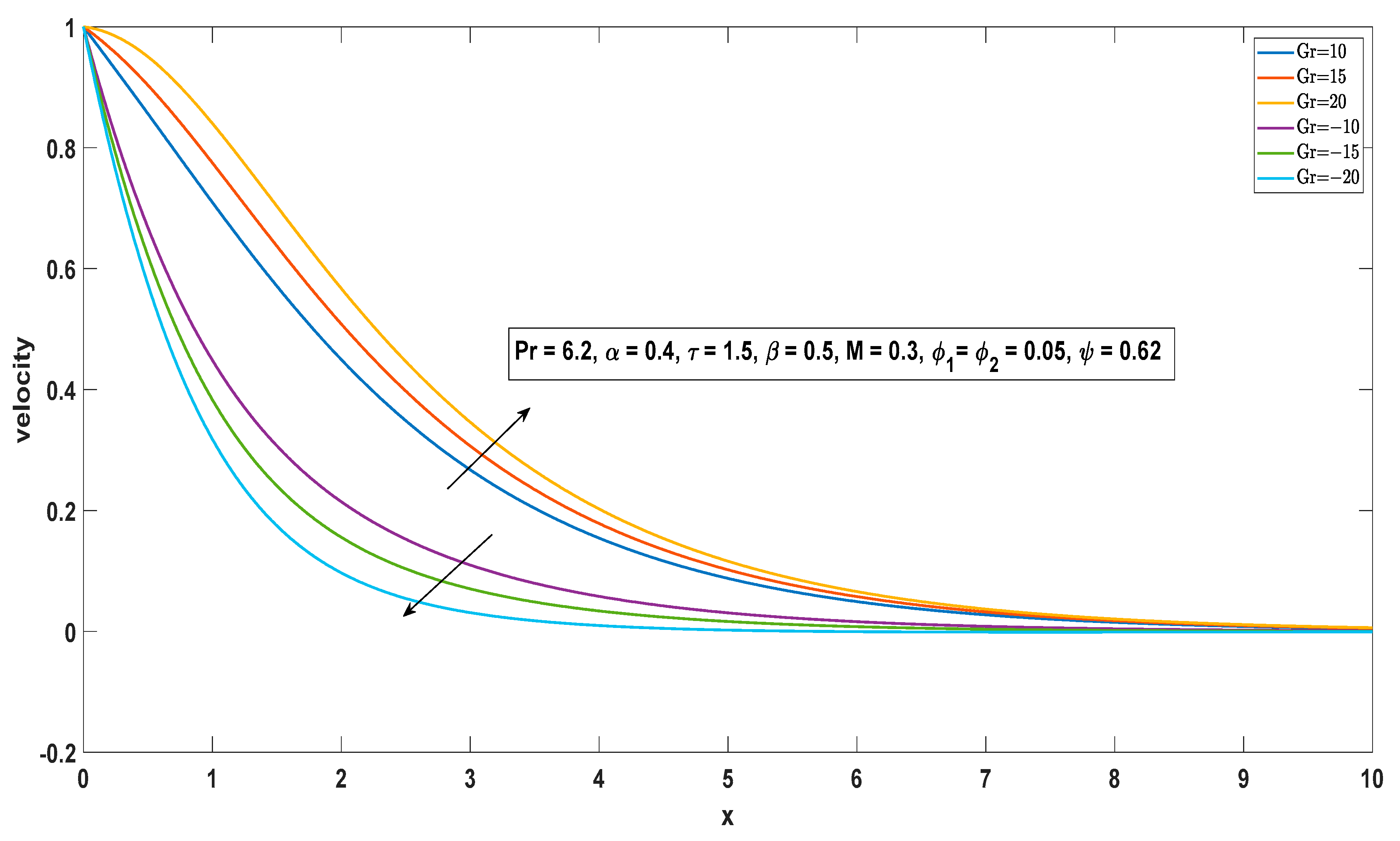
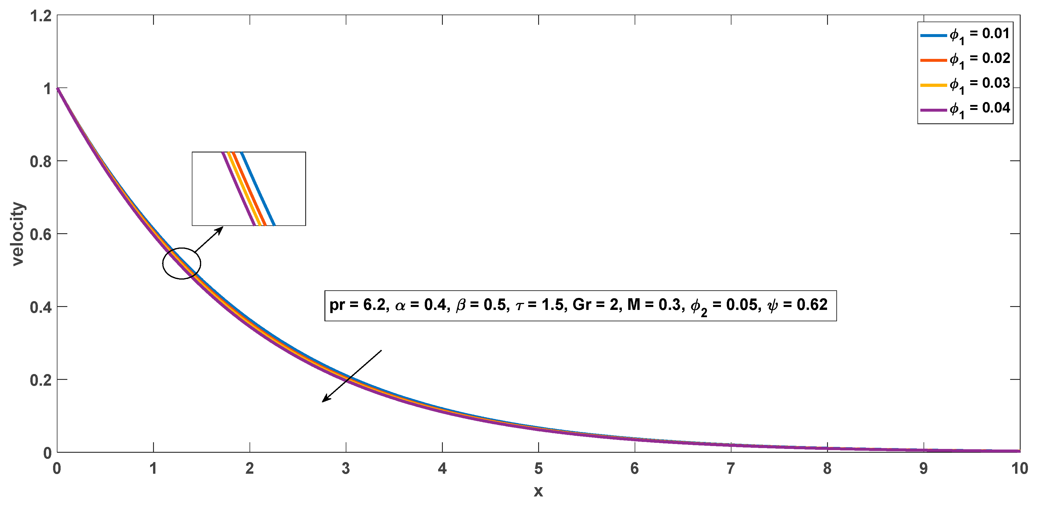
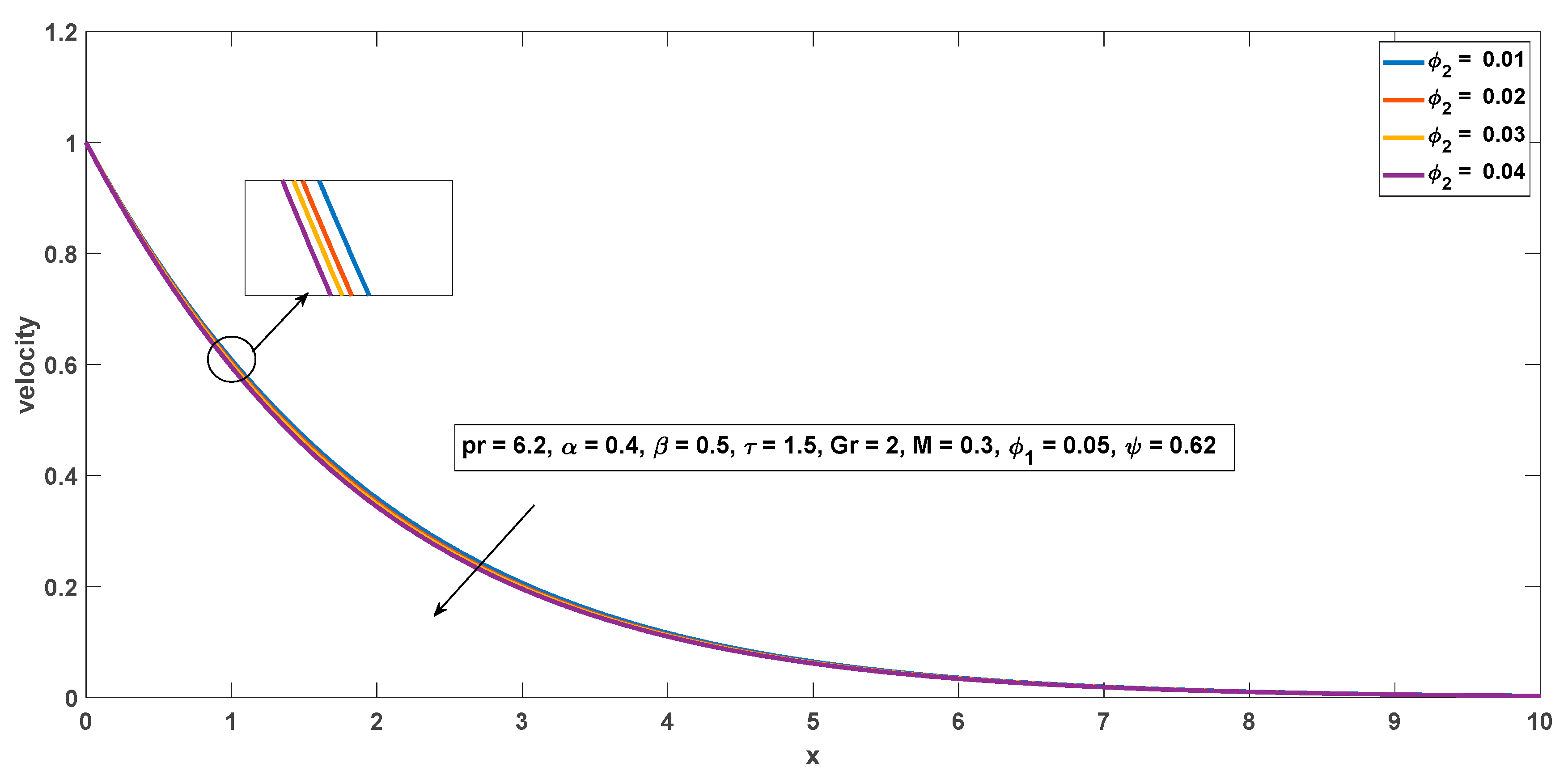
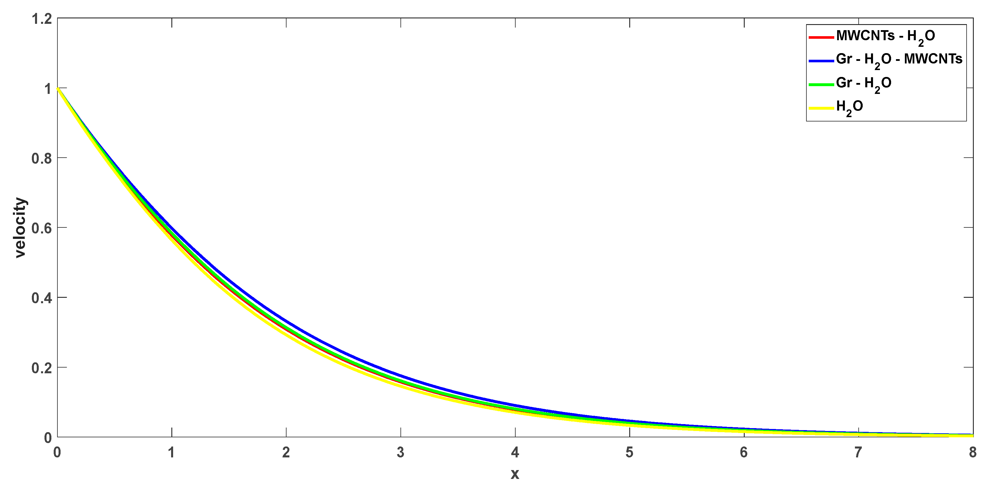
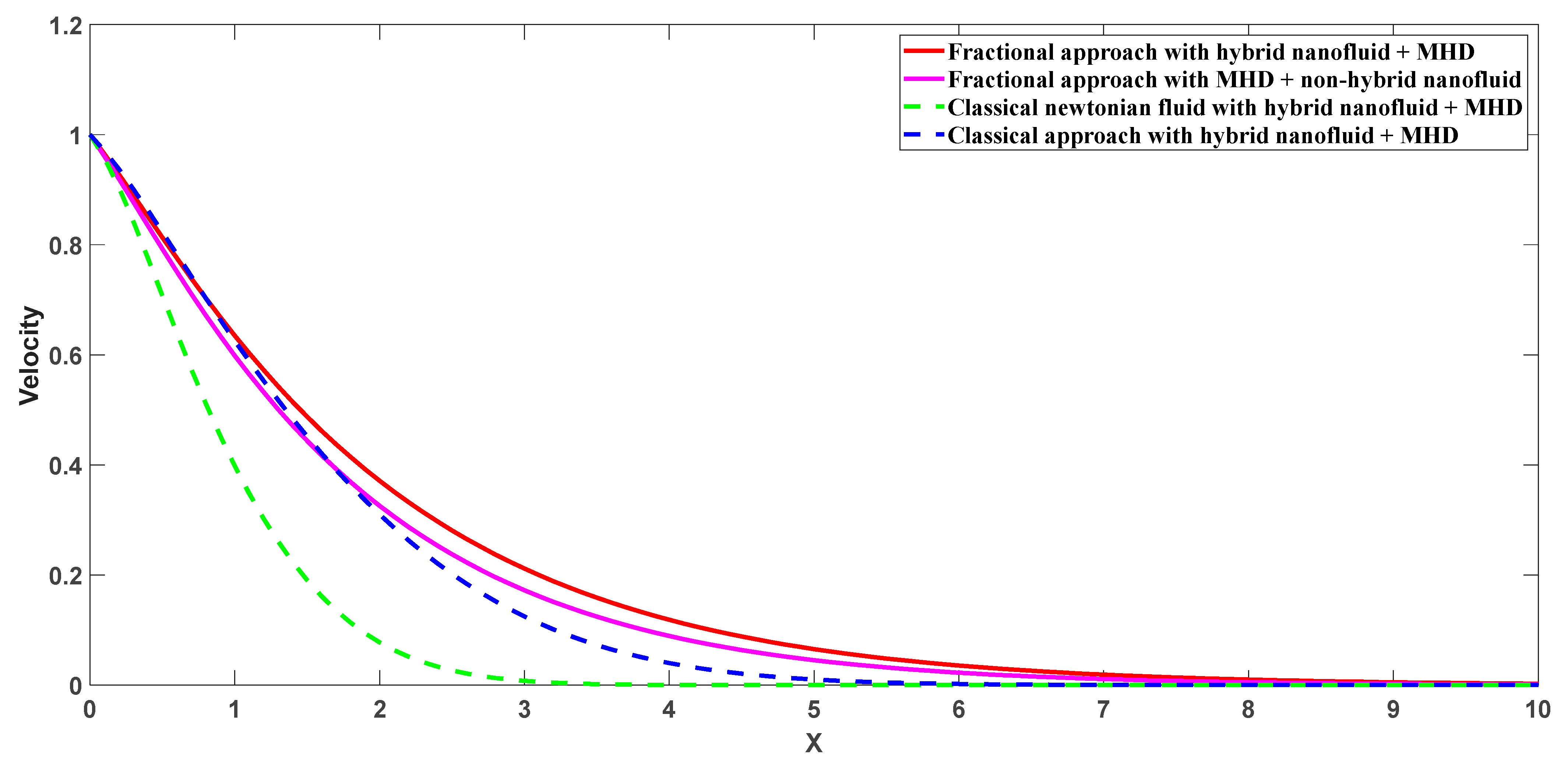
4.2. Impact of Physical Parameters on Flow Field
5. Conclusions
- The order of fractional derivatives can induce an increment or decrement in flow field and temperature depending on the time factor.
- In the case of cooling the plate, the fluid flow trend accelerates as the value of the Grashof number rises, whereas in the scenario of heating the plate, the reverse trend is observed.
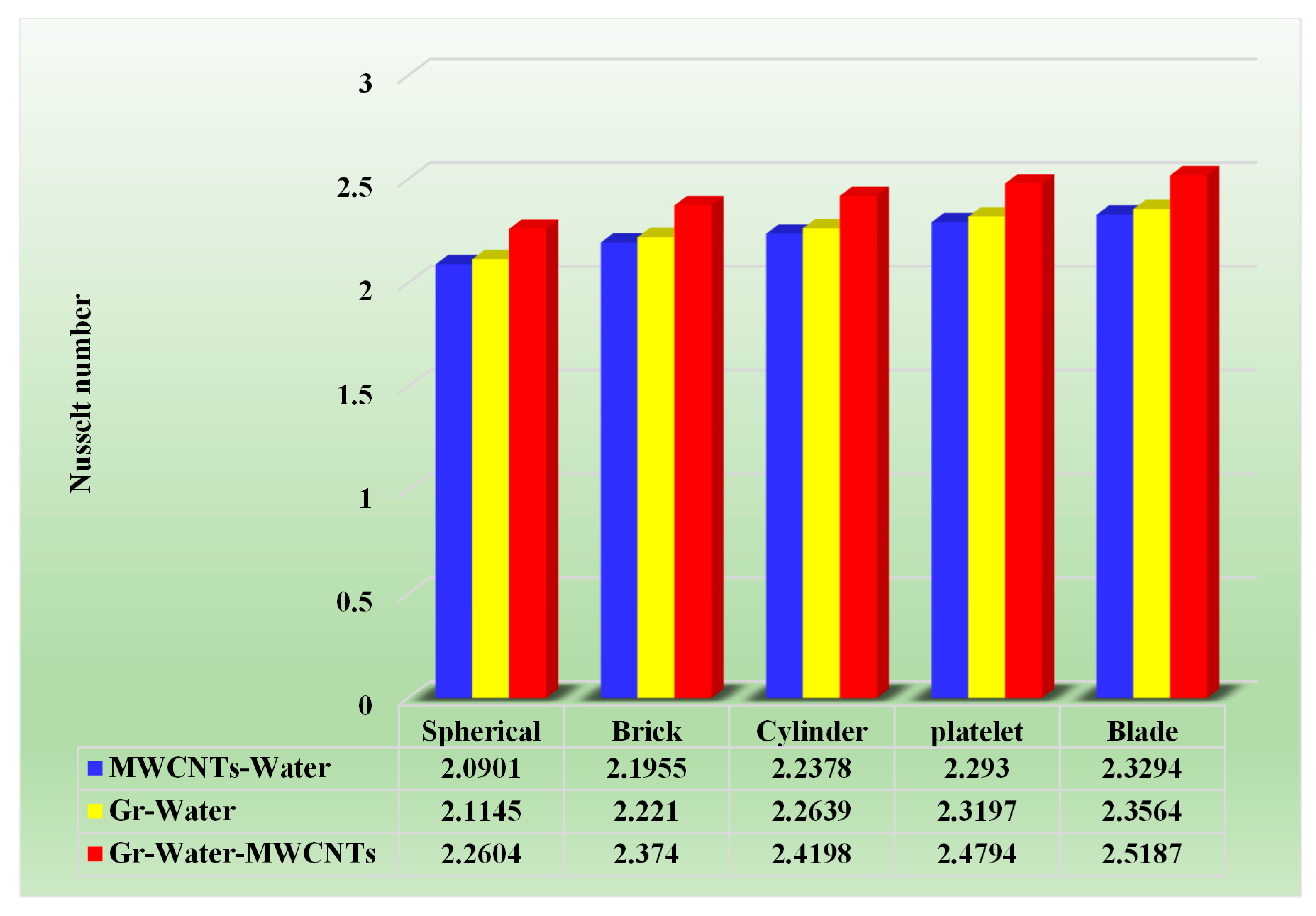
- Heat transmission rate of water-based hybrid nanofluid with cylindrical shaped nanoparticles are 4.9%, 9.5%, 13.7% and 17.7% greater as compared to regular fluid for volume fraction = 0.01 to 0.04, respectively.
- The blade-shaped hybrid nanoparticles are the most effective at increasing the heat transfer rate, whereas spherical nanoparticles perform at a lesser rate. These findings are significant in the long term because they help us plan for the improvement of heat transfer in cooling and heating applications.
- When compared to fluids with hybrid and non-hybrid nanofluids, fractional hybrid nanofluid shows the highest rate of heat transfer, whereas ordinary fluid shows minimum heat transmission rate. This demonstrates the fractional parameter improves fluid flow in a benchmark.
Author Contributions
Funding
Institutional Review Board Statement
Informed Consent Statement
Data Availability Statement
Conflicts of Interest
Nomenclature
| u | Velocity |
| v | Temperature |
| a, b | Shape constants |
| Pr | Prandtl number |
| Gr | Grashof number |
| Gr | Graphene nanoparticle |
| MWCNT | Multi wall carbon nanotube |
| MHD | Magnetohydrodynamics |
| x, y | Cartesian coordinates |
| Mittag-Leffler function | |
| Nu | Nusselt number |
| Cf | Skin friction coefficient |
| Greek symbols | |
| Density of nanofluid | |
| Specific heat capacity of nanofluid | |
| Thermal expansion coefficient of nanofluid | |
| Thermal conductivity of nanofluid | |
| Dynamic viscosity of nanofluid | |
| Electrical conductivity of nanofluid () | |
| Density of hybrid nanofluid | |
| Specific heat capacity of hybrid nanofluid | |
| Thermal expansion coefficient of hybrid nanofluid | |
| Thermal conductivity of hybrid nanofluid | |
| Dynamic viscosity of hybrid nanofluid | |
| Electrical conductivity of hybrid nanofluid () | |
| Specific gravity | |
| Magnetic field strength () | |
| Fractional parameter | |
| Casson parameter | |
| Time | |
| Volumetric coefficient of thermal expansion | |
| Sphericity of nanoparticles | |
| Volume fraction of Graphene | |
| Volume fraction of MWCNTs | |
| Subscripts | |
| f | Fluid |
| nf | Nanofluid |
| hnf | Hybrid nanofluid |
| np | Nanoparticle |
| w | Wall |
| Ambient condition |
References
- Maxwell, J.C. A Treatise on Electricity and Magnetism; Clarendon Press: London, UK, 1873. [Google Scholar]
- Choi, S.U.; Eastman, J.A. Enhancing Thermal Conductivity of Fluids with Nanoparticles; Argonne National Lab. (ANL): Argonne, IL, USA, 1995. [Google Scholar]
- Pîslaru-Dănescu, L.; Morega, A.M.; Telipan, G.; Morega, M.; Dumitru, J.B.; Marinescu, V. Magnetic nanofluid applications in electrical engineering. IEEE Trans. Magn. 2013, 49, 5489–5497. [Google Scholar] [CrossRef]
- Khodabandeh, E.; Safaei, M.R.; Akbari, S.; Akbari, O.A.; Alrashed, A.A. Application of nanofluid to improve the thermal performance of horizontal spiral coil utilized in solar ponds: Geometric study. Renew. Energy 2018, 122, 1–6. [Google Scholar] [CrossRef]
- Bahiraei, M.; Hangi, M. Investigating the efficacy of magnetic nanofluid as a coolant in double-pipe heat exchanger in the presence of magnetic field. Energy Convers. Manag. 2013, 76, 1125–1133. [Google Scholar] [CrossRef]
- Mekheimer, K.S.; Shahzadi, I.; Nadeem, S.; Moawad, A.M.; Zaher, A.Z. Reactivity of bifurcation angle and electroosmosis flow for hemodynamic flow through aortic bifurcation and stenotic wall with heat transfer. Phys. Scr. 2020, 96, 015216. [Google Scholar] [CrossRef]
- Ayub, M.; Shahzadi, I.; Nadeem, S. A ballon model analysis with Cu-blood medicated nanoparticles as drug agent through overlapped curved stenotic artery having compliant walls. Microsyst. Technol. 2019, 25, 2949–2962. [Google Scholar] [CrossRef]
- Siddique, I.; Sadiq, K.; Khan, I.; Nisar, K.S. Nanomaterials in convection flow of nanofluid in upright channel with gradients. J. Mater. Res. Technol. 2021, 11, 1411–1423. [Google Scholar] [CrossRef]
- Aleem, M.; Asjad, M.I.; Shaheen, A.; Khan, I. MHD Influence on different water based nanofluids (TiO2, Al2O3, CuO) in porous medium with chemical reaction and newtonian heating. Chaos Solit. Fractals 2020, 130, 109437. [Google Scholar] [CrossRef]
- Shafiq, A.; Hammouch, Z.; Sindhu, T.N. Bioconvective MHD flow of tangent hyperbolic nanofluid with newtonian heating. Int. J. Mech. Sci. 2017, 133, 759–766. [Google Scholar] [CrossRef]
- Yamada, A.; Sasabe, H.; Osada, Y.; Shiroda, Y.; Yamamoto, I. Concepts of Hybrid Materials, Hybrid Materials—Concept and Case Studies; ASM International: Novelty, OH, USA, 1989. [Google Scholar]
- Shahzadi, I.; Bilal, S.A. Significant role of permeability on blood flow for hybrid nanofluid through bifurcated stenosed artery: Drug delivery application. Comput. Methods Programs Biomed. 2020, 187, 105248. [Google Scholar] [CrossRef]
- Shahzadi, I.; Nadeem, S. Stimulation of metallic nanoparticles under the impact of radial magnetic field through eccentric cylinders: A useful application in biomedicine. J. Mol. Liq. 2017, 225, 365–381. [Google Scholar] [CrossRef]
- Shahzadi, I.; Nadeem, S. A comparative study of Cu nanoparticles under slip effects through oblique eccentric tubes, a biomedical solicitation examination. Can. J. Phys. 2019, 97, 63–81. [Google Scholar] [CrossRef]
- Javadi, H.; Urchueguia, J.F.; Mousavi Ajarostaghi, S.S.; Badenes, B. Impact of employing hybrid nanofluids as heat carrier fluid on the thermal performance of a borehole heat exchanger. Energies 2021, 14, 2892. [Google Scholar] [CrossRef]
- Jamshed, W.; Alanazi, A.K.; Isa, S.S.; Banerjee, R.; Eid, M.R.; Nisar, K.S.; Alshahrei, H.; Goodarzi, M. Thermal efficiency enhancement of solar aircraft by utilizing unsteady hybrid nanofluid: A single-phase optimized entropy analysis. Sustain. Energy Technol. Assess. 2022, 52, 101898. [Google Scholar] [CrossRef]
- Hafeez, M.U.; Hayat, T.; Alsaedi, A.; Khan, M.I. Numerical simulation for electrical conducting rotating flow of Au (Gold)-Zn (Zinc)/EG (Ethylene glycol) hybrid nanofluid. Int. Commun. Heat Mass Transf. 2021, 124, 105234. [Google Scholar] [CrossRef]
- Waini, I.; Ishak, A.; Groşan, T.; Pop, I. Mixed convection of a hybrid nanofluid flow along a vertical surface embedded in a porous medium. Int. Commun. Heat Mass Transf. 2020, 114, 104565. [Google Scholar] [CrossRef]
- Anwar, T.; Kumam, P.; Thounthong, P. A comparative fractional study to evaluate thermal performance of NaAlg–MoS2–Co hybrid nanofluid subject to shape factor and dual ramped conditions. Alex. Eng. J. 2022, 61, 2166–2187. [Google Scholar] [CrossRef]
- Balaji, T.; Rajendiran, S.; Selvam, C.; Lal, D.M. Enhanced heat transfer characteristics of water based hybrid nanofluids with graphene nanoplatelets and multi walled carbon nanotubes. Powder Technol. 2021, 394, 1141–1157. [Google Scholar] [CrossRef]
- Khan, M.; Lone, S.A.; Rasheed, A.; Alam, M.N. Computational simulation of Scott-Blair model to fractional hybrid nanofluid with Darcy medium. Int. Commun. Heat Mass Transf. 2022, 130, 105784. [Google Scholar] [CrossRef]
- Roy, N.C.; Pop, I. Analytical investigation of transient free convection and heat transfer of a hybrid nanofluid between two vertical parallel plates. Phys. Fluids 2022, 34, 072005. [Google Scholar] [CrossRef]
- Sene, N. Analytical investigations of the fractional free convection flow of Brinkman type fluid described by the Caputo fractional derivative. Results Phys. 2022, 37, 105555. [Google Scholar] [CrossRef]
- Khan, Z.A.; Haq, S.U.; Khan, T.S.; Khan, I.; Nisar, K.S. Fractional Brinkman type fluid in channel under the effect of MHD with Caputo-Fabrizio fractional derivative. Alex. Eng. J. 2020, 59, 2901–2910. [Google Scholar] [CrossRef]
- Reyaz, R.; Lim, Y.J.; Mohamad, A.Q.; Saqib, M.; Shafie, S. Caputo fractional MHD Casson Fluid flow over an oscillating plate with thermal radiation. J. Adv. Res. Fluid Mech. Therm. Sci. 2021, 85, 145–158. [Google Scholar] [CrossRef]
- Casson, N. A flow equation for pigment-oil suspensions of the printing ink type. Rheol. Disperse Syst. 1959, 10021830093. [Google Scholar]
- Raza, A.; Khan, S.U.; Farid, S.; Khan, M.I.; Sun, T.C.; Abbasi, A.; Khan, M.I.; Malik, M.Y. Thermal activity of conventional Casson nanoparticles with ramped temperature due to an infinite vertical plate via fractional derivative approach. Case Stud. Therm. Eng. 2021, 27, 101191. [Google Scholar] [CrossRef]
- Shahrim, M.N.; Mohamad, A.Q.; Jiann, L.Y.; Zakaria, M.N.; Shafie, S.; Ismail, Z.; Kasim, A.R. Exact solution of fractional convective Casson Fluid through an accelerated plate. CFD Lett. 2021, 13, 15–25. [Google Scholar] [CrossRef]
- Krishna, M.V.; Ahammad, N.A.; Chamkha, A.J. Radiative MHD flow of Casson hybrid nanofluid over an infinite exponentially accelerated vertical porous surface. Case Stud. Therm. Eng. 2021, 27, 101229. [Google Scholar] [CrossRef]
- Kilbas, A.A.; Srivastava, H.M.; Trujillo, J.J. Theory and Applications of Fractional Differential Equations; North-Holland Mathematics Studies; Elsevier: Amsterdam, The Netherlands, 2006. [Google Scholar]
- Caputo, M. Linear models of dissipation whose Q is almost frequency independent—II. Geophys. J. Int. 1967, 13, 529–539. [Google Scholar] [CrossRef]
- Anwar, T.; Kumam, P. A fractal fractional model for thermal analysis of GO− NaAlg− Gr hybrid nanofluid flow in a channel considering shape effects. Case Stud. Therm. Eng. 2022, 31, 101828. [Google Scholar] [CrossRef]
- Saqib, M.; Khan, I.; Shafie, S. Application of Atangana–Baleanu fractional derivative to MHD channel flow of CMC-based-CNT’s nanofluid through a porous medium. Chaos Solit. Fractals 2018, 116, 79–85. [Google Scholar] [CrossRef]
- Daud, M.M.; Jiann, L.Y.; Mahat, R.; Shafie, S. Application of Caputo Fractional Derivatives to the Convective Flow of Casson Fluids in a Microchannel with Thermal Radiation. J. Adv. Res. Fluid Mech. Therm. Sci. 2022, 93, 50–63. [Google Scholar] [CrossRef]
- Ahmad, M.; Imran, M.A.; Nazar, M. Mathematical modeling of (Cu− A l 2 O 3) water based Maxwell hybrid nanofluids with Caputo-Fabrizio fractional derivative. Adv. Mech. Eng. 2020, 12, 1687814020958841. [Google Scholar] [CrossRef]
- Aman, S.; Zokri, S.M.; Ismail, Z.; Salleh, M.Z.; Khan, I. Casson model of MHD flow of SA-based hybrid nanofluid using Caputo time-fractional models. Defect Diffus. 2019, 390, 83–90. [Google Scholar] [CrossRef]
- Sene, N. Analytical solutions of a class of fluids models with the Caputo fractional derivative. Fractal Fract. 2022, 6, 35. [Google Scholar] [CrossRef]
- Nakamura, M.; Sawada, T. Numerical study on the flow of a non-Newtonian fluid through an axisymmetric stenosis. J. Biomech. Eng. 1990, 112, 100–103. [Google Scholar] [CrossRef] [PubMed]
- Shah, N.A.; Khan, I. Heat transfer analysis in a second grade fluid over and oscillating vertical plate using fractional Caputo–Fabrizio derivatives. Eur. Phys. J. C 2016, 76, 362. [Google Scholar] [CrossRef]
- Reddy, S.R.; Reddy, P.B. Entropy generation analysis on MHD flow with a binary mixture of ethylene glycol and water based silver-graphene hybrid nanoparticles in automotive cooling systems. Int. J. Heat Technol. 2021, 39, 1781–1790. [Google Scholar] [CrossRef]
- Curtis, W.D.; Logan, J.D.; Parker, W.A. Dimensional analysis and the pi theorem. Linear Algebra Its Appl. 1982, 47, 117–126. [Google Scholar] [CrossRef]
- Sene, N. Stokes’ first problem for heated flat plate with Atangana–Baleanu fractional derivative. Chaos Solit. Fractals 2018, 117, 68–75. [Google Scholar] [CrossRef]
- Abro, K.A.; Khan, I.; Gómez-Aguilar, J.F. Thermal effects of magnetohydrodynamic micropolar fluid embedded in porous medium with Fourier Sine Transform technique. J. Braz. Soc. Mech. Sci. Eng. 2019, 41, 174. [Google Scholar] [CrossRef]
- Podlubny, I. Fractional Differential Equations, Mathematics in Science and Engineering; Academic Press: New York, NY, USA, 1999. [Google Scholar]
- Soundalgekar, V.M. Free convection effect on the stokes problem for a vertical plate in an elasto-viscous fluid. Czechoslov. J. Phys. 1978, 28, 721–727. [Google Scholar] [CrossRef]


| Properties | Hybrid Nanofluid |
|---|---|
| Viscosity, | (Brinkman model) |
| Density, | |
| Specific heat capacity, | |
| Thermal conductivity, | (Maxwell model) where |
| Electrical conductivity, | where |
| Thermal expansion coefficient, |
| Physical Properties | Water (H2O) | Graphene (Gr) | Multiwall Carbon Nanotube (MWCNT) |
|---|---|---|---|
| / | 997.1 | 2250 | 1600 |
| / | 4179 | 2100 | 796 |
| / | 0.613 | 2500 | 3000 |
| Models | a | b | ||
|---|---|---|---|---|
| Blade | 14.6 | 123.3 | 0.36 | 8.3 |
| Brick | 1.9 | 471.4 | 0.81 | 3.7 |
| Platelet | 37.1 | 612.6 | 0.52 | 5.7 |
| Cylinder | 13.5 | 909.4 | 0.62 | 4.9 |
| Spherical | - | - | 1 | 3 |
| Pr | |||||
|---|---|---|---|---|---|
| 0.02 | 0.02 | 6.2 | 0.6 | 1.5 | 1.591572294587753 |
| 0.03 | - | - | - | - | 1.569480227825062 |
| 0.04 | - | - | - | - | 1.547886513587993 |
| - | 0.03 | - | - | - | 1.562898376223181 |
| - | 0.04 | - | - | - | 1.534893820304120 |
| - | - | 8 | - | - | 1.807904639541740 |
| - | - | 9 | - | - | 1.917572445537878 |
| - | - | - | 0.8 | - | 1.332170104172774 |
| - | - | - | 0.9 | - | 1.202904460764115 |
| - | - | - | - | 1.7 | 1.532918522253240 |
| - | - | - | - | 1.8 | 1.506856850036236 |
| Pr | % Increased | |||||
|---|---|---|---|---|---|---|
| 0.00 | 0.00 | 6.2 | 0.4 | 1.5 | 1.9721 | - |
| 0.01 | 0.01 | 6.2 | 0.4 | 1.5 | 1.8751 | 4.9 |
| 0.02 | 0.02 | 6.2 | 0.4 | 1.5 | 1.7850 | 9.5 |
| 0.03 | 0.03 | 6.2 | 0.4 | 1.5 | 1.7011 | 13.7 |
| 0.04 | 0.04 | 6.2 | 0.4 | 1.5 | 1.6229 | 17.7 |
| 0.01 | 0.01 | 1.9506 | 1.9545 | 1.9562 | 1.9594 | 1.9421 | 1.9341 | 1.9301 | 1.9139 |
| 0.02 | 0.02 | 1.9291 | 1.9368 | 1.9402 | 1.9467 | 1.9122 | 1.8965 | 1.8888 | 1.8577 |
| 0.03 | 0.03 | 1.9076 | 1.9190 | 1.9241 | 1.9338 | 1.8826 | 1.8596 | 1.8482 | 1.8034 |
| 0.04 | 0.04 | 1.8860 | 1.9012 | 1.9079 | 1.9208 | 1.8532 | 1.8231 | 1.8085 | 1.7509 |
| Pr | Gr | M | ||||||
|---|---|---|---|---|---|---|---|---|
| 0.03 | 0.03 | 6.2 | 0.45 | 0.5 | 1.5 | 2 | 2 | 0.959525615427890 |
| 0.04 | - | - | - | - | - | - | - | 0.952001945188767 |
| 0.05 | - | - | - | - | - | - | - | 0.944169083022009 |
| - | 0.04 | - | - | - | - | - | - | 0.966946221691135 |
| - | 0.05 | - | - | - | - | - | - | 0.974469891930258 |
| - | - | 12 | - | - | - | - | - | 0.942932315311468 |
| - | - | 15 | - | - | - | - | - | 0.944117551034069 |
| - | - | - | 0.65 | - | - | - | - | 1.094127167925078 |
| - | - | - | 0.9 | - | - | - | - | 1.246661852225108 |
| - | - | - | - | 0.7 | - | - | - | 1.091373887426613 |
| - | - | - | - | 0.9 | - | - | - | 1.206821899771669 |
| - | - | - | - | - | 2.5 | - | - | 1.061352823595748 |
| - | - | - | - | - | 4.5 | - | - | 1.151739930441103 |
| - | - | - | - | - | - | 4 | - | 0.877486690628685 |
| - | - | - | - | - | - | 6 | - | 0.796478405588264 |
| - | - | - | - | - | - | - | 3 | 1.131848583096572 |
| - | - | - | - | - | - | - | 5 | 1.422179803146021 |
| Pr | Classic Approach (Soundalgekar V.M [45]) | Fractional Approach | Difference |
|---|---|---|---|
| 0.71 | 0.3994 | 0.4029 | 0.0035 |
| 1.0 | 0.0082 | 0.0117 | 0.0035 |
| 1.5 | 0.3173 | 0.3234 | 0.0061 |
| 7.0 | 0.2207 | 0.2295 | 0.0088 |
Disclaimer/Publisher’s Note: The statements, opinions and data contained in all publications are solely those of the individual author(s) and contributor(s) and not of MDPI and/or the editor(s). MDPI and/or the editor(s) disclaim responsibility for any injury to people or property resulting from any ideas, methods, instructions or products referred to in the content. |
© 2023 by the authors. Licensee MDPI, Basel, Switzerland. This article is an open access article distributed under the terms and conditions of the Creative Commons Attribution (CC BY) license (https://creativecommons.org/licenses/by/4.0/).
Share and Cite
Lisha, N.M.; Vijayakumar, A.G. Analytical Investigation of the Heat Transfer Effects of Non-Newtonian Hybrid Nanofluid in MHD Flow Past an Upright Plate Using the Caputo Fractional Order Derivative. Symmetry 2023, 15, 399. https://doi.org/10.3390/sym15020399
Lisha NM, Vijayakumar AG. Analytical Investigation of the Heat Transfer Effects of Non-Newtonian Hybrid Nanofluid in MHD Flow Past an Upright Plate Using the Caputo Fractional Order Derivative. Symmetry. 2023; 15(2):399. https://doi.org/10.3390/sym15020399
Chicago/Turabian StyleLisha, N. M., and A. G. Vijayakumar. 2023. "Analytical Investigation of the Heat Transfer Effects of Non-Newtonian Hybrid Nanofluid in MHD Flow Past an Upright Plate Using the Caputo Fractional Order Derivative" Symmetry 15, no. 2: 399. https://doi.org/10.3390/sym15020399
APA StyleLisha, N. M., & Vijayakumar, A. G. (2023). Analytical Investigation of the Heat Transfer Effects of Non-Newtonian Hybrid Nanofluid in MHD Flow Past an Upright Plate Using the Caputo Fractional Order Derivative. Symmetry, 15(2), 399. https://doi.org/10.3390/sym15020399