Article

A Novel GDMD-PROMETHEE Algorithm Based on the Maximizing Deviation Method and Social Media Data Mining for Large Group Decision Making

1
School of Mathematics and Physics, Anhui Jianzhu University, Hefei 230601, China
2
School of Management, Hefei University of Technology, Hefei 230009, China
*
Author to whom correspondence should be addressed.
Symmetry 2023, 15(2), 387; https://doi.org/10.3390/sym15020387
Submission received: 30 December 2022 / Revised: 19 January 2023 / Accepted: 24 January 2023 / Published: 1 February 2023
(This article belongs to the Special Issue Research on Fuzzy Logic and Mathematics with Applications II)

Abstract

:
Multi-attribute group decision making is widely used in the real world, and many scholars have done a lot of research on it. The public’s focus on emergencies can provide an important reference for emergency handling decision making in the social media big data environment. Due to the complexity of emergency handling decision making, the asymmetry of user evaluation information is easy to cause the loss of important information. It is very important to mine valuable information for decision making through online reviews. Then, a generalized extended hybrid distance measure method between the probabilistic linguistic term sets is proposed. Based on this, an extended GDMD-PROMETHEE large-scale multi-attribute group decision-making method is proposed as well, which can be used to decision making under symmetric information and asymmetric information. Firstly, web crawler technology is used to explore the topics of public concern of emergency handling on social media platforms, and use k -means cluster analysis to classify the crawling variables, then the attributes and subjective weights of emergency handling plans are obtained by TF-IDF and Word2vec technology. Secondly, in order to better retain the linguistic evaluation information from decision-makers, a new generalized probabilistic hybrid distance measure method based on Hamming distance is proposed. Considering the difference of decision makers’ evaluation, the objective weight of decision makers is calculated by combining the maximum deviation method with the new extended hybrid Euclidean distance. On this basis, the comprehensive weights of the attributes are calculated by combining subjective and objective factors. Meanwhile, this paper realizes the distance measures and information fusion of probabilistic linguistic term sets under cumulative prospect theory, and the ranking results of the emergency handling plans based on the extended GDMD-PROMETHEE algorithm are given. Finally, the feasibility and effectiveness of the extended GDMD-PROMETHEE algorithm are verified by the case study of the explosion accident handling decision making of Shanghai “6.18” Petrochemical, and the comparative analyses between the several traditional algorithms demonstrate the extended GDMD-PROMETHEE algorithm is more scientific and superior in this paper.

1. Introduction

In recent years, the frequency of unconventional emergencies has been increasing, and such events not only constrain economic and social development, but also pose a serious threat to human livelihood security. Therefore, in the new situation, it is important to focus on improving the emergency management capabilities of emergency management agencies and reducing the adverse effects caused by emergencies. Since emergency decision-making events are uncertain, risky, and variable, different emergency management options need to be developed for different types of events [1,2,3,4]. How to decide the best solution among various alternatives is a major problem that needs to be solved urgently and is the research of this paper.
Unlike traditional decision problems, the complexity and asymmetry of large group decision problems and the differences in decision makers’ own knowledge level, life experience and research direction lead to the difficulty of decision makers to make accurate judgments on decision options under a short time pressure in the decision process. At this time, they often choose to express their preferences in the form of fuzzy numbers. In the actual multi-attribute decision making (MADM), Herrera et al. [5] extended linguistic forms of decision making to group decision making (GDM), where the use of linguistic terms allows for a convenient and intuitive representation of the evaluator’s uncertainty preferences. This allows experts to scientifically weigh the choice of emergency response options for major disaster relief, corporate investment choices and large constructive projects [6].
With the popularity and development of the Internet, more and more social media platforms encourage the public to post their opinions and form text comments on the web, such as Weibo, Douban, AutoZone, and GoWhere. How to help decision makers (DMs) make choices based on text comments after an emergency event is a meaningful study and an essential task of this paper. So far, some scholars have mined and studied the behavior of social media users. Xu et al. [7,8,9] mined the topics of public concern events through social media platforms, introduced the social relationship network of experts, and built a consensus model to complete the selection of alternatives. The traditional GDM with multi-granularity linguistic details, on the other hand, focuses more on the expert side’s opinions and loses the original data’s complete information [10]. In this paper, the study of academic, social network user clustering based on user behavior data, mining the degree of utilization and behavior patterns of different user groups, better retains the integrity of the information, solves the problem of completely unknown attribute weights [11] and helps to understand the information behavior patterns of academic and social network users.
For complex large-group decision problems, the representation and fusion of information are crucial. Many aggregation operators have developed in the literature, such as the ordered weighted average operator (OWA), the induced ordered weighted average operator (IOWA) and so on. Many scholars have also applied foreground theory in different linguistic value situations recently. Gao et al. [12] introduced foreground theory into the probabilistic language environment and proposed a foreground decision method based on a probabilistic linguistic term set (PLTS). Yu Zhang et al. [13] proposed an improved probabilistic linguistic multicriteria compromise solution group decision method PL-VIKOR based on cumulative prospect theory (CPT) and learned ratings.
Determining weights is an essential part of decision making. According to the source of the original data for calculating weights, these methods can be divided into three categories: subjective assignment method, objective assignment method, and combined assignment method. The subjective assignment method is an early and mature method, which determines the weight of attributes according to the importance of the DMs subjectively, and the DMs’ subjective judgment obtains the original data based on experience. The commonly used subjective assignment methods are the expert's survey method (Delphi method) [14], analytic hierarchy process [15] (AHP), the binomial coefficient method [16], and ring score methods [17]. Furthermore, the original data of the objective assignment method is formed by the actual data of each attribute in the decision scheme. The commonly used objective assignment methods are principal component analysis, entropy value method [18], multi-objective planning method, deviation [19] and mean square difference methods. In order to make the decision results accurate and reliable, scholars propose a third type of assignment method, namely, the subjective–objective integrated assignment method. The subjective–objective assignment method includes the compromise coefficient integrated weighting method, linear-weighted single-objective optimization method, combined assignment method [20], Frank–Wolfe method, etc.
In the past decades, MADM methods have been successfully applied in several fields and disciplines, and different MADM methods yield similarity in the final rankings [21]. These methods include the technique of preference ranking with similarity to the ideal solution (TOPSIS) [22], VIekriterijumsko KOmpromisno Rangiranje (VIKOR) [13], the preference ranking organization method for enrichment of evaluations (PROMETHEE) [23], to better solve the complex problem. However, many problems in real life have vague and uncertain information, thus leading to the language of probability. In 1965, Zadeh [24] introduced the concept of “fuzzy set,” then, Pang [11] and others extended the set of hesitant fuzzy linguistic terms by adding probability values and gave the first definition of the probabilistic linguistic term set. Wang [25] proposed the comparative algorithm of the score function, deviation function, and probabilistic hesitant fuzzy set. In this paper, we use the probabilistic language PROMETHEE, which is an outer ranking method proposed by Brans and Vincle [26] in 1985 for obtaining partial (PROMETHEE I) and complete (PROMETHEE II) rankings of alternatives based on multiple attributes or criteria.
Considering the timeliness of emergency decision making, the weight of each decision expert is more quickly obtained by using maximizing deviation method [27,28,29] in this paper. Gong et al. [30] proposed a method based on cardinal deviations to measure the differences between multiplicative linguistic term sets and combined it with VIKOR. Akram et al. [31] proposed a decision method based on the maximum deviation method by TOPSIS to solve the MADM problem with incomplete attribute weight information. This paper combined the maximum deviation method with PROMETHEE on the basis of mixed distance to solve the multi-attribute group decision-making (MAGDM) problem.
Based on the above discussion, this paper addresses the problem of complex large-group emergency decision making in the social media big data environment. This paper is organized as follows. In Section 2, we define basic concepts of probabilistic languages and a new generalized extended hybrid distance based on PLTS. In 
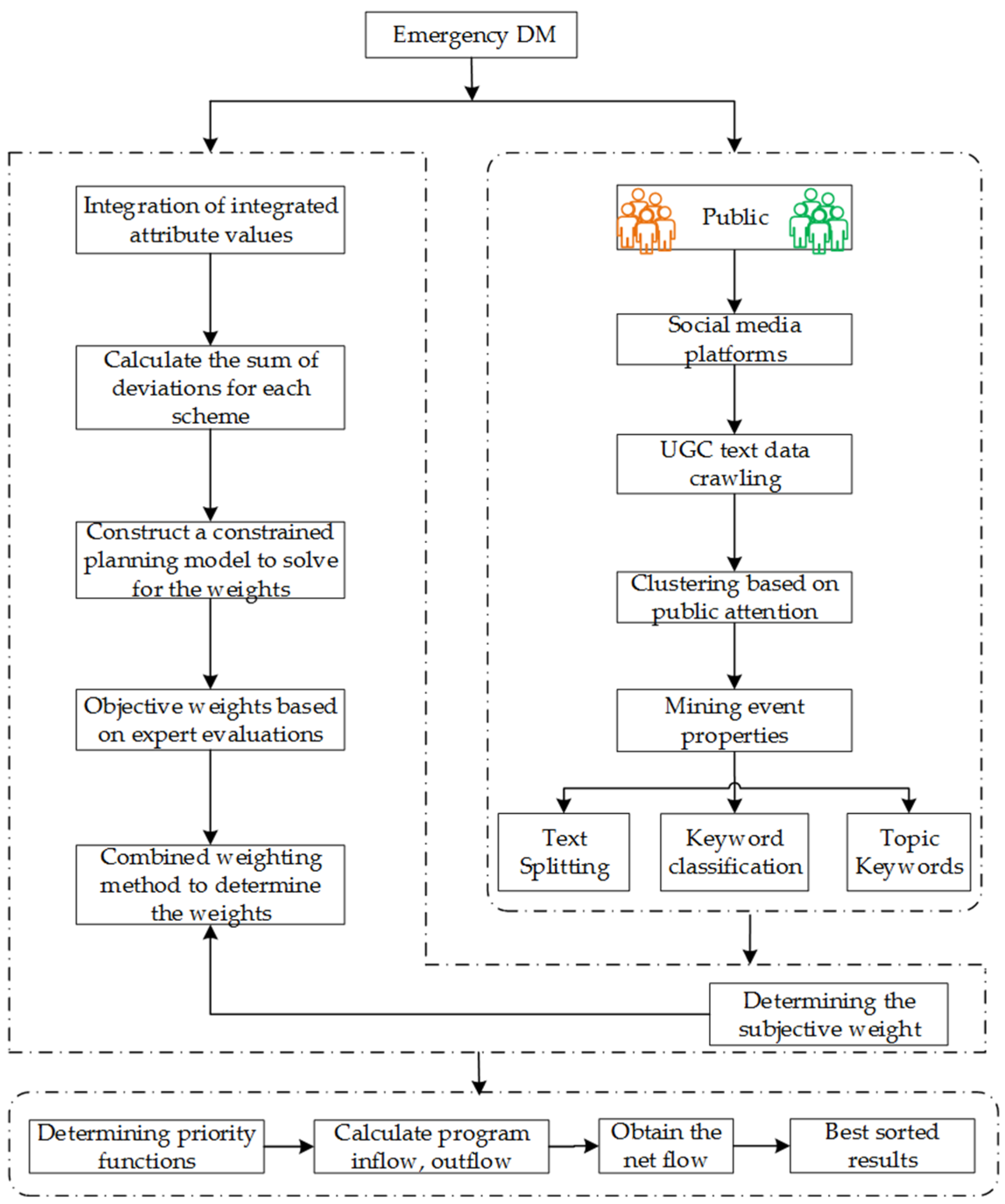
Section 3, we collect public opinions on social media platforms, extract keywords, and explore the attributes of emergency decision-making events as an essential basis for expert evaluation of solutions. Then, we use a combination of subjective and objective weighting models to integrate public opinions with expert decision making by CPT. In Section 4, we provide a specific flow on the GDMD-PROMETHEE algorithm. In Section 5, we verify the validity and feasibility of this paper’s method through the “6–18” Shanghai Petrochemical explosion and compare it with other methods. Meanwhile, a sensitivity analysis was conducted. In Section 6, we present conclusions.

2. Preliminaries

2.1. Probabilistic Linguistic Term Sets

PLTS is one of the most widely used research tool in MAGDM. In this section, we introduce the basic concepts of linguistic term sets (LTSs) and distance measure between them. On this basis, the basic concepts of PLTSs, as well as distance improvement are given.
Definition 1.
[1] Let  S = { s α α = 0 , 1 , 2 , , 2 g , g N + }  be a  L T S , then different language terms may be used. For example, let  S  be the following  L T S : S 9 = s 0 = e x t r e m e l y   l o w , s 1 = v e r y   l o w , s 2 = l o w , s 3 = s l i g h t l y   l o w , s 4 = f a i r , s 5 = s l i g h t l y   h i g h , s 6 = h i g h ,   s 7 = v e r y   h i g h , s 8 = e x t r e m e l y   h i g h ,  s α  satisfies the following conditions:
1. 
The set is ordered:  s α 1 > s α 2 , if  α 1 > α 2 ;
2. 
The negation operator is defined:  n e g ( s α ) = s 2 g α ,
where  s α  can be expressed by the linguistic scale transformation function  f  as:  f ( s α ) = α / 2 g , α  is the subscript of  s α .
Definition 2.
[1] Let  S = { s α α = 0 , 1 , 2 , , 2 g , g N + }  be a  L T S , a PLTS can be defined as:
L ( p ) = L ( k ) ( p ( k ) ) L ( k ) S , p ( k ) 0 , k = 1 , 2 , , # L ( p ) , k = 1 # L ( p ) p ( k ) 1
where  L ( k ) ( p ( k ) )  denotes the associated probability of the set of linguistic terms  L ( k )  with  p ( k ) ;  # L ( p )  denotes the number of linguistic terms in the set of probabilistic linguistic terms.
Note that if k = 1 # L ( p ) p ( k ) = 1 , then we have the complete information of probabilistic distribution of all possible linguistic terms; if k = 1 # L ( p ) p ( k ) 1 , then partial ignorance exists because current knowledge is not enough to provide complete assessment information, which is not rare in practical GDM problems. Especially, k = 1 # L ( p ) p ( k ) = 0 means completely ignorance. Obviously, handling the ignorance of L ( p ) is a crucial work for the use of PLTSs.
Definition 3.
[32] Given a PLTS  L ( p )  with  k = 1 # L ( p ) p ( k ) 1 , then the normalized PLTS  L ˙ ( p )  is defined by:
L ˙ ( p ) = L ( k ) ( p ˙ ( k ) ) L ( k ) S , p ( k ) 0 , k = 1 , 2 , , # L ( p ) , p ˙ ( k ) = p ( k ) / k = 1 # L ( p ) p ( k )
Definition 4.
[11] Let  L ( p )  be a PLTS, the score of  L ( p )  is  E ( L ( p ) ) = s α ¯ , where:
α ¯ = k = 1 # L ( p ) α ( k ) p ( k ) / k = 1 # L ( p ) p ( k )
Definition 5.
[11] The deviation degree of  L ( p )  is:
σ ( L ( p ) ) = k = 1 # L ( p ) ( p ( k ) ( α ( k ) α ¯ ) ) 2 1 / 2 / k = 1 # L ( p ) p ( k )
where  α ( k )  is the subscript of linguistic term  L ( k ) , given two PLTSs  L 1 ( p )  and  L 2 ( p )  then:
(1) 
If  E ( L 1 ( p ) ) > E ( L 2 ( p ) ) , then  L 1 ( p ) L 2 ( p ) ;
(3) 
If  E ( L 1 ( p ) ) < E ( L 2 ( p ) ) , then  L 1 ( p ) L 2 ( p ) ;
(3) 
If  E ( L 1 ( p ) ) = E ( L 2 ( p ) ) , while  σ ( L 1 ( p ) ) < σ ( L 2 ( p ) ) , then  L 1 ( p ) L 2 ( p ) ; while  σ ( L 1 ( p ) ) > σ ( L 2 ( p ) ) , then  L 1 ( p ) L 2 ( p ) ; while  σ ( L 1 ( p ) ) = σ ( L 2 ( p ) ) , then  L 1 ( p ) L 2 ( p ) .

2.2. Distance Measures between PLTSs

PLTSs can more accurately represent qualitative information of DMs in complex linguistic environments. However, existing distance measures may distort the original information and lead to unreasonable results. For this reason, a new generalized hybrid distance based on the classical distance is proposed.
Definition 6.
Let  L 1 ( p ) = L 1 ( k ) ( p 1 ( k ) ) L 1 ( k ) S , p 1 ( k ) 0 , k = 1 , 2 , , # L 1 ( p ) , k = 1 # L 1 ( p ) p 1 ( k ) = 1  and  L 2 ( p ) = L 2 ( k ) ( p 2 ( k ) ) L 2 ( k ) S ,   p 2 ( k ) 0 ,   k = 1 , 2 , , # L 2 ( p ) , k = 1 # L 2 ( p ) p 2 ( k ) = 1  be two PLTSs,  # L 1 ( p ) = # L 2 ( p ) , L 1 ( k )  and  L 2 ( k )  are the  k t h  linguistic terms of  L 1 ( p )  and  L 2 ( p )  respectively,  p 1 ( k )  and  p 2 ( k )  are the probabilities of the  k t h  linguistic terms of  L 1 ( p )  and  L 2 ( p )  respectively,  α 1 ( k )  and  α 2 ( k )  are the subscripts of the linguistic terms corresponding to  L 1 ( k )  and  L 2 ( k ) , respectively, then a new probabilistic linguistic distance based on Reference [33] is defined as:
d ( L 1 ( p ) , L 2 ( p ) ) = 1 2 1 2 k = 1 # L ( p ) p 1 ( k ) p 2 ( k ) + k = 1 # L ( p ) f ( α 1 ( k ) ) p 1 ( k ) k = 1 # L ( p ) f ( α 2 ( k ) ) p 2 ( k )
Definition 7.
[34] Let  L 1 ( p ) = L 1 ( k ) ( p 1 ( k ) ) L 1 ( k ) S , p 1 ( k ) 0 , k = 1 , 2 , , # L 1 ( p ) , k = 1 # L 1 ( p ) p 1 ( k ) = 1  and  L 2 ( p ) = L 2 ( k ) ( p 2 ( k ) ) L 2 ( k ) S ,   p 2 ( k ) 0 ,   k = 1 , 2 , , # L 2 ( p ) , k = 1 # L 2 ( p ) p 2 ( k ) = 1  be two PLTSs,  # L 1 ( p ) = # L 2 ( p ) , L 1 ( k )  and  L 2 ( k )  are the  k t h  linguistic terms of  L 1 ( p )  and  L 2 ( p )  respectively,  p 1 ( k )  and  p 2 ( k )  are the probabilities of the  k t h  linguistic terms of  L 1 ( p )  and  L 2 ( p )  respectively. Then, the extended  H a u s d o r f f  distance is:
d h ( L 1 ( p ) , L 2 ( p ) ) = max k = 1 # L 1 ( p ) 1 2 min k = 1 # L 2 ( p ) f ( α 1 ( k ) ) f ( α 2 ( k ) ) λ + f ( α 1 ( k ) ) p 1 ( k ) f ( α 2 ( k ) ) p 2 ( k ) λ 1 λ
where  f is the linguistic scale function,  λ > 0 , when  λ = 1 , the above Equation(6) is Hamming-Hausdorff distance; when  λ = 2 , the above Equation is Euclidean-Hausdorff distance.
In MAGDM, when the above distances cannot meet the decision needs, this paper creatively introduces probability-related distances to achieve perfect integration with the probabilistic linguistic, and also fully considers the wishes of each decision maker, the new distance is given as follow.
Definition 8.
Let  S = { s α α = 0 , 1 , 2 , , 2 g , g N + }  is an LTS. Let  L 1 ( p ) = L 1 ( k ) ( p 1 ( k ) ) L 1 ( k ) S , p 1 ( k ) 0 , k = 1 , 2 , , # L 1 ( p ) ,   k = 1 # L 1 ( p ) p 1 ( k ) = 1  and  L 2 ( p ) = L 2 ( k ) ( p 2 ( k ) ) L 2 ( k ) S , p 2 ( k ) 0 , k = 1 , 2 , ,   # L 2 ( p ) , k = 1 # L 2 ( p ) p 2 ( k ) = 1  be two  P L T S s , then the generalized hybrid distance between PLTSs is defined as:
D g h ( L 1 ( p ) , L 2 ( p ) ) = η 1 2 1 2 k = 1 # L ( p ) p 1 ( k ) p 2 ( k ) + k = 1 # L ( p ) f ( α 1 ( k ) ) p 1 ( k ) k = 1 # L ( p ) f ( α 2 ( k ) ) p 2 ( k ) λ + ( 1 η ) max k = 1 # L ( p ) 1 2 min k = 1 # L ( p ) f ( α 1 ( k ) ) f ( α 2 ( k ) ) λ + f ( α 1 ( k ) ) p 1 ( k ) f ( α 2 ( k ) ) p 2 ( k ) λ 1 λ
From Equation (7), λ 1 , η 0 , 1 , the generalized hybrid distance combines the generalized probabilistic linguistic distance and the extended Hausdorff distance through the parameter η . The parameter λ can be considered as the expert’s risk attitude, so the proposed distance allows more options for the experts to decide their risk preferences through the parameters.
Theorem 1.
Let  L 1 ( p ) ,  L 2 ( p )  and  L 3 ( p )  be three complete probabilistic linguistic term sets, the three PLTSs are  L 1 ( p ) = L 1 ( k ) ( p 1 ( k ) ) L 1 ( k ) S , p 1 ( k ) 0 , k = 1 , 2 , , # L 1 ( p ) , k = 1 # L 1 ( p ) p 1 ( k ) = 1   L 2 ( p ) = L 2 ( k ) ( p 2 ( k ) ) L 2 ( k ) S , p 2 ( k ) 0 , k = 1 , 2 , , # L 2 ( p ) ,   k = 1 # L 2 ( p ) p 2 ( k ) = 1  and  L 3 ( p ) = L 3 ( k ) ( p 3 ( k ) ) L 3 ( k ) S , p 3 ( k ) 0 , k = 1 , 2 , , # L 3 ( p ) , k = 1 # L 3 ( p ) p 3 ( k ) = 1 , where  L 1 ( k ) ,  L 2 ( k )  and  L 3 ( k )  are the  k t h  linguistic terms in  L 1 ( p ) ,  L 2 ( p )  and  L 3 ( p ) ,  α 1 ( k ) ,  α 2 ( k )  and  α 3 ( k )  are the probabilities of the  k t h  linguistic terms in  L 1 ( p ) ,  L 2 ( p )  and  L 3 ( p )  respectively. Then, the generalized hybrid distance has the following properties:
(1) 
D g h ( L 1 ( p ) , L 2 ( p ) ) 0 ;
(2) 
D g h ( L 1 ( p ) , L 2 ( p ) ) = 0 L 1 ( p ) = L 2 ( p ) ;
(3) 
If  L 1 ( p ) < L 2 ( p ) < L 3 ( p ) ,  then  D g h ( L 1 ( p ) , L 2 ( p ) ) < D g h ( L 1 ( p ) , L 3 ( p ) ) ,  D g h ( L 2 ( p ) , L 3 ( p ) ) < D g h ( L 1 ( p ) , L 3 ( p ) ) .
The proof of Theorem 1 is given in Appendix A.

2.3. Probabilistic Linguistic CPT

2.3.1. Classical CPT

To better retain the true evaluation information of DMs, probabilistic fusion is performed using CPT. CPT [35] is an improved version of prospect theory (PT) [36] to address stochastic dominance proposed by Tversky et al. in 1992, which well explains phenomena such as stochastic dominance, and its measure of the total value of a prospect through a value function and probability weights. The forms are shown as follows:
Combined prospect value:
V ( x ) = i = 0 n v ( x i ) w ( p i )
CPT asserts that there exist a strictly increasing weighted value function v ( x i ) . The value function v ( x i ) is defined on the deviations from a reference point, which represents the behavior of the DMs and can be expressed as follows.
Value function:
v ( x i ) = ( x i b ) ξ , x i b θ ( b x i ) β , x i < b
The key difference between CPT and PT is that the weight function used in CPT is no longer a linear function, but an inverse S-shaped curve, indicating that individual decision makers tend to overestimate the possibility of small probability events and underestimate the possibility of medium and high probability events, so the probability weights of gains and losses are formulated as follows.
Weighting function:
w ( p i ) = w + ( p i ) = p i δ [ p i δ + ( 1 p i ) δ ] 1 / δ , x i b w ( p i ) = p i ε [ p i ε + ( 1 p i ) ε ] 1 / ε , x i < b
where b denotes the reference point; ξ , β are the risk attitude coefficients towards value in the face of gain or loss, ξ , β ( 0 , 1 ) ; θ is the loss aversion coefficient, θ > 1 ; δ , ε are the risk attitude coefficients towards probability weights about gain or loss, δ , ε ( 0 , 1 ) . Combined with Reference [35], it is generally considered to take ξ = β = 0.88 , θ = 2.25 , δ = 0.61 , ε = 0.69 .
Considering the risk preferences of DMs facing gains and losses in real problems, CPT gives a specific form of the value function and a form of decision weights, which let it be combined with probabilistic linguistic as follows. It would be more meaningful to integrate CPT into the practical application of GDM.

2.3.2. The Measures between PLTSs Based on CPT

In order to measure probabilistic linguistic terms more accurately, a new probabilistic linguistic terminology measure is obtained by fusing information based on the value function of the relative reference point variables and the probability weight function.
Definition 9.
[13] The measures between PLTSs based on CPT. The forms are shown as follows:
Score value:
V ( L ( p ) ) = k = 1 # L ( p ) ( v ( α k ) w ( p k ) )
v ( α k ) = ( α k ) ξ , α k 2 θ ( α k ) β , α k < 2
w ( p k ) = p k δ [ p k δ + ( 1 p k ) δ ] 1 / δ , α k 2 p k ε [ p k ε + ( 1 p k ) ε ] 1 / ε , α k < 2
Variance value:
δ ( L ( p ) ) = k = 1 # L ( p ) v ( α k ) E ( α k ) 2 w ( p k ) 1 / 2
where  α k  is the subscript of  S ,  S = { s α α = 0 , 1 , 2 , , 2 g , g N + } , here  α k = 0 , 1 , 2 , 3 , 4 ,  p k δ  is the probability of  α k .
CPT not only analyzes the risk psychological factors of human in the decision making process. It also considers the value function and probability weight function of the relative reference point variables, which makes up for the shortcomings of PT.

3. Comprehensive Assignment Method to Determine Attribute Weights

3.1. Obtain Objective Weights Based on Social Media Data Mining

3.1.1. Data Clustering of Large Groups Based on Data Attention

The typical way for the public to express their feelings, views, opinions, etc., is through behavior [7]. Public behavior data are mainly divided into operational (interaction) behavior data and content behavior data. The first refers to published texts, while the second mainly involves data on public commenting, liking, and retweeting behaviors. This study uses a Python-based crawler technique to obtain the raw microblog data, which mainly includes the blogger’s ID screen name, blog post text, posting time, number of likes, number of retweets, number of comments, and others. The flow of obtaining event attributes and attribute weights are shown in Figure 1.
First, use Python-based crawler technique to collect a large amount of information about user behavior on social media networks. Each piece of data can be denoted as D = ( U G C , A N , C N , R N , F N , F S N ) . A N , C N , R N , F N , F S N and U G C represent the number of likes, comments, retweets, followers and tweet texts (user-generated content), respectively. Then, each text data is pre-processed using the Python natural language processing package, including word separation, cleaning, lexical annotation, and entity word recognition. Finally, after the data pre-processing, the k -means clustering algorithm is chosen to classify the data based on the public attention level.
In order to obtain the optimal number of clusters in the process of cluster analysis and ensure more scientific results of data classification, the elbow method and the contour coefficient method are generally adopted to determine the optimal value. In contrast, the optimal k value determined by the contour coefficient method is not necessarily optimal. Sometimes it needs to be obtained with the aid of S S E ; therefore, in this paper, we first consider using the elbow method of Equation (13) to determine the optimal number of clusters. The core index of the elbow method is sum of the squared errors S S E :
S S E = i = 1 k p C i p m i 2
where C i is the i t h cluster, p is the sample points in C i , m i is the center of mass of C i (the mean of all samples in C i ) and S S E is the clustering error of all models, representing the good or lousy clustering effect. The core idea of the elbow method is that as the number of clusters k increases, the sample division will be finer, and the degree of aggregation of each cluster will gradually increase. Then, S S E will naturally become smaller gradually.
Each dataset is obtained after classifying the data containing multiple data objects. Based on the information of each data item in the dataset, the attention coefficient of the dataset is calculated, where D S i ( A N ) , D S i ( C N ) , D S i ( R N ) , D S i ( F N ) and D S i ( F S N ) denote the average number of likes, average number of comments, the average number of retweets, the average number of followers and average number of fans of the i t h dataset, respectively. The denominator n i denotes the number of data in the dataset, and the attention factor γ i formula [7] is as follows:
γ i = a D S i ( A N ) + c D S i ( C N ) + r D S i ( R N ) + f D S i ( F N ) + s D S i ( F S N ) i = 1 t a D S i ( A N ) + c D S i ( C N ) + r D S i ( R N ) + f D S i ( F N ) + s D S i ( F S N )
where D S i ( A N ) = D i j D S i A N i j n i , D S i ( C N ) = D i j D S i C N i j n i , D S i ( R N ) = D i j D S i R N i j n i , D S i ( F N ) = D i j D S i F N ij n i ,
D S i ( F S N ) = D i j D S i F S N i j n i
A linear programming model is developed to maximize the influence of the data, where Z is the influence of the data, A , B , C , D , E determine the number of likes, comments, retweets, followers and followers of the data, respectively, and a , c , r , f , s mean the weights of each index, respectively. If the influence of each factor is equal, find the data’s maximum influence and the indicator’s weight as follows:
M a x Z = A a + B c + C r + D f + E s s . t . A a B c = 0 A a C r = 0 A a D f = 0 D f E s = 0 a + c + r + f + s = 1 a , c , r , f , s 0
Obtain the weights of each indicator by solving this linear programming model. The method of using the model to determine the indicator weights is more objective than others. It can effectively avoid the risk of decision making caused by experts’ subjective determination of the indicator weights, which makes the method to be more scientific and applicable.

3.1.2. Obtain Attributes and Weights

Once an emergency breaks out, the microblogging platform forms real-time hot topics, and the text of microblogs representing public views proliferates to form a significant data stream. Term frequency–inverse document frequency (TF-IDF) is a widely used keyword extraction technique in the field of data miningand evolved from IDF which is proposed by Sparck Jones [37,38] with heuristic intuition. It is a common weighting technique used in information retrieval and text mining to evaluate the importance of a word in a document collection by considering the word frequency and the inverse document frequency to determine the weight of the keyword.
The specific steps of the algorithm are as follows:
Step1.
Calculate the word frequency.
Word frequency is the number of times a word appears in an article. The word frequency is standardized to facilitate the comparison of different articles and explained the difference in length of the articles.
tf i j = n i , j k n k , j
where n i , j is the number of occurrences of the word in a document d j , and the denominator is the sum of the occurrences of all words in the document d j .
Step2.
Calculate inverse document frequency as
i d f i = log D j : t i d j
where D is the total number of documents in the corpus and j : t i d j denotes the number of documents containing the word t i . If the word is not in the corpus, it will result in a denominator of 0. Therefore, in general, 1 + j : t i d j is used, i.e.,
Step3.
Calculate TF-IDF as
T F I D F = T F × I D F
Finally, the weights of public attributes are obtained by combining the attention coefficients γ i of the dataset, and the standard decision attribute weights are obtained after normalization. Combining the attention coefficients obtained by Equation (16), the weights of public attributes are obtained and normalized to get the standard decision attribute weights.

3.2. Determine Expert Subjective Weights Based on Disparity Maximization

In this paper, the idea of disparity maximization is used to determine the weight of each decision. Wang [34] proposed the maximum deviation method to deal with MADM problems with numerical information [39]. For the MAGDM problem, if the variance of a DMs’ attribute evaluation value is more minor for all solutions, it means that the DMs’ decision plays a smaller role in the ranking of solutions; conversely, if the variance of a DMs’ attribute evaluation value is larger for all solutions, it means that the DMs’ decision plays a larger role in the ranking of solutions, and the DMs should be given a larger weight at this time. This method can motivate DMs’ to make an objective and reasonable evaluation of known solutions.
Suppose all the attribute indicators in this paper are benefit-based indicators, which do not need to be normalized.
The specific steps are as follows:
Step1.
Obtain the decision-making matrix R = ( r i j ) n × m from the expert e k . The evaluated value of the alternative A i on C j can be expressed as v i j k , which is expressed in PLTS.
Step2.
Based on the maximum deviation method, construct the objective function:
M a x F ( w j ) = j = 1 m w j i = 1 n k = 1 , k i n D ( r i j , r k j ) s . t j = 1 m w j 2 = 1 w j 0 , j = 1 , 2 , , m
Solve this optimal model as a Lagrange function:
F ( w j , λ ) = j = 1 m w j i = 1 n k = 1 , k i n D ( r i j , r k j ) + λ 2 j = 1 m w j 2 1
Derive the partial derivative of Equation (23) and let:
F ( w j , λ ) w j = i = 1 n k = 1 , k i n D ( r i j , r k j ) + λ w j = 0 F ( w j , λ ) λ = j = 1 m w j 2 1 = 0
Find the optimal solution:
w j = i = 1 n k = 1 , k i n D ( r i j , r k j ) i = 1 n k = 1 , k i n D ( r i j , r k j ) 2
Step3.
Normalize the weights as
w j = w j j = 1 m w j = i = 1 n k = 1 , k i n D ( r i j , r k j ) j = 1 m i = 1 n k = 1 , k i n D ( r i j , r k j )

3.3. Combined Weights

Let w i j k denotes the combined weight of expert e k for alternative A i on the attribute C j , by combining the subjective weight w j with the objective weight w i j k :
w i j k = α W i j k + β w j
where α , β are the linear expression coefficients of the combined weights and satisfy 0 α , β 1 , α + β = 1 , i = 1 , 2 , , n , j = 1 , 2 , , m , k = 1 , 2 , , n . When α = 0 and β = 1 only subjective weights are considered in GDM; when α = 1 and β = 0 , only objective weights are considered in GDM.

4. GDMD-PROMETHEE Algorithm Based on CPT

This section provides a new extended PROMETHEE using probabilistic linguistic information, namely the GDMD-PROMETHEE method, to evaluate multi-criterion GDM. Let A i ( i = 1 , 2 , , n ) be the alternative, C j ( j = 1 , 2 , , m ) be the criterion mined through social media, and E k ( k N + , k 20 ) be the decision-making experts from relevant fields. Based on a two-by-two comparison of A i ( i = 1 , 2 , , n ) , A i ( i = 1 , 2 , , n ) are ranked by GDMD-PROMETHEE. The flow chart of GDMD-PROMETHEE is shown in Figure 2.
Based on the above analysis, the specific steps of GDMD-PROMETHEE are as follows:
Step1.
Combine big data network behavior data to mine event keywords, obtain event evaluation criteria, and use TF-IDF technique to find the subjective weights of event attributes.
Step2.
Solve the objective weights of experts using Equations (22)–(26) to determine the comprehensive weights w i j k .
Step3.
Combine Equations (12)–(14) to fuse the probabilistic linguistic evaluation information into specific real values to obtain the fused initial evaluation matrix.
Step4.
Combine the integrated weights with the initial evaluation matrix to obtain the group evaluation matrix V = [ v i j l ] n × n .
Step5.
Calculate the priority indices of two solutions under different attributes as
r j k = l = 1 t h = 1 l v j l v k h 1 2 l = 1 t v j l v k l , j , k = 1 , 2 , , n
r k j = l = 1 t h = 1 l v j l v k h 1 2 l = 1 t v j l v k l , j , k = 1 , 2 , , n
Step6.
Construct the dominance matrix for pairwise comparisons between solutions, when the solution is compared with itself, then the dominance ratio is 0.5, and the rest of the cases satisfy r j k + r k j = 1 .
R = [ r j k ] n × n = A 1 A 2 A n A 1 A 2 A n [ r 11 r 21 r n 1 r 12 r 22 r n 2 r 1 n r 2 n r n n ]
Step7.
From Equation (33), the net flow value ϕ ( i ) of each solution is obtained, and the larger ϕ ( i ) is, the better the solution is. The outflow ϕ + ( A j ) of A j indicates the extent to which A j outperforms the other ( n 1 ) scenarios in the set, and the larger the outflow ϕ + ( A j ) , the better A j is. The inflow indicates the extent to which the other ( n 1 ) solutions in the solution set out perform A j . The smaller ϕ - ( A j ) , the better A j is. The formulas are as follows:
ϕ + ( A j ) = 1 n k = 1 n r j k , j = 1 , 2 , n .
ϕ - ( A j ) = 1 n k = 1 n r k j , j = 1 , 2 , n .
ϕ ( A j ) = 1 n k = 1 n r j k , j = 1 , 2 , n .
As one of the most widely used ranking methods in MAGDM, PROMETHEE is convenient and flexible to use due to its ease of understanding. Based on this paper, we propose the GDMD-PROMETHEE algorithm based on CPT.

5. Case Study

5.1. Case Background

Take the Shanghai Petrochemical explosion on 18 June 2022 as an example to verify the method’s feasibility in this paper. At 4:28 pm on 18 June 2022, the chemical department of Shanghai Petrochemical caught fire, and the fireball shot up to the sky with explosions in many places. In order to protect the basic life safety of the public and ensure the emergency command carries out the coordination work quickly. After consulting professional information, four alternatives were identified, and 20 emergency decision-making experts from firefighting, medical, chemical and other related departments evaluated each option in terms of attributes, and the four options were:
A 1  
Timely understanding of the destruction of the surrounding traffic, communications, power supply, water supply and other facilities, the deployment of drones to draw a 360-degree panoramic map of the explosion site, survey the hidden fire point, determine the rescue route, organize a rescue, reasonable arrangement of firefighting and rescue forces, to protect the safety of people and property. After the fire is extinguished, the organization will organize forces to seal the leak point for repair work to ensure the successful completion of the anti-disaster work.
A 2  
After the fire, the attacking team was sent to the scene to detect the gas, strengthen the personal protection of rescue personnel and quickly rescue the trapped personnel. Moreover, take the initial battle to control the fire, cooling, and explosion suppression tactical measures, synchronization of multiple fire points and surrounding storage tanks, devices for cooling protection, to prevent heating, pressure and cause secondary fire explosion.
A 3  
Immediately after discovering the leaking device, stop transmission, close the cut-off valves on both sides of the pipeline leak point, take necessary protective measures for other pipelines near the leaking pipeline and, at the same time, be alert to electricity leakage, highly toxic and highly corrosive substances. Make every effort to help the injured, and take isolation, caution and evacuation measures to avoid extraneous personnel from entering the danger area. Activate the environmental emergency plan and arrange to test the surrounding air and water quality.
A 4  
To avoid the secondary explosion of unknown hazardous materials, suspend large-scale firefighting, dispatch the chemical prevention regiment, nuclear, biological and chemical emergency rescue team to search and rescue the scene in depth, and sample burning materials, according to the composition of burning materials selected to correspond to the firefighting methods. Take anti-leakage and anti-proliferation control measures to prevent the spread of fire. After the fire was controlled, protective burning was implemented.
Using Python to crawl microblog data, keywords such as Shanghai petrochemical fire accident has set up an investigation team, Shanghai petrochemical fire information, aerial photography of Shanghai petrochemical fire scene, Shanghai petrochemical fire latest progress. A total of 1200 pieces of data were extracted; each piece of data consisted of D = ( U G C , A N , C N , R N , F N , F S N ) pieces of data. Data Availability Statement: The data of this study are available from the authors upon request. Relevant data are available from the “Wei Bo” website (https://weibo.com/ (accessed on 18 June 2022)).
After cleaning and filtering the data, about 400 pieces of valid data were retained and used to generate a word cloud map as Figure 3.

5.2. Data Analysis

Step1.
After data pre-processing, the number of likes, comments and retweets of the data as distance measures, the k -means clustering algorithm is applied to complete the behavioral big data clustering based on public attention, as the number of categories of classification increases, the decline of S S E will plummet and then level off as the k -value continues to increase, the elbow method is to select that the inflection point, so as shown in Figure 4, k = 3 should be selected.
After converting the distances into probability distributions using Gaussian distributions in high-dimensional space, determining the optimal number of clusters k = 3 T-SNE Python by reducing the 3D features of high-dimensional data to 2D visualization. The different colors in the diagram represent a small group, and each small group is a category. Blue, green and red represent D S 1 , D S 2 and D S 3 at low dimension, respectively. It makes it possible to maintain the information they carry in high-dimensional, even in low-dimensional space, as shown in Figure 5.
Using the linear programming model established by Equation (18), the weights of the resulting indicators are calculated as shown in Table 1, and the concern coefficients for each data set are obtained according to Equation (16), which is presented in Table 2 as follows:
In this paper, the words with high TF-IDF values are selected as keywords for the subsequent extensive data use Jieba Python. In order to facilitate the subsequent analysis, some words that are not highly related to the emergency event and have dark themes are deleted. For example, the words that are not related to the explosion are “original”, “good night”, “takeout”, etc. Based on the above analysis, the emergency decision guidelines and their corresponding keywords considering the topic of public concern for mega emergencies are shown in Table 3. Determine four attributes C j = C 1 , C 2 , C 3 , C 4 , where C 1 is “emergency response”, including emergency response, control, preplanning, etc. C 2 is “fire suppression and derivative disaster control”, including fire, burning, etc. C 3 is “site and surrounding environment detection”, including photography, smoke, pollution, etc. C 4 is “casualty and rescue”, including injury, death, rescue, etc. The corresponding weights of each attribute are w j = w 1 , w 2 , w 3 , w 4 = 0.250 , 0.204 , 0.174 , 0.372 .
Step2.
The objective weights are obtained using Equations (22)–(26) as in Table 4, and there is no difference in the deviation values of experts e 7 , e 9 and e 15 , so the weights are assigned to 0.
Step3.
According to Equation (27), the integrated weights are calculated, here let α = β = 0.5 , and Table 5 is obtained.
Step4.
Combined with the four attributes identified in Table 3, the experts gave the ratings in terms of the four attributes under the five-grain language S = s 0 , s 1 , s 2 , s 3 , s 4 = {very low, low, fair, high, very high}, due to space issues, the rating matrices of the top two experts are listed, as shown in Table 6 and Table 7 below.
The evaluation information was fused based on the cumulative Equations (11) to (13), then obtain the initial evaluation matrix transformed into real values, and the results are shown in Table 8, additional complementary results are in Appendix B.
Step5.
The weights were combined with the evaluation information to obtain the normalized group evaluation matrix, as shown in Table 9.
Step6.
The advantage ratios between the two solutions are calculated using Equations (29)–(30), as shown in Table 10.
Step7.
By calculating the inflow, outflow and net flow for each scenario, the net flow for each scenario is derived and the results are shown in Table 11.
By comparing the size of the net flow, the final program ranking: A 2 A 1 A 3 A 4 , that is, the choice of program A 2 : After the fire, the attack team was sent to the scene to detect the gas, strengthen the personal protection of rescue personnel and quickly rescue the trapped personnel. Take the initial battle to control the fire, cooling and explosion suppression tactical measures, simultaneous cooling protection of multiple fire points and surrounding tanks and devices to prevent heating and pressure and cause a fire secondary explosion.

5.3. Sensitivity Analysis

5.3.1. Ranking Results under Different Parameters by the Same Decision Method

For sensitivity analysis, the effect of different sizes of α and β under the combined weights on the ranking results was investigated, where the coefficient α represents the percentage of objective weights and coefficient β represents the percentage of subjective weights. The results are shown in Table 12.
As can be seen from Table 12, the optimal solution is A 1 except when α = 1 , β = 0 (i.e., only objective weights are considered); in all other cases, the solution ranking results maintain good consistency, i.e., A 2 A 1 A 3 A 4 . It shows that the goodness of the schemes is not affected by the large fluctuations of the parameters regardless of the cases, and the comparison with the method in Reference [40] confirms that the GDMD-PROMETHEE method combining generalized probability distance and Hausdorff is more stable. By observing the scores obtained in Figure 6 and Figure 7, it can be seen that the scores of scenarios and schemes are relatively close under each parameter, but A 2 is the best and A 4 is the worst, and it is obviously undesirable to consider only the objective weights.

5.3.2. Comparison the Ranking Results of Different Decision Methods

To verify the validity and feasibility of the model in this paper, the methods of literature [40,41] and TOPSIS analysis were selected to make a comparison of the results, as shown in the following table.
(1)
By observing Table 13, it can be obtained that the result of PROMETHEE ranking based on the literature [41] is A 3 A 2 A 1 A 4 , which is different from the result of this paper. The main reason is that this paper considers the weights of individual decision experts. The literature [41] only assigns the same average weight to decision groups. The method of assigning expert weights based on the maximum deviation value extracted from the evaluation of individual decision experts in this paper is more consistent with the individual decision risk levels and attitudes of experts compared to the simple average weight.
(2)
As can be seen from Table 13, the PROMETHEE method based on CPT has the same ranking results as the traditional TOPSIS method and the literature [40]. Combined with Figure 8, it can be seen that the comparative analysis results of the first three methods are relatively consistent, i.e., the best solution A 2 , the worst solution A 4 , which further verifies the validity and reasonableness of the method in this paper.

6. Conclusions

In this paper, we study emergency decision making in the social media environment in the era of big data and use probabilistic language methods to cluster the decision results. Compared with traditional GDM, this paper not only extracts event attributes from public information but also combines public opinion with weights, which effectively and quickly incorporates public opinion into the final decision information and helps to grasp the actual development of the emergency. A new generalized extended hybrid distance is proposed to determine the objective weights of each decision expert based on the expert decision information using the maximum difference method. The decision weight coefficients are used to adjust the proportion of subject, object, and view weights to obtain the total weights. The influence on the decisions made under the weights of different perspectives is studied. Using the CPT to combine the probabilistic linguistic evaluation information with the total weights and finally taking the Shanghai Petrochemical “6.18” explosion as an example, the rationality and feasibility of GDMD-PROMETHEE method are verified. Combining the external influences of public opinion with the influence of each public member in decision making needs to be studied further in future. In addition, the dynamic change process of experts’ opinion can be described so that the decision-making process is closer to the actual situation and the decision results are more scientific.

Author Contributions

Conceptualization, J.W. and S.L.; methodology, J.W.; software, S.L.; validation, S.L. and X.Z.; formal analysis, J.W. and S.L.; investigation, X.Z.; resources, J.W.; data curation, X.Z.; writing—original draft preparation, J.W. and S.L.; writing—review and editing, J.W. and S.L.; visualization, S.L.; supervision, S.L.; project administration, S.L.; funding acquisition, J.W. All authors have read and agreed to the published version of the manuscript.

Funding

This study was funded by the Projects of Natural Science Research in Anhui Colleges and Universities (2020jyxm0335, KJ2021JD20), the Projects of College Mathematics Teaching Research and Development Center (CMC20210414), the Projects of Natural Science Research in Anhui Jianzhu University (2021xskc01) (2020jy62) (2020szkc01) (HYB20220179).

Institutional Review Board Statement

Not applicable.

Informed Consent Statement

Not applicable.

Data Availability Statement

The data used to support the findings of this study can be used by anyone without prior permission of the authors by just citing this article.

Conflicts of Interest

The authors declare no conflict of interests regarding the publication for the paper.

Appendix A

Proof must be formatted as follows: it is easy to verify properties 1 and 2 in Theorem 1. Proof of property 3 is shown in the following formula:
D g h ( L 1 ( p ) , L 2 ( p ) ) = η 1 2 1 2 k = 1 # L ( p ) p 1 ( k ) p 2 ( k ) + k = 1 # L ( p ) f ( α 1 ( k ) ) p 1 ( k ) k = 1 # L ( p ) f ( α 2 ( k ) ) p 2 ( k ) λ + ( 1 η ) max k = 1 # L ( p ) 1 2 min k = 1 # L ( p ) f ( α 1 ( k ) ) f ( α 2 ( k ) ) λ + f ( α 1 ( k ) ) p 1 ( k ) f ( α 2 ( k ) ) p 2 ( k ) λ 1 λ D g h ( L 1 ( p ) , L 3 ( p ) ) = η 1 2 1 2 k = 1 # L ( p ) p 1 ( k ) p 3 ( k ) + k = 1 # L ( p ) f ( α 1 ( k ) ) p 1 ( k ) k = 1 # L ( p ) f ( α 3 ( k ) ) p 3 ( k ) λ + ( 1 η ) max k = 1 # L ( p ) 1 2 min k = 1 # L ( p ) f ( α 1 ( k ) ) f ( α 3 ( k ) ) λ + f ( α 1 ( k ) ) p 1 ( k ) f ( α 3 ( k ) ) p 3 ( k ) λ 1 λ
As L 1 ( p ) < L 2 ( p ) < L 3 ( p ) and Definition 2, max f ( α 1 ( k ) ) < min f ( α 2 ( k ) ) , max f ( α 2 ( k ) ) < min f ( α 3 ( k ) ) , Given that all three are complete sets of probabilistic linguistic terms, it follows that:
k = 1 # L ( p ) f ( α 1 ( k ) ) p 1 ( k ) ( max f ( α 1 ( k ) ) ) × k = 1 # L ( p ) p 1 ( k ) k = 1 # L ( p ) f ( α 1 ( k ) ) p 1 ( k ) max f ( α 1 ( k ) ) ( min f ( α 2 ( k ) ) ) × k = 1 # L ( p ) p 2 ( k ) k = 1 # L ( p ) f ( α 2 ( k ) ) p 2 ( k ) ( max f ( α 2 ( k ) ) ) × k = 1 # L ( p ) p 2 ( k ) min f ( α 2 ( k ) ) k = 1 # L ( p ) f ( α 2 ( k ) ) p 2 ( k ) max f ( α 2 ( k ) ) k = 1 # L ( p ) f ( α 3 ( k ) ) p 3 ( k ) ( min f ( α 3 ( k ) ) ) × k = 1 # L ( p ) p 3 ( k ) k = 1 # L ( p ) f ( α 3 ( k ) ) p 3 ( k ) min f ( α 3 ( k ) )
Combining the above Equation gives:
k = 1 # L ( p ) f ( α 1 ( k ) ) p 1 ( k ) max f ( α 1 ( k ) ) < min f ( α 2 ( k ) ) k = 1 # L ( p ) f ( α 2 ( k ) ) p 2 ( k ) max f ( α 2 ( k ) ) < min f ( α 3 ( k ) ) k = 1 # L ( p ) f ( α 3 ( k ) ) p 3 ( k ) k = 1 # L ( p ) f ( α 1 ( k ) ) p 1 ( k ) < k = 1 # L ( p ) f ( α 2 ( k ) ) p 2 ( k ) < k = 1 # L ( p ) f ( α 3 ( k ) ) p 3 ( k ) 0 < k = 1 # L ( p ) f ( α 2 ( k ) ) p 2 ( k ) k = 1 # L ( p ) f ( α 1 ( k ) ) p 1 ( k ) < k = 1 # L ( p ) f ( α 3 ( k ) ) p 3 ( k ) k = 1 # L ( p ) f ( α 1 ( k ) ) p 1 ( k ) k = 1 # L ( p ) f ( α 1 ( k ) ) p 1 ( k ) k = 1 # L ( p ) f ( α 2 ( k ) ) p 2 ( k ) = k = 1 # L ( p ) f ( α 2 ( k ) ) p 2 ( k ) k = 1 # L ( p ) f ( α 1 ( k ) ) p 1 ( k ) < k = 1 # L ( p ) f ( α 3 ( k ) ) p 3 ( k ) k = 1 # L ( p ) f ( α 1 ( k ) ) p 1 ( k ) = k = 1 # L ( p ) f ( α 1 ( k ) ) p 1 ( k ) k = 1 # L ( p ) f ( α 3 ( k ) ) p 3 ( k ) 1 2 k = 1 # L ( p ) p 1 ( k ) p 2 ( k ) = 1 2 k = 1 # L 1 ( p ) p 1 ( k ) p 2 ( k ) + 1 2 k = 1 # L 2 ( p ) p 1 ( k ) p 2 ( k ) + 1 2 k = 1 # L 3 ( p ) p 1 ( k ) p 2 ( k ) = 1 2 k = 1 # L 1 ( p ) p 1 ( k ) + 1 2 k = 1 # L 2 ( p ) p 2 ( k ) + 0 = 1 1 2 k = 1 # L ( p ) p 1 ( k ) p 2 ( k ) = 1 2 k = 1 # L ( p ) p 1 ( k ) p 3 ( k ) = 1
Thus:
1 2 1 2 k = 1 # L ( p ) p 1 ( k ) p 2 ( k ) + k = 1 # L ( p ) f ( α 1 ( k ) ) p 1 ( k ) k = 1 # L ( p ) f ( α 2 ( k ) ) p 2 ( k ) = 1 2 1 2 k = 1 # L ( p ) p 1 ( k ) p 3 ( k ) + k = 1 # L ( p ) f ( α 1 ( k ) ) p 1 ( k ) k = 1 # L ( p ) f ( α 2 ( k ) ) p 2 ( k ) < 1 2 1 2 k = 1 # L ( p ) p 1 ( k ) p 3 ( k ) + k = 1 # L ( p ) f ( α 1 ( k ) ) p 1 ( k ) k = 1 # L ( p ) f ( α 3 ( k ) ) p 3 ( k )
The same can be proven:
f ( α 1 ( k ) ) f ( α 2 ( k ) ) < f ( α 1 ( k ) ) f ( α 3 ( k ) ) , f ( α 1 ( k ) ) p 1 ( k ) f ( α 2 ( k ) ) p 2 ( k ) < f ( α 1 ( k ) ) p 1 ( k ) f ( α 3 ( k ) ) p 3 ( k ) f ( α 1 ( k ) ) f ( α 2 ( k ) ) λ < f ( α 1 ( k ) ) f ( α 3 ( k ) ) λ f ( α 1 ( k ) ) p 1 ( k ) f ( α 2 ( k ) ) p 2 ( k ) λ < f ( α 1 ( k ) ) p 1 ( k ) f ( α 3 ( k ) ) p 3 ( k ) λ min k = 1 # L ( p ) f ( α 1 ( k ) ) f ( α 2 ( k ) ) λ + f ( α 1 ( k ) ) p 1 ( k ) f ( α 2 ( k ) ) p 2 ( k ) λ < min k = 1 # L ( p ) f ( α 1 ( k ) ) f ( α 2 ( k ) ) λ + f ( α 1 ( k ) ) p 1 ( k ) f ( α 3 ( k ) ) p 3 ( k ) λ max k = 1 # L ( p ) 1 2 min i = 1 t f ( α 1 ( k ) ) f ( α 2 ( k ) ) λ + f ( α 1 ( k ) ) p 1 ( k ) f ( α 2 ( k ) ) p 2 ( k ) λ 1 λ < max k = 1 # L ( p ) 1 2 min j = 1 m f ( α 1 ( k ) ) f ( α 3 ( k ) ) λ + f ( α 1 ( k ) ) p 1 ( k ) f ( α 3 ( k ) ) p 3 ( k ) λ 1 λ .
Combining the above equations, when λ = 1 or λ = 2 , yields the following Equation.
1 2 1 2 k = 1 # L ( p ) p 1 ( k ) p 2 ( k ) + 1 2 g k = 1 # L ( p ) f ( α 1 ( k ) ) p 1 ( k ) k = 1 # L ( p ) f ( α 2 ( k ) ) p 2 ( k ) λ 1 2 1 2 k = 1 # L ( p ) p 1 ( k ) p 3 ( k ) + 1 2 g k = 1 # L ( p ) f ( α 1 ( k ) ) p 1 ( k ) k = 1 # L ( p ) f ( α 3 ( k ) ) p 3 ( k ) λ , max k = 1 # L ( p ) 1 2 min k = 1 # L ( p ) f ( α 1 ( k ) ) f ( α 2 ( k ) ) λ + f ( α 1 ( k ) ) p 1 ( k ) f ( α 2 ( k ) ) p 2 ( k ) λ max k = 1 # L ( p ) 1 2 min k = 1 # L ( p ) f ( α 1 ( k ) ) f ( α 3 ( k ) ) λ + f ( α 1 ( k ) ) p 1 ( k ) f ( α 3 ( k ) ) p 3 ( k ) λ , η 1 2 1 2 k = 1 # L ( p ) p 1 ( k ) p 2 ( k ) + k = 1 # L ( p ) f ( α 1 ( k ) ) p 1 ( k ) k = 1 # L ( p ) f ( α 2 ( k ) ) p 2 ( k ) λ + ( 1 η ) max k = 1 # L ( p ) 1 2 min k = 1 # L ( p ) f ( α 1 ( k ) ) f ( α 2 ( k ) ) λ + f ( α 1 ( k ) ) p 1 ( k ) f ( α 2 ( k ) ) p 2 ( k ) λ 1 λ η 1 2 1 2 k = 1 # L ( p ) p 1 ( k ) p 3 ( k ) + k = 1 # L ( p ) f ( α 1 ( k ) ) p 1 ( k ) k = 1 # L ( p ) f ( α 3 ( k ) ) p 3 ( k ) λ + ( 1 η ) max k = 1 # L ( p ) 1 2 min k = 1 # L ( p ) f ( α 1 ( k ) ) f ( α 3 ( k ) ) λ + f ( α 1 ( k ) ) p 1 ( k ) f ( α 3 ( k ) ) p 3 ( k ) λ 1 λ D g h ( L 1 ( p ) , L 2 ( p ) ) D g h ( L 1 ( p ) , L 3 ( p ) )
Ditto for easy proof: D g h ( L 2 ( p ) , L 3 ( p ) ) D g h ( L 1 ( p ) , L 3 ( p ) ) . Thus, Theorem 1 is proved.

Appendix B

All the results of Table 8 are as follows:
Table A1. The complete evaluation matrix.
ExpertAlternative C 1 C 2 C 3 C 4
e 1 A 1 3.3870.0003.387−2.250
A 2 2.6291.840−2.2502.629
A 3 3.387−2.2502.6291.840
A 4 0.0002.629−2.2503.387
e 2 A 1 2.6292.6293.3872.629
A 2 3.3873.3873.3873.387
A 3 3.3873.3873.3873.387
A 4 3.3873.3872.6293.387
e 3 A 1 −2.250−2.2501.8401.840
A 2 1.8401.8401.8401.840
A 3 2.6292.6292.6292.629
A 4 −2.250−2.2501.8401.840
e 4 A 1 2.6292.6293.3872.629
A 2 3.3873.3871.8403.387
A 3 2.6292.6292.6292.629
A 4 1.8403.3872.629−2.250
e 5 A 1 2.6293.3873.3873.387
A 2 3.3872.6293.3872.629
A 3 3.3872.6292.6293.387
A 4 3.3873.3873.3872.629
e 6 A 1 2.6291.8401.8402.629
A 2 2.6293.3871.8403.387
A 3 2.6293.3873.3871.840
A 4 1.8403.3873.387−2.250
e 7 A 1 3.3873.3873.3873.387
A 2 3.3873.3873.3873.387
A 3 3.3873.3873.3873.387
A 4 3.3873.3873.3873.387
e 8 A 1 3.3873.3873.3873.387
A 2 3.3873.3873.3872.629
A 3 3.3873.3873.3873.387
A 4 3.3872.6292.6292.629
e 9 A 1 1.8401.8401.8401.840
A 2 1.8401.8401.8401.840
A 3 3.3873.3873.3873.387
A 4 0.0000.0000.0000.000
e 10 A 1 2.6292.6291.8401.840
A 2 3.3873.3871.8402.629
A 3 3.3873.3873.3873.387
A 4 2.6293.3872.6293.387
e 11 A 1 2.6292.6291.8402.629
A 2 3.3872.6292.6292.629
A 3 2.6292.6291.8402.629
A 4 2.6292.6292.6292.629
e 12 A 1 −2.250−2.2501.8400.000
A 2 2.629−2.2501.8403.387
A 3 2.6292.6292.6292.629
A 4 2.6292.6291.8402.629
e 13 A 1 2.629−2.2500.000−2.250
A 2 2.6291.840−2.2502.629
A 3 3.3872.6292.6292.629
A 4 1.8402.6290.0001.840
e 14 A 1 2.6291.8402.6291.840
A 2 1.8402.6292.6291.840
A 3 2.6292.6292.6292.629
A 4 −2.2501.840−2.250−2.250
e 15 A 1 2.6292.6292.6292.629
A 2 2.6292.6292.6292.629
A 3 2.6292.6292.6292.629
A 4 2.6292.6292.6292.629
e 16 A 1 2.6291.8403.3872.629
A 2 1.8403.3873.3873.387
A 3 2.6293.3872.6292.629
A 4 2.6293.3872.6292.629
e 17 A 1 1.8402.6292.6292.629
A 2 2.6291.840−2.250−2.250
A 3 3.3872.629−2.250−2.250
A 4 −2.250−2.250−2.250−2.250
e 18 A 1 2.6293.3873.3873.387
A 2 3.3873.3872.6292.629
A 3 3.3873.3872.6292.629
A 4 2.6293.3873.3872.629
e 19 A 1 0.0000.0000.0000.000
A 2 −2.2501.8402.6291.840
A 3 2.6292.6292.6292.629
A 4 −2.2501.8401.840−2.250
e 20 A 1 3.3873.3873.3873.387
A 2 3.3873.3873.3872.629
A 3 3.3873.3873.3873.387
A 4 3.3872.6292.6292.629

References

  1. Lv, J.; Mao, Q.; Li, Q.; Yu, R. A group emergency decision-making method for epidemic prevention and control based on probabilistic hesitant fuzzy prospect set considering quality of information. Int. J. Comput. Intell. Syst. 2022, 15, 33. [Google Scholar] [CrossRef]
  2. Deng, X.; Kong, Z. Humanitarian rescue scheme selection under the COVID-19 crisis in China: Based on group decision-making method. Symmetry 2021, 13, 668. [Google Scholar] [CrossRef]
  3. Xu, X.H.; Liu, S.L.; Chen, X.H. Dynamic adjustment method of emergency decision scheme for major incidents based on big data analysis of public preference. Oper. Res. Manag. Sci. 2020, 29, 41–51. [Google Scholar]
  4. Xu, X.H.; Yin, X.P.; Zhong, X.Y.; Wan, Q.F.; Yang, Z. Summary of research on theory and methods in large-group decision-making: Problems and challenges. Inf. Control 2021, 50, 54–64. [Google Scholar]
  5. Herrera, F.; Herrera-Viedma, E.; Verdegay, J.L. A model of consensus in group decision making under linguistic assessments. Fuzzy Sets Syst. 1996, 78, 73–87. [Google Scholar] [CrossRef]
  6. Liu, Y.; Li, L.; Tu, Y.; Mei, Y. Fuzzy TOPSIS-EW method with multi-granularity linguistic assessment information for emergency logistics performance evaluation. Symmetry 2020, 12, 1331. [Google Scholar] [CrossRef]
  7. Xu, X.H.; Xiao, T. Consensus model for large group emergency decision making driven by social network behavior data. Syst. Eng. Electron. 2022, 1–15. Available online: https://kns.cnki.net/kcms/detail/11.2422.tn.20220518.2134.007.html (accessed on 18 June 2022).
  8. Xu, X.H.; Wang, L.L.; Chen, X.H. Large group risky emergency decision-making under the public concern themes. J. Syst. Eng. 2019, 34, 511–525. [Google Scholar]
  9. Xu, X.H.; Yu, Z.X. A large group emergency decision making method and application based on attribute mining of public behavior big data in social network environment. Control Decis. Mak. 2022, 37, 175–184. [Google Scholar]
  10. Wang, J.X. A MAGDM Algorithm with Multi-Granular Probabilistic Linguistic Information. Symmetry 2019, 11, 127. [Google Scholar] [CrossRef]
  11. Pang, Q.; Wang, H.; Xu, Z.S. Probabilistic linguistic term sets in multi-attribute group decision making. Inf. Sci. 2016, 369, 128–143. [Google Scholar] [CrossRef]
  12. Gao, J.; Li, X. Prospective decision-making method based on probabilistic language terminology. Comput. Appl. Res. 2021, 38, 1973–1978. [Google Scholar]
  13. Zhang, Y.; Wang, L.; Lu, L.; Ye, Y.P.; Wan, L. PL-VIKOR group decision-making based on cumulative prospect theory and knowledge rating. Syst. Eng. Electron. 2022, 1–12. Available online: https://kns.cnki.net/kcms/detail/11.2422.TN.20220615.1203.007.html (accessed on 18 June 2022).
  14. Sforzini, L.; Worrell, C.; Kose, M.; Anderson, I.M.; Aouizerate, B.; Arolt, V.; Bauer, M.; Baune, B.T.; Blier, P.; Cleare, A.J.; et al. A Delphi-method-based consensus guideline for definition of treatment-resistant depression for clinical trials. Mol. Psychiatry 2022, 27, 1286–1299. [Google Scholar] [CrossRef]
  15. Krishankumar, R.; Ravichandran, K.S.; Ahmed, M.I.; Kar, S.; Tyagi, S.K. Probabilistic linguistic preference relation-based decision framework for multi-attribute group decision making. Symmetry 2018, 11, 2. [Google Scholar] [CrossRef]
  16. Campbell, J.M.; Chen, K.W. Explicit identities for infinite families of series involving squared binomial coefficients. J. Math. Anal. Appl. 2022, 513, 126219. [Google Scholar] [CrossRef]
  17. Carlson, D.A.; Shehata, C.; Gonsalves, N.; Hirano, I.; Peterson, S.; Prescott, J.; Farina, D.A.; Schauer, J.M.; Kou, W.; Kahrilas, P.J.; et al. Esophageal dysmotility is associated with disease severity in eosinophilic esophagitis. Clin. Gastroenterol. Hepatol. 2022, 20, 1719–1728. [Google Scholar] [CrossRef]
  18. Zhao, H.; You, J.X.; Liu, H.C. Failure mode and effect analysis using MULTI- MOORA method with continuous weighted entropy under interval-valued intuitionistic fuzzy environment, Soft Comput. 2017, 21, 5355–5367. Soft Comput. 2017, 21, 5355–5367. [Google Scholar] [CrossRef]
  19. Wang, Y. Using the method of maximizing deviation to make decision for multiindices. J. Syst. Eng. Electron. 1997, 8, 21–26. [Google Scholar]
  20. Zhang, Z.; Geng, Y.; Wu, X.; Zhou, H.; Lin, B. A method for determining the weight of objective indoor environment and subjective response based on information theory. Build. Environ. 2022, 207, 108426. [Google Scholar] [CrossRef]
  21. Sałabun, W.; Wątróbski, J.; Shekhovtsov, A. Are mcda methods benchmarkable? a comparative study of topsis, vikor, copras, and promethee ii methods. Symmetry 2020, 12, 1549. [Google Scholar] [CrossRef]
  22. Farrokhizadeh, E.; Seyfi-Shishavan, S.A.; Gündoğdu, F.K.; Donyatalab, Y.; Kahraman, C.; Seifi, S.H. A spherical fuzzy methodology integrating maximizing deviation and TOPSIS methods. Eng. Appl. Artif. Intell. 2021, 101, 104212. [Google Scholar] [CrossRef]
  23. Akram, M.; Al-Kenani, A.N. Multi-criteria group decision-making for selection of green suppliers under bipolar fuzzy PROMETHEE process. Symmetry 2020, 12, 77. [Google Scholar] [CrossRef]
  24. Zadeh, L.A. The concept of a linguistic variable and its application to approximate reasoning-I. Inf. Sci. 1975, 8, 199–249. [Google Scholar] [CrossRef]
  25. Wang, L.J. Multi-criteria decision-making method based on dominance degree and BWM with probabilistic hesitant fuzzy information. Int. J. Mach. Learn. Cybern. 2019, 10, 1671–1685. [Google Scholar]
  26. Brans, J.P.; Vincke, P.; Mareschal, B. How to select and how to rank projects: The PROMETHEE method. Eur. J. Oper. Res. 1986, 24, 228–238. [Google Scholar] [CrossRef]
  27. Rani, P.; Mishra, A.R. Fermatean fuzzy Einstein aggregation operators-based MULTIMOORA method for electric vehicle charging station selection. Expert Syst. Appl. 2021, 182, 115267. [Google Scholar] [CrossRef]
  28. Narayanamoorthy, S.; Pragathi, S.; Parthasarathy, T.N.; Kalaiselvan, S.; Kureethara, J.V.; Saraswathy, R.; Nithya, P.; Kang, D. The COVID-19 vaccine preference for youngsters using promethee-ii in the ifss environment. Symmetry 2021, 13, 1030. [Google Scholar] [CrossRef]
  29. Goswami, S.S.; Behera, D.K.; Afzal, A.; Kaladgi, A.R.; Khan, S.A.; Rajendran, P.; Asif, M. Analysis of a robot selection problem using two newly developed hybrid MCDM models of TOPSIS-ARAS and COPRAS-ARAS. Symmetry 2021, 13, 1331. [Google Scholar] [CrossRef]
  30. Gong, Z.; Lin, J.; Weng, L. A Novel Approach for Multiplicative Linguistic Group Decision Making Based on Symmetrical Linguistic Chi-Square Deviation and VIKOR Method. Symmetry 2022, 14, 136. [Google Scholar] [CrossRef]
  31. Akram, M.; Naz, S.; Smarandache, F. Generalization of maximizing deviation and TOPSIS method for MADM in simplified neutrosophic hesitant fuzzy environment. Symmetry 2019, 11, 1058. [Google Scholar] [CrossRef]
  32. Bao, G.Y.; Lian, X.L.; He, M.; Wang, L.L. Improved two-tuple linguistic representation model based on new linguistic evaluation scale. Control Decis. 2010, 25, 780–784. [Google Scholar]
  33. Zhang, X.; Liao, H.; Xu, B.; Xiong, M. A probabilistic linguistic-based deviation method for multi-expert qualitative decision making with aspirations. Appl. Soft Comput. 2020, 93, 106362. [Google Scholar] [CrossRef]
  34. Wang, X.; Wang, J.; Zhang, H. Distance-based multicriteria group decision-making approach with probabilistic linguistic term sets. Expert Syst. 2019, 36, e12352. [Google Scholar] [CrossRef]
  35. Tversky, A.; Kahneman, D. Advances in Prospect Theory: Cumulative Representation of Uncertainty; Cambridge University Press: Cambridge, UK, 2000; pp. 44–66. [Google Scholar]
  36. Tversky, K.A. Prospect theory: An analysis of decision under risk. Econometrica 1979, 47, 263–291. [Google Scholar]
  37. Sparck Jones, K. A statistical interpretation of term specificity and its application in retrieval. J. Doc. 1972, 28, 11–21. [Google Scholar] [CrossRef]
  38. Sparck Jones, K. IDF term weighting and IR research lessons. J. Doc. 2004, 60, 521–523. [Google Scholar] [CrossRef]
  39. Yu, L.; Lai, K.K. A distance-based group decision-making methodology for multi-person multicriteria emergency decision support. Decis. Support Syst. 2011, 51, 307–315. [Google Scholar] [CrossRef]
  40. Liu, Y.; Fan, Z.P.; Zhang, X. A method for large group decision-making based on evaluation information provided by participators from multiple groups. Inf. Fusion 2016, 29, 132–141. [Google Scholar] [CrossRef] [Green Version]
  41. Xu, Z.S.; Luo, S.Q.; Liao, H.C. Probabilistic linguistic PROMETHEE method and its application in medical service. J. Syst. Eng. 2019, 34, 760–769. [Google Scholar]
Figure 1. Attribute acquisition framework.
Symmetry 15 00387 g001
Figure 2. Emergency DM flow chart.
Symmetry 15 00387 g002
Figure 3. “6·18” Shanghai petrochemical explosion word cloud map.
Symmetry 15 00387 g003
Figure 4. SSE values for clustering.
Symmetry 15 00387 g004
Figure 5. Visualization of data clustering results.
Symmetry 15 00387 g005
Figure 6. Parameter comparison radar chart.
Symmetry 15 00387 g006
Figure 7. Scheme scores under different parameter fluctuations.
Symmetry 15 00387 g007
Figure 8. Comparison of the results of the four methods.
Symmetry 15 00387 g008
Table 1. Information on the weight of each index.
ProjectsAttitudesCommentsRetweetsFollowFollowers (Thousand)
Number of indicators19,80640734417456,413170,401.8639
Weights0.0950.4630.4270.0040.011
Table 2. Attention factor for each data set.
DatasetAverage Number of AttitudesAverage Number of CommentsAverage Number of RetweetsAverage Number of FollowAverage Number of FollowersAttention Factor
D S 1 1551112877151.49080.118
D S 2 1042430681.16710.085
D S 3 806937613824112.36520.797
Table 3. Attributes and weights.
Criterion Weight   D S 1 Weight   D S 2 Weight   D S 3 Weight
C 1 0.2300.1480.2640.250
C 2 0.1790.3400.1930.204
C 3 0.3050.1060.1620.174
C 4 0.2860.4070.3810.372
Table 4. The Weights of 20 experts.
Expert e 1 e 2 e 3 e 4 e 5 e 6 e 7 e 8 e 9 e 10
Weight0.0110.0610.0320.1540.0090.0140.0000.0790.0000.070
Expert e 11 e 12 e 13 e 14 e 15 e 16 e 17 e 18 e 19 e 20
Weight0.0090.0460.0440.1300.0000.0290.0570.0090.1670.079
Table 5. Integrated weights.
Attribute C 1 C 2 C 3 C 4 Attribute C 1 C 2 C 3 C 4
Expert Expert
e 1 0.1310.1080.0930.192 e 11 0.1300.1070.0920.191
e 2 0.1550.1320.1170.216 e 12 0.1480.1250.1100.209
e 3 0.1410.1180.1030.202 e 13 0.1470.1240.1090.208
e 4 0.2020.1790.1640.263 e 14 0.1900.1670.1520.251
e 5 0.1300.1070.0920.191 e 15 0.1250.1020.0870.186
e 6 0.1320.1090.0940.193 e 16 0.1390.1160.1010.200
e 7 0.1250.1020.0870.186 e 17 0.1540.1310.1160.215
e 8 0.1650.1420.1270.226 e 18 0.1300.1070.0920.191
e 9 0.1250.1020.0870.186 e 19 0.2080.1850.1700.269
e 10 0.1600.1370.1220.221 e 20 0.1650.1420.1270.226
Table 6. The decision matrix given by e 1 .
Attribute C 1 C 2 C 3 C 4
Alternative
A 1 s 4 s 0 s 4 s 1
A 2 s 3   s 2 s 1 s 3
A 3 s 4 s 1 s 3   s 2
A 4 s 0 s 3 s 1 s 4
Table 7. The decision matrix given by e 2 .
Attribute C 1 C 2 C 3 C 4
Alternative
A 1 s 3 s 3 s 4 s 3
A 2 s 4 s 4 s 4 s 4
A 3 s 4 s 4 s 4 s 4
A 4 s 4 s 4 s 3 s 4
Table 8. The initial evaluation matrix.
ExpertAlternative C 1 C 2 C 3 C 4
e 1 A 1 3.3870.0003.387−2.250
A 2 2.6291.840−2.2502.629
A 3 3.387−2.2502.6291.840
A 4 0.0002.629−2.2503.387
e 2 A 1 2.6292.6293.3872.629
A 2 3.3873.3873.3873.387
A 3 3.3873.3873.3873.387
A 4 3.3873.3872.6293.387
e 3 A 1 −2.250−2.2501.8401.840
A 2 1.8401.8401.8401.840
A 3 2.6292.6292.6292.629
A 4 −2.250−2.2501.8401.840
……
e 20 A 1 3.3873.3873.3873.387
A 2 3.3873.3873.3872.629
A 3 3.3873.3873.3873.387
A 4 3.3872.6292.6292.629
Table 9. The group evaluation matrices.
Attribute C 1 C 2 C 3 C 4
Alternative
A 1 0.2550.1180.1990.429
A 2 0.2510.1830.0840.482
A 3 0.2920.1720.1200.416
A 4 0.1850.3690.1480.297
Table 10. Priority index of each program.
Alternative A 1 A 2 A 3 A 4
A 1 0.5000.4920.5250.557
A 2 0.5080.5000.5320.554
A 3 0.4750.4680.5000.520
A 4 0.4430.4460.4800.500
Table 11. Ranking of alternatives.
Alternative ϕ + ( i ) ϕ - ( i ) ϕ ( i ) Rank
A 1 0.5190.4810.0372
A 2 0.5230.4770.0461
A 3 0.4910.509−0.0183
A 4 0.4670.533−0.0654
Table 12. Comparison of different parameters.
ParameterRank
α = 0 , β = 1 A 2 A 1 A 3 A 4
α = 0.1 , β = 0 . 9 A 2 A 1 A 3 A 4
α = 0.2 , β = 0.8 A 2 A 1 A 3 A 4
α = 0 . 3 , β = 0 . 7 A 2 A 1 A 3 A 4
α = 0.4 , β = 0 . 6 A 2 A 1 A 3 A 4
α = 0.5 , β = 0 . 5 A 2 A 1 A 3 A 4
α = 0.6 , β = 0 . 4 A 2 A 1 A 3 A 4
α = 0.7 , β = 0 . 3 A 2 A 1 A 3 A 4
α = 0.8 , β = 0 . 2 A 2 A 1 A 3 A 4
α = 0.9 , β = 0 . 1 A 2 A 1 A 3 A 4
α = 1 , β = 0 A 1 A 2 A 3 A 4
Table 13. Comparison results with other literature methods.
Programs A 1 A 2 A 3 A 4 Rank
GDMD-PROMETHEE method0.0370.046−0.018−0.065 A 2 A 1 A 3 A 4
Traditional TOPSIS method0.5190.5910.5290.374 A 2 A 3 A 1 A 4
GDM-PROMETHEE II method [40] 0.1280.198−0.117−0.209 A 2 A 1 A 3 A 4
Probabilistic linguistic PROMETHEE method [41]−0.1420.0440.256−0.158 A 3 A 2 A 1 A 4
Disclaimer/Publisher’s Note: The statements, opinions and data contained in all publications are solely those of the individual author(s) and contributor(s) and not of MDPI and/or the editor(s). MDPI and/or the editor(s) disclaim responsibility for any injury to people or property resulting from any ideas, methods, instructions or products referred to in the content.

