Abstract
Wormholes require negative energy, and therefore an exotic matter source. Since Casimir’s energy is negative, it has been speculated as a good candidate to source those objects a long time ago. However, only very recently a full solution for dimensions has been found by Garattini, thus the Casimir energy can be a source of traversable wormholes. We have recently shown that this can be generalized to higher dimensional spacetimes. Lately, Garattini sought to analyze the effects of Yukawa-type terms on shape functions and obtained promising results. However, his approach breaks down the usual relation between the energy density and the radial pressure of the Casimir field. In this work, we study the effects of the same three Yukawa-type corrective factors on the shape function of the Casimir wormhole keeping the usual way to obtain the radial pressure from the energy density. We show that, in addition to being able to construct traversable wormholes that satisfy all the necessary conditions, it is possible to obtain adequate constraints on the constants to recover the standard case with no double limit used by Garatinni. We show that, for some values of the Yukawa parameter, it is possible to generate a repulsive gravitational wormhole. Finally, we analyze the stability of the solutions and find the upper bounds for the Yukawa factor.
1. Introduction
Wormholes (WH), like black holes, are predicted solutions to the field equations of General Relativity (GR) by imposing static and spherically symmetric symmetry on space-time metrics. The existence of black holes was investigated in numerous manuscripts after Schwarschild obtained the first solution in 1916 [1], culminating in the most recent successes in photographing such astrophysical objects [2,3]. Meanwhile, the existence of WH remains unresolved [4]. These solutions require sources of matter that violate GR’s standard energy conditions. This type of matter is called exotic matter and its fundamental property is that it is connected to sources of negative energy. [5]. Such solutions, in different gravitational scenarios, have aroused recent interest and stood out as a promising area of research [6,7]. Although in the usual context of General Relativity it is not possible to obtain this type of matter, quantum fields in very specific situations can present states of negative energy.
In 1948, Casimir discovered that, when we place two metallic plane plates, parallel, closely spaced, and uncharged in a vacuum, an attractive force between them appears [4,8]. The Casimir effect occurs due to the zero-point energy of the quantum electromagnetic field distorted by the boundary conditions on the plates. This effect is closely related to the geometry of the boundaries and, as proved by Boyer in 1968, for a conducting spherical shell, the Casimir effect produces a positive force [9]. Experimental evidence of the Casimir effect is also known and was shown in Archimedes’ vacuum weight experiment [10]. The interesting feature of this effect is that an attractive force appears which is generated by negative energy. As such, it has been speculated as a good candidate to source those objects from a long time ago. However, only very recently has Garattini, in his manuscript [11], shown that Casimir energy can be used solely to build Morris–Thorne WH in dimensions and explored the consequences of Quantum Weak Energy Condition (QWEC) in the traversability of the WH. Recently, it was shown that Casimir energy can be used to construct traversable WH for higher dimensional spacetimes [12].
Garattini, still in 2019, proposed another method to obtain a traversable WH using a Yukawa-type shape function [13]. Motivated by that work, in 2021, he proposed a series of modifications to the Casimir WH with the Yukawa factor, [14]. The author directly modifies the Casimir shape function in three ways: globally, only in the constant term, and only in the variable. In each case, he deduces the corresponding energy density via Einstein field equations (EFEs). On the other hand, he imposes the zero tidal condition (ZTC), i.e., a constant redshift factor, to obtain the corresponding radial pressure via EFEs. As he uses two different approaches to obtain the energy density and the radial pressure, he loses the Casimir characteristic, i.e., the relation between these two quantities.
In this paper, we propose an alternative way to generate Yukawa–Casimir WH preserving the existing profile between Casimir pressure and energy, as well as looking for a complete solution without the requirement of the ZTC. This methodology allows, in our view, a more consistent generalization. This article is organized as follows: in Section 2, we provide a brief overview of the Casimir WH, starting from the field equations and ending with the shape and redshift functions. In Section 3, we generalize these objects by introducing Yukawa-type factors into the shape function in the same three ways made by Garatinni, but without forcing the ZTC. Additionally, we examine the stability conditions associated with the square of the speed of sound for each of the three correction models. Furthermore, we investigate the corrective effects of the first and second-order Yukawa parameter to understand the boundary between the modified and standard solutions. Finally, we conclude our results in the last section.
2. A Review of Casimir Wormhole
The WHs are interesting static and spherically symmetric solutions of EFEs because they represent topological structures with a throat connecting two asymptotically flat regions of spacetime. To obtain a traversable WH, Morris and Thorne, in 1988 [15], write the geometry of the spacetime by the line element (considering )
where , , and are the shape and redshift functions, respectively, both functions of the coordinate , where is the WH throat value. In order to guarantee the WH traversability, Morris and Thorne imposes that the redshift function, , must be regular everywhere for and asymptotically flat, and the shape function, , must obey the following four properties, namely:
- (i)
- the non-singularity condition, for ;
- (ii)
- the existence of the throat, at ;
- (iii)
- the asymptotic flat limit, as ;
- (iv)
- the flare-out condition, .
In the tetrad base described by the line element (1), Einstein’s Field Equation splits into the following set of equations:
where , is the energy density, is the radial pressure, and is the lateral pressure. The set of Equations (2a)–(2c) is over-determined, i.e., the lateral pressure could be determined by the energy density and the radial pressure. Despite the fact that the Equation (2c) can be used in this way, it is easier to use the conservation of the stress–energy tensor equation
If we calculate using Equations (2a) and (2b), we notice that the result, near the throat, is negatively defined by the flare-out condition [16]. This result shows us that, at last in the throat, an exotic type of matter, , is necessary to build a traversable WH.
In this sense, Garattini showed in a recent manuscript [11] that promoting Casimir energy and pressure to functions of r-coordinate
is able to obtain a Morris–Thorne type traversable WH solution. Thus, using Casimir energy (4) and the Equation of State (EoS) (5), Garattini obtained that
where is the constant related to the Casimir energy, specifically , with . In order to ensure that the redshift function is finite everywhere, the solution (6b) imposes the following constraint . This allows us to write the shape and the redshift functions as
The above results satisfy the four conditions for the shape function listed before, and the non-divergence of the redshift function. Finally, it is important to note that, given the shape function, it is possible to visualize the WH through an embedding procedure, given by the following integral [15]:
The above curve, when rotated, generates the standard embedding diagram showing the throat connecting the disjoint regions.
3. Yukawa–Casimir Wormholes
Garattini, in another recent manuscript [14], seeks to propose a way to study the effect of Yukawa-type terms on the shape function of Casimir WH. Physically, this modification is related to the existence of massive modes with negative energy. The proposed Casimir WH extension is such that the shape function (7a) is multiplied by
with having an inverse dimension of length, in three contexts:
- (i)
- a global modification: ;
- (ii)
- a modification only in the constant term: ;
- (iii)
- a modification only in the variable term: .
Equation (2a) obtains the energy density responsible for generating the WH and, imposing the ZTC, obtains the radial pressure in terms of a non-homogeneous EoS, .
The approach taken by Garattini lacks, a priori, questionable assumptions. Initially, we have that the adopted shape function not only depends on a homogeneous EoS of the radial pressure but also on the relation obtained to circumvent the existence of horizons in the redshift function at . Furthermore, which is the characteristic solution of the Casimir field must be modified by a non-homogeneous EoS, as pointed out by the author. The Casimir pressure is related to its energy by , where L is the separation distance between the plates. Thus, a consistent way to maintain the Casimir energy profile is from the following derivative relation [17]
Furthermore, by taking , the Yukawa–Casimir WH must, by construction, return to the Casimir WH for every point in spacetime, with , and not only at the throat, as obtained by Garattini. Finally, a WH that generalizes Casimir’s should not lead to a ZTF condition.
Based on this, we aim to propose a new way of generating Yukawa–Casimir WH, starting from the shape function (6a), proposing the same corrections and obtaining the energy, radial pressure, tangential pressure, redshift function and the true relationship between and for each case. The three ways to modify the shape function listed above are the subject of the following subsections.
3.1. The Global Correction
The first case that we will study is a global modification in the shape function, i.e., to multiply the solution (6a) by the factor (9) to obtain
As the multiplicative factor is global in the shape function, the modified shape function directly satisfies properties (i), (ii), and (iii) defined in Section 2. To satisfy the flare-out condition, i.e., , it is necessary that
which is satisfied everywhere if and . Thus, from the first EFE, Equation (2a), we obtain the energy density compatible with the shape function
evidently, the case where returns the Casimir energy density, Equation (4), without any extra assumptions. On the other hand, in the throat, , we obtain a modification,
which is already expected, after all the energy was obtained through the derivation of the shape function. Since has changed, it is expected that the EoS defining the radial pressure will also change. In order to preserve the similarity character with the Casimir energy, whose radial pressure is given by Equation (10), then the relationship between and becomes inhomogeneous, , with
which has the following properties:
returning the usual case. Although the threshold causes to diverge, radial pressure has a general protection factor guaranteeing the finitude of pressure. Contrary to Garattini’s proposal, it is not necessary to impose a double limit, , to return to the standard case. This single condition, , should already map the Yukawa–Casimir WH to the Casimir ones.
In order to avoid the divergence of the redshift function in the throat, we can apply the second EFE, Equation (2b), at . Assuming that , we obtain that
where, by the use of Equations (16) and (14), we obtain the relation between and ,
The above equation removes the divergence of the redshift function in the throat, agreeing with the condition and, for , recovering the standard result . Thus, it is possible to rewrite the energy density (13) and the state function (15), as
where we defined the dimensionless energy density, , radial coordinate, , and mass parameter, . Furthermore, to obtain the tangential pressure, we use conservation of energy (3) to obtain and make , satisfying a different non-homogeneous EoS. Due to the size of the equation, we will not display it, just some graphs indicating its behavior. Figure 1a shows the flare-out condition for some values of dimensionless parameter , and illustrates the fact that it is satisfied for every . In Figure 1b,c, we plot the dimensionless energy density (21) and the radial pressure, respectively, for some values of . It shows that the global modification decreases the energy and the radial pressure when increases, due to the existence of massive modes with negative energy. We plot the tangential pressure in Figure 1d for some values of , and we can note that the behavior for is very different from the other cases since it exhibits a maximum value near the throat. The analytical result of the tangential pressure on the throat shows that this behavior changes around . Finally, it is possible to obtain the redshift from Equation (2b) and the embedding diagram by Equation (8), both numerically, which are represented in Figure 2a and Figure 2b, respectively.

Figure 1.
Behavior of the flare-out condition and of the moment-energy tensor components associated with the global modification. In all graphs, we have (solid line), (dashdot line), (dashed line) and (dotted line). (a) flare-out condition, ; (b) energy density, ; (c) radial pressure, ; (d) tangential pressure, .

Figure 2.
In (a), we have (solid line), (dashdot line), (dashed line), (dotted line) and (long dashed line). In (b), the same notations as in Figure 1 are employed. (a) redshift function, ; (b) embedding diagram, .
An intriguing feature is that, since is not monotone, i.e., does not have a well-defined sign given the values of , it is observed the existence of a maximum value in the tangential pressure, see Figure 1d. Thus, if characterizes the redshift for a given value of the Yukawa parameter, and characterizes it as a value that exhibits a critical point at , then for all , making the Yukawa–Casimir WH obey ZTC as long as satisfies the flare-out condition. In addition, for , the WH exerts an attractive gravity, but for , the redshift turns into a blueshift deviation making the Yukawa–Casimir WH slightly repulsive. This behavior is illustrated in Figure 2a. In this case, we have the value .
3.2. Constant Term Correction
The second type of proposed correction is of the type
that is, only in the constant term. In the original case, i.e., without the Yukawa-type correction, the constant term in the shape function did not have much relevance, since most of the physical interest quantities are obtained via the derivation of . In this correction, however, this term should be relevant. Naturally, and
provided , checkable later. From the first EFE, we obtain the energy density that generates such a WH
the first term refers to the Casimir field that is retrieved if , while the second comes from the Yukawa correction. The sign of energy is preserved by the condition . Consequently, the radial pressure is given by
similarly, the first term is purely Casimir, while the second term is a correction. The relationship between and is given by a non-homogeneous EoS fixed by
which, for , returns the default value .
On the other hand, this equation, by providing the contribution of a previously negligible term, imposes a restriction on the Yukawa constant. This limit is visualized in Figure 3a, where the value (comparable to ) violates the flare-out condition. In this sense, the flare-out condition is violated in regime .

Figure 3.
Behavior of the flare-out condition and of the moment-energy tensor components associated with the constant term correction. In all graphs, we have (solid line), (dashdot line), (dashed line) and (dotted line). (a) flare-out condition, ; (b) energy density, ; (c) radial pressure, ; (d) tangential pressure, .
From the second EFE, we obtain the relation between , and ,
for , we have . Furthermore, it is worth noting that , inequality necessary for the flare-out condition (24) to be satisfied. Therefore, we obtain
Finally, the tangential pressure is obtained by the conservation of stress-energy tensor (3). The analytical expression for the tangential pressure will be omitted, and its behavior will be shown in Figure 3d.
Similarly to the global case, the constant case also presents a maximum value in the tangential pressure, followed by an inversion of the behavior of the redshift function, as observed in Figure 3d and Figure 4a, respectively. However, in this case, substantially close to the value observed in the global case.

Figure 4.
In (a), we have (solid line), (dashdot line), (dashed line), (dotted line) and (long dashed line). In (b), the same notations as in Figure 1 are employed. (a) redshift function, ; (b) embedding diagram, .
3.3. Correction in the Variable Term
The last proposed correction is to apply the Yukawa factor in the term with radial dependence of the shape function
since most physical quantities depend on the derivatives of the shape function, a modification that ignores the constant term will tend to smoothly diverge from the initial solution. This is because functions that differ only by additive constants have the same derivatives.
This correction, as expected, obeys all the conditions that the Casimir shape function already obeyed, in particular
Thus, we obtain the energy density that generates such a WH
in addition, the radial pressure is
whose non-homogeneous EoS factor is
which naturally results in for . Note that the only ways to have are if or . The first is the trivial solution of Casimir WH, while the second does not characterize a traversable WH.
With the second EFEs (2b), we obtain the following relation between the constants in order to circumvent the existence of horizons in the throat
which results in, by adopting the previously defined radial coordinate scales () and redefinition (), the following dimensionless energy
Analogously, the tangential pressure is obtained via the conservation law, whose result is expressed in Figure 5d. In this case, as the derivative of the redshift function is monotonic, it is not possible to obtain solutions without tidal force as we see in Figure 6a where there is no reversal of behavior.

Figure 5.
Behavior of the flare-out condition and of the moment-energy tensor components associated with the correction in the variable term. In all graphs, we have (solid line), (dashdot line), (dashed line) and (dotted line). (a) flare-out condition, ; (b) energy density, ; (c) radial pressure, ; (d) tangential pressure, .

Figure 6.
In all graphs we have (solid line), (dashdot line), (dashed line) and (dotted line); (a) redshift function, ; (b) embedding diagram, .
3.4. Stability Analysis
Given the changes made to Casimir WH, it is interesting to verify the stability conditions of the solutions. These conditions can result in restrictions on the possible values for the parameter. One way to do this is by calculating the square of the speed of sound, given by [18]
The model is unstable for while leads to stability. For the Casimir WH, we have , so they are stable. Using Equations (13) (global case), (25) (constant case) and (34) (radial case) and their respective radial pressures, it follows that we will have , and . Numerical analysis reveals that, in order to have the stability of the solutions, the following restrictions are fixed in the Yukawa parameter:
- (i)
- if ,
- (ii)
- if ,
- (iii)
- for all values of .
Note that the radial case is the only one that is stable for any value of the Yukawa parameter. This is precisely because it varies very little in relation to the Casimir WH. On the other hand, the global case gains its first constraint, while the radial case has imposed its second constraint, the first being given by the flare-out condition. In all cases, the behavior of the square of the speed of sound was plotted (on a logarithmic scale) in Figure 7.
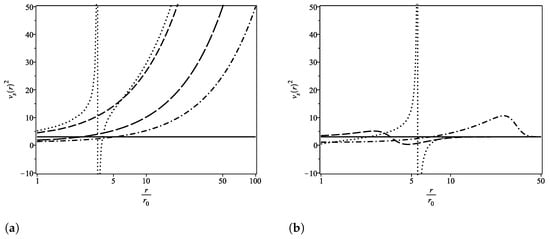

Figure 7.
Plot of versus r. In all graphs, we have (solid line), (dashdot line) and (long dashed line). In (a), we have (dashed line) and (dotted line). In (b), we have (dashed line) and (dotted line). In (c), we have (dashed line) and (dotted line). (a) global correction; (b) constant correction; (c) correction in the variable term.
3.5. Correction for Small Parameters
Although it is not possible to obtain a complete analytical solution for the redshift function in the cases considered in Section 3.1, Section 3.2 and Section 3.3, a complementary analysis is to compare the three Casimir WH generalization models for small values of the parameter . The value should model the WH for the usual Casimir case, thus small values of are on the borderline of what is already known in the literature. Furthermore, as we saw in the previous subsection, the Yukawa–Casimir WH is stable for small values of the Yukawa parameter. Therefore, the local exponential terms in can be expressed via Taylor series
so a first-order correction would be to take all terms of the type with , second-order with , and so on.
3.5.1. First Order Correction
Let us consider first-order corrections to the redshift function. In that case, we have
where and refer to cases discussed in Section 3.1, Section 3.2, and Section 3.3, respectively. Thus, the first-order corrected redshift functions of are given by
Note that, in the radial case, the solution is basically the redshift of the Casimir WH, but with a subtle change in the numerator of the logarithm argument compared to Equation (7b). This difference is due to the setting of , where additive constants have no physical implication. On the other hand, the global and constant cases behave the same way for first-order changes.
3.5.2. Second Order Correction
In first-order corrections, we observe that the redshift for the global and constant cases are the same. Furthermore, the redshift for the radial case is independent of the Yukawa parameter . In this way, it is suggestive to consider corrections in the second order. Thus,
thus, the second-order corrected redshift functions of are given by,
the behavior of these solutions as a function of is plotted in Figure 8. In this approximation order, as we see in Figure 8, the global (dashed line) and radial (dotted line) cases differ little from each other. This is why the values in these cases are close. This difference, close to the throat , becomes negligible.

Figure 8.
Behavior of the second-order modified redshift function on the parameter for Yukawa–Casimir WH.
4. Conclusions
In this work, we propose a more consistent way to generalize Casimir WH with Yukawa-type terms in shape functions in the three approaches initially proposed by Garattini [14]. Casimir WH does not have constant redshift, so there is no reason to build Yukawa–Casimir WH considering the ZTC. In our approach, we maintained the character of pressure being given by the derivative of energy, which uncovered a completely new physics for these astrophysical objects. In possession of the results obtained, the Yukawa–Casimir WH, in all considered cases, satisfies the so-called QWEC [11]
as visualized in Figure 9. In the correction in the variable term, due to the subtle discrepancies between the curves, a logarithmic scale was considered in the independent variable .

Figure 9.
Quantum Weak Energy Condition (QWEC) check. In all graphs, we have (solid line), (dashdot line), (dashed line) and (dotted line). (a) global correction; (b) constant correction; (c) correction in the variable term.
Furthermore, only in the correction of the constant term do restrictions appear on the value of the Yukawa constant since violates the flare-out condition. This type of restriction is only seen in this approach. Another characteristic of this methodology was a natural achievement, in the global and constant cases, of being possible not only to construct WH without tidal force but also to obtain cases in which the generated force is repulsive, characterizing a blueshift deviation.
Another type of restriction on the Yukawa parameter is established when studying the stability of solutions by calculating the square of the speed of sound. In this analysis, only changing the variable term did not produce unstable solutions, due to the fact that it is not very sensitive to changes in the values of . Meanwhile, for the global case, the constraint is necessary for the Yukawa–Casimir WH to be stable. Finally, in the constant case, this condition further restricted the allowed values for the Yukawa parameter, such that we must have .
In all cases, the complete solution of the redshift function cannot be obtained analytically due to local exponential terms in the integrand. Therefore, two approaches were taken. Initially, numerical integration was performed for the variable and setting , which were reproduced in Figure 2a, Figure 4a and Figure 6a. Finally, an analysis was performed for small values of the Yukawa parameter, which in the first order revealed that , while, for the radial case, the redshift function does not explicitly depend on the Yukawa parameter. On the other hand, in the second-order, it was found that the global and constant cases become slightly different. Our analysis of small parameters not only allowed us to obtain redshift analytically but also revealed insights into the boundary between the Casimir and Yukawa–Casimir wormholes. This analysis sheds light on why the value that causes the redshift to change is similar in the global (as shown in Figure 2a) and constant (as shown in Figure 4a) cases because they only differ in the second order of .
Some possible extensions of this work include dimensional generalizations, a study of the effects of the Generalized Uncertainty Principle, and analyses modifying the energy density instead of the shape function.
Author Contributions
Conceptualization, P.H.F.d.O. and G.A.; methodology, P.H.F.d.O.; validation, G.A., I.C.J. and R.R.L.; formal analysis, P.H.F.d.O. and I.C.J.; investigation, P.H.F.d.O.; writing—original draft, P.H.F.d.O.; writing—review & editing, P.H.F.d.O. and I.C.J.; supervision, G.A., I.C.J. and R.R.L. All authors have read and agreed to the published version of the manuscript.
Funding
This research was funded by Conselho Nacional de Desenvolvimento Científico e Tecnológico with grant number 315568/2021-6 and Fundação Cearense de Apoio ao Desenvolvimento Científico e Tecnológico with grant number PRONEM PNE0112- 00085.01.00/16.
Data Availability Statement
Not applicable.
Acknowledgments
The authors would like to thank the financial support provided by the Coordenação de Aperfeiçoamento de Pessoal de Nível Superior (CAPES) and by the Conselho Nacional de Desenvolvimento Científico e Tecnológico (CNPq). We also acknowledge Fundação Cearense de Apoio ao Desenvolvimento Científico e Tecnológico (FUNCAP).
Conflicts of Interest
The authors declare no conflict of interest.
References
- Schwarzschild, K. On the gravitational field of a mass point according to Einstein’s theory. arXiv 1916, arXiv:physics/9905030. [Google Scholar]
- The Event Horizon Telescope Collaboration; Akiyama, K.; Alberdi, A.; Alef, W.; Asada, K.; Azulay, R.; Baczko, A.-K.; Ball, D.; Baloković, M.; Barrett, J.; et al. First M87 Event Horizon Telescope Results. I. The Shadow of the Supermassive Black Hole. Astrophys. J. Lett. 2019, 875, L1. [Google Scholar] [CrossRef]
- Akiyama, K.; Algaba, J.C.; Alberdi, A.; Alef, W.; Anantua, R.; Asada, K.; Azulay, R.; Baczko, A.K.; Ball, D.; Baloković, M.; et al. First M87 Event Horizon Telescope Results. VIII. Magnetic Field Structure near The Event Horizon. Astrophys. J. Lett. 2021, 910, L13. [Google Scholar] [CrossRef]
- Hassan, Z.; Ghosh, S.; Sahoo, P.K.; Rao, V.S.H. GUP Corrected Casimir Wormholes in f(Q) Gravity. arXiv 2022, arXiv:2209.02704. [Google Scholar]
- Shinkai, H.A.; Hayward, S.A. Fate of the first traversible wormhole: Black hole collapse or inflationary expansion. Phys. Rev. D 2002, 66, 044005. [Google Scholar] [CrossRef]
- Maldacena, J.; Milekhin, A. Humanly traversable wormholes. Phys. Rev. D 2021, 103, 066007. [Google Scholar] [CrossRef]
- Gao, P.; Jafferis, D.L.; Wall, A.C. Traversable Wormholes via a Double Trace Deformation. J. High Energy Phys. 2017, 12, 151. [Google Scholar] [CrossRef]
- Casimir, H.B.G. On the Attraction Between Two Perfectly Conducting Plates. Indag. Math. 1948, 10, 261–263. [Google Scholar]
- Boyer, T.H. Quantum electromagnetic zero point energy of a conducting spherical shell and the Casimir model for a charged particle. Phys. Rev. 1968, 174, 1764–1774. [Google Scholar] [CrossRef]
- Avino, S.; Calloni, E.; Caprara, S.; Laurentis, M.D.; Rosa, R.D.; Girolamo, T.D.; Errico, L.; Gagliardi, G.; Grilli, M.; Mangano, V.; et al. Progress in a Vacuum Weight Search Experiment. Physics 2020, 2, 1–13. [Google Scholar] [CrossRef]
- Garattini, R. Casimir Wormholes. Eur. Phys. J. C 2019, 79, 951. [Google Scholar] [CrossRef]
- Oliveira, P.H.F.; Alencar, G.; Jardim, I.C.; Landim, R.R. Traversable Casimir wormholes in D dimensions. Mod. Phys. Lett. A 2022, 37, 2250090. [Google Scholar] [CrossRef]
- Garattini, R. Traversable Wormholes and Yukawa Potentials. arXiv 2019, arXiv:1907.03622. [Google Scholar]
- Garattini, R. Yukawa–Casimir wormholes. Eur. Phys. J. C 2021, 81, 824. [Google Scholar] [CrossRef]
- Morris, M.S.; Thorne, K.S. Wormholes in space-time and their use for interstellar travel: A tool for teaching general relativity. Am. J. Phys. 1988, 56, 395–412. [Google Scholar] [CrossRef]
- Kim, S.W. Flare-out condition of a Morris–Thorne wormhole and finiteness of pressure. J. Korean Phys. Soc. 2013, 63, 1887–1891. [Google Scholar] [CrossRef]
- Alnes, H.; Ravndal, F.; Wehus, I.K.; Olaussen, K. Electromagnetic Casimir energy with extra dimensions. Phys. Rev. D 2006, 74, 105017. [Google Scholar] [CrossRef]
- Sharif, M.; Shah, S.A.A.; Bamba, K. New Holographic Dark Energy Model in Brans-Dicke Theory. Symmetry 2018, 10, 153. [Google Scholar] [CrossRef]
Disclaimer/Publisher’s Note: The statements, opinions and data contained in all publications are solely those of the individual author(s) and contributor(s) and not of MDPI and/or the editor(s). MDPI and/or the editor(s) disclaim responsibility for any injury to people or property resulting from any ideas, methods, instructions or products referred to in the content. |
© 2023 by the authors. Licensee MDPI, Basel, Switzerland. This article is an open access article distributed under the terms and conditions of the Creative Commons Attribution (CC BY) license (https://creativecommons.org/licenses/by/4.0/).