Safety Monitor Symmetry Concerning Beam Bridge Damage Utilizing the Instantaneous Amplitude Square Method

Abstract

It is critical for the safety monitoring of highway bridges that beam bridge damage can be identified from the dynamic response of passing vehicles. Numerical simulations of passing vehicles were conducted utilizing the vehicle–bridge coupling vibration theory and the indirect measurement method. Fast Fourier transform was performed on the time history response of vehicle acceleration, and the driving frequency component response and its instantaneous amplitude square value (IAS value) were obtained by band-pass filtering and Hilbert transform processing. The identified IAS value detected the damage location of the bridge. The identification method of IAS value is used to analyze the applicability of a simply supported beam bridge, a continuous beam bridge, and an irregular skew beam bridge. The effects of vehicle speed, vehicle damping, bridge damping, and a social vehicle on damage identification are discussed. The results show that the effect of damage location is better when the vehicle speed is less than 4 m/s. In the presence of social vehicles, the excitation on the bridge increases, and the damage location can still be accurately determined by the IAS method. Vehicle damping and bridge damping have little effect on the results of damage identification. In structural health monitoring for bridges, this paper can provide a theoretical reference for the application of IAS motion sensing to identify the damage location indirectly.

1. Introduction

With increases in the service life of bridges, more and more bridges have been damaged to varying degrees. In order to ensure the safety of the structure and the operation of the bridge, it is very important to monitor or detect the health of the bridge. The early detection of damage to a bridge and emergency repair can effectively improve the service life of the bridge [1,2,3,4,5]. In order to obtain the modal characteristics of a bridge, the direct measurement method is widely used, but this method needs sensors installed on the bridge, which not only interrupts traffic but is also time-consuming and laborious.

Yang et al. [6] first proposed the “indirect measurement method” based on a vehicle’s response to identify the dynamic characteristics of bridges in 2004. Subsequently, Lin et al. [7] verified the effectiveness of the method through field tests in 2005, and scholars from various places have successively carried out related studies. The basic idea is that after the vehicle passes the bridge, at each point of the bridge, the vertical vibration of the vehicle causes the vertical vibration of the bridge. Due to the coupling between the vehicle and the bridge, the vertical vibration of the bridge reacts to the vehicle and acts as the main vehicle. The vertical excitation source, through the relevant signal processing of the vertical vibration acceleration of the vehicle, further obtains the relevant dynamic characteristic information of the bridge. Since the method was proposed, it has received extensive attention from many scholars at home and abroad, and a series of innovative research results has been achieved and is expected to provide new ideas for the rapid testing and safety diagnosis of the health status of small- and medium-span bridges [8,9,10].

Since the “indirect measurement method” came out more than 10 years ago, scholars from all over the world have applied it to the field of bridge modal parameter identification and bridge health monitoring. The corresponding research has mainly gone through the following stages: the indirect measurement method is proposed; identification of bridge frequency; identification of bridge mode; identification of bridge damping; identification of bridge damage. The modal shape of a bridge, which has been extensively investigated by scholars, is an essential parameter that reflects the structural characteristics of the bridge. Using the indirect measurement method to identify the analytical solution formula of bridge frequency through band-pass filtering, Hilbert–Huang transform, and other signal processing techniques, Yang et al. [11,12] identified the mode shape of a simply supported girder bridge from the vertical acceleration time history response of vehicles, derived an analytical solution to identify the mode shape of the bridge, and roughly discussed the influence of bridge deck unevenness, traffic flow, and vehicle speed on the first-order vibration shape of the bridge. Yang et al. [13] used the vertical acceleration signals collected by two stationary vehicles on a bridge to calculate the vertical displacement of the contact point between the vehicle and the bridge, then changed the position of the vehicle, collected signals repeatedly, and constructed a matrix combined with the SVD method to extract the mode shape of the bridge. Qi et al. [14] proposed a method of impacting the vehicle body to identify the mode shape of a three-span continuous girder bridge by increasing the excitation of the bridge and overcoming the interference of white noise and bridge deck unevenness on mode shape identification and identified the first three modes of the continuous girder bridge. In addition, the short-time frequency decomposition technology proposed by scholars has improved the accuracy of the modal shape identification of bridges [15,16]. In addition, the combination of band-pass filtering and hanning window technology has solved the limitation of the low-speed driving of vehicles [17], and the tractor trailer system combines the short-time Fourier transform (STFT) method to eliminate the interference caused by vehicle frequency and road roughness [18,19,20,21]. Yang et al. [9] summarized the indirect measurement method, clarifying the convenience of the indirect measurement method in practical engineering applications and the insufficiency of research, especially in the limitations of vehicle models.

Bridge damage location is the ultimate goal of the research. Based on the vehicle–bridge interaction, the researchers used the reconstructed first-order bridge mode shape, combined with the curvature mode method [22] and the improved direct stiffness method [23,24,25], to determine the damage location of the bridge. In addition, using the signals collected by the measuring vehicle, combined with the element stiffness index (ESI) [26], empirical mode decomposition (EMD) [27], genetic algorithm (GA) [28], wavelet transform [29], bridge displacement profile difference [30,31], global filtering method (GFM) [32], instantaneous curvature (IC) [33], vehicle transmissibility [18], wavelength characteristics [34], approximate Metropolis–Hastings (AMH) algorithm and the probability density evolution method [35], instantaneous amplitude square (IAS) [36,37,38], and other indicators and techniques have achieved fruitful results in the field of bridge damage identification.

Bridge damage identification based on vehicle response does not require on-site installation of detection instruments and has the advantages of high efficiency, convenient operation, and cost savings. In view of the superiority of the IAS method in [38], this paper further expands the application scope of the IAS method in different structural forms of girder bridges; this paper takes the simply supported beam bridge, continuous beam bridge, and skew beam bridge as the research objects and accurately locates the damage location of the beam bridge through numerical simulation. The parameters, such as vehicle speed, social vehicle, damage degree, vehicle damping, and bridge damping, are analyzed in detail, which provides a reference for the application of the IAS method in practical engineering.

2. Indirect Measurement Theory

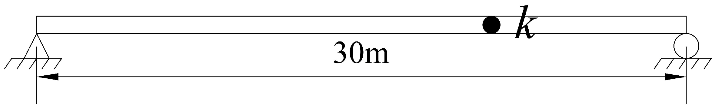
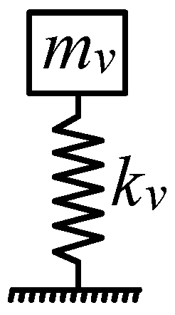
As shown in Figure 1, a single-degree-of-freedom vehicle is used to pass a simply supported beam bridge, and the theoretical solution of the vehicle is derived based on this model. It is worth noting that this theory is also applicable to other beam bridge forms.

The single-axle 1/4 vehicle is modeled into a sprung mass with a mass of $m_v$, and the spring stiffness is $k_v$. The mass per unit length of the bridge is taken as $\overline{m}$, the bending stiffness of the section is EI, and the deflection at the coordinate x of the bridge is $u(x)$; the derivation process of the formula is referred to in [37].

Discretize the bridge, and the equation of motion of the bridge is listed as follows:

$$\overline{m}\ddot{u}(x,t)+EI{u}^{″″}(x,t)=f_c(t)\delta (x-vt)$$

(1)

The equation of motion of the vehicle is listed as follows:

$$m_v{\ddot{q}}_v(t)+k_v(q_v(t)-u(x,t){|}_{x=vt})=0$$

(2)

Omitting the intermediate process of formula derivation, the acceleration response of the vehicle is:

$${\ddot{q}}_v(t)={\displaystyle \sum _{n=1}^{\infty }\frac{{\Delta }_{st,n}}{2(1-S_n^2)}}\left[{\overline{\overline{A}}}_{1n}\cos ({\omega }_{v}t)+{\overline{\overline{A}}}_{2n}\cos (\frac{2\pi nvt}{L})+{\overline{\overline{A}}}_{3n}\cos ({\omega }_{b,n}t-\frac{n\pi vt}{L})+{\overline{\overline{A}}}_{4n}\cos ({\omega }_{b,n}t+\frac{n\pi vt}{L})\right]$$

(3)

where

$${\overline{\overline{A}}}_{1n}={\omega }_v^2\left[\frac{-{\omega }_v^2}{{\omega }_v^2-{(\frac{2n\pi v}{L})}^2}+\frac{-{\omega }_v^2{S}_n}{{\omega }_v^2-{({\omega }_{b,n}-\frac{n\pi v}{L})}^2}+\frac{{\omega }_v^2{S}_n}{{\omega }_v^2-{({\omega }_{b,n}+\frac{n\pi v}{L})}^2}+1\right]$$

$${\overline{\overline{A}}}_{2n}=\frac{{\omega }_v^2{(\frac{2\pi nv}{L})}^2}{{\omega }_v^2-{(\frac{2n\pi v}{L})}^2},{\overline{\overline{A}}}_{3n}=\frac{{\omega }_v^2{S}_n{({\omega }_{b,n}-\frac{n\pi v}{L})}^2}{{\omega }_v^2-{({\omega }_{b,n}-\frac{n\pi v}{L})}^2},{\overline{\overline{A}}}_{4n}=\frac{-{\omega }_v^2{S}_n{({\omega }_{b,n}+\frac{n\pi v}{L})}^2}{{\omega }_v^2-{({\omega }_{b,n}+\frac{n\pi v}{L})}^2}$$

$${\Delta }_{st,n}=\frac{-2m_{v}g{L}^3}{n^4{\pi }^{4}EI},S_n=\frac{n\pi v}{L{\omega }_{b,n}}$$

(4)

where ${\omega }_{b,n}$ is the nth-order natural frequency of the bridge; ${\omega }_v$ is the vertical vibration frequency of the vehicle; ${\Delta }_{st,n}$ is the static displacement of the nth-order mode of the bridge under the action of the vehicle, and $S_n$ is the dimensionless velocity parameter; L is the total length of the bridge; v is the moving speed of the vehicle; $m_v$ is the mass of the moving vehicle; EI is the bending stiffness of the bridge.

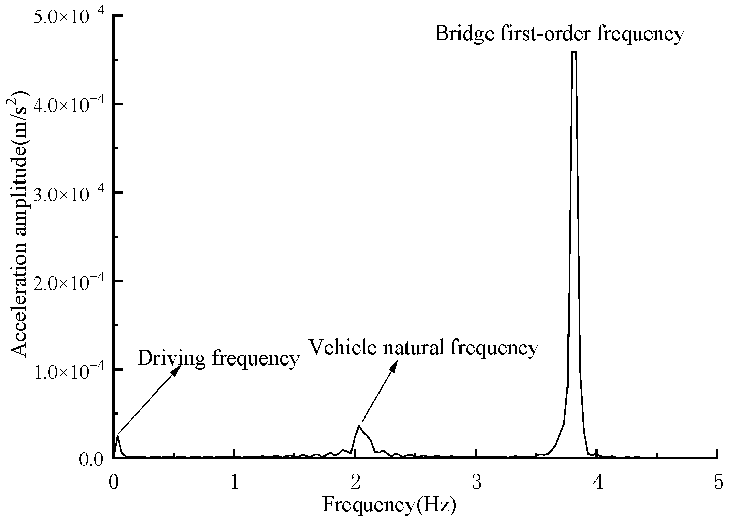
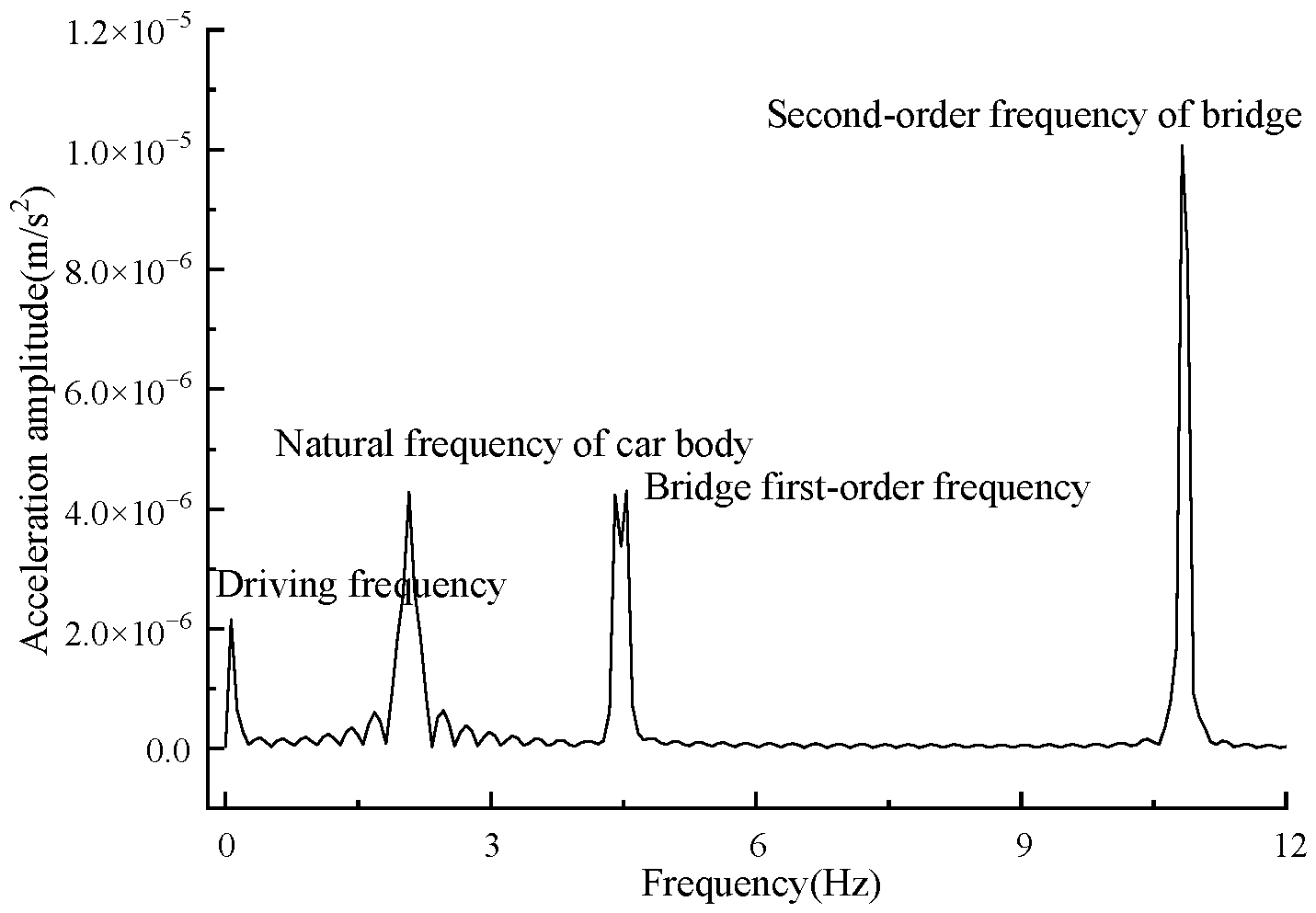
The analytical solution of the vehicle acceleration time history response is composed of three different types of frequency superposition, which are the natural frequency of the vehicle ${\omega }_v$, the driving frequency $2n\pi v/L$, the left-shift frequency ${\omega }_{b,n}-n\pi v/L$, and the right-shift frequency of the bridge ${\omega }_{b,n}+n\pi v/L$.

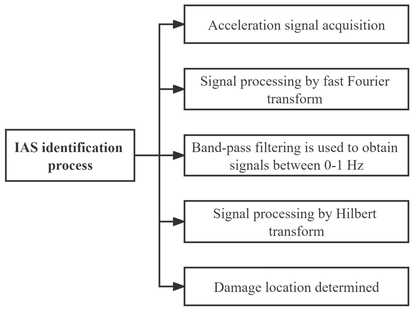
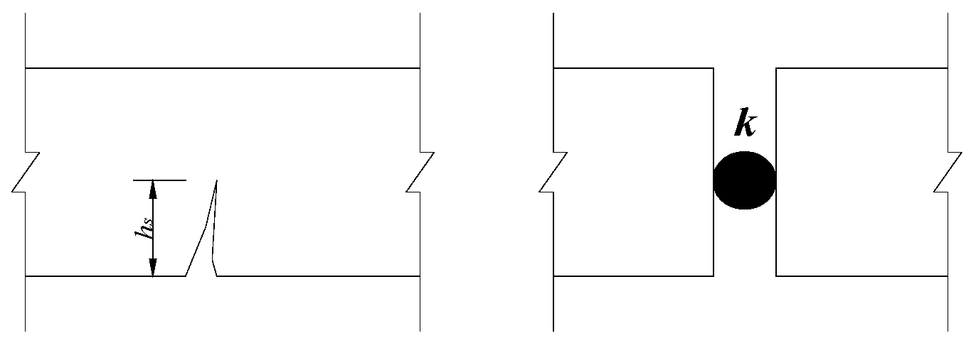
The IAS method is a new bridge damage location identification method based on Hilbert transform. The IAS value is defined as follows:

$$A^2\left[R_d(x)\right]={\displaystyle \sum _{n=1}^M{A}_n^2}+2{\displaystyle \sum _{n=1}^M{\displaystyle \sum _{k=2}^M{A}_n{A}_k\left[1-2{\varphi }_{k-n}^2(x)\right]}}$$

(5)

R_d(x) is the driving component response of vehicle acceleration, where ${\varphi }_n(x)=\sin \frac{n\pi x}{L}$, ${\varphi }_n(x)$ is a modal function; when the bridge is damaged, the modal function has a sudden change.

3. Numerical Analysis

3.1. IAS Identification Process

Based on the principle of separation method and vehicle dynamics theory, the vehicle model and the bridge model are modeled separately, and the constraint equation is used to realize the coordinated relationship between the displacement of the wheel and the bridge surface contact point at any time (the corresponding force balance relationship is automatically satisfied). APDL programming is used to conduct the coupled dynamic time history response analysis of vehicles crossing the bridge [39,40,41].

Generally, there are four main types of bridge damage models: the stiffness drop model, the open crack model, the breathing crack model, and the torsion spring model. The stiffness reduction model is a relatively common bridge damage model. When performing damage simulation, it mainly reduces the bending stiffness of the damaged part of the bridge. The advantage is that it is easy to define in finite element software. The disadvantage is that it does not take into account the impact on the adjacent parts; the open crack model mainly simulates the condition of open cracks. The basic simulation principle is the failure of the flexural rigidity of a certain part of the lower part of the open crack. Breathing cracks mainly consider the opening and closing effects of cracks under load; the torsion spring model mainly considers the connection between two nodes, and the part between the two nodes is simulated as a linear spring, which mainly considers the displacement and rotation angle of the two nodes [42,43].

The damage model of the beam bridge is simulated with an open crack model. The finite element simulation method is to insert a rotating spring with zero length between two adjacent beam elements. When a crack occurs at a certain position of the beam, the left and right sides of the crack will not be misaligned and only the attenuation of the rotational stiffness occurs.

The stiffness matrix of the crack element is as follows [44]:

$$K_l=\left[\begin{array}{c}\begin{array}{cc}K& -K\end{array}\\ \begin{array}{cc}-K& K\end{array}\end{array}\right]$$

(6)

whose element is defined as follows [44]:

$$K=\frac{EI}{2h{\left(\frac{\beta }{1-\beta }\right)}^2\left(5.93-19.69\beta +37.14{\beta }^2-35.84{\beta }^3+13.12{\beta }^4\right)}$$

(7)

where the damage factor β is defined as the ratio of the beam damage height to the beam height.

The IAS identification process is shown in Figure 2; the specific damage identification steps are as follows:

(1) Obtain the vertical acceleration time history response of the vehicle body when driving over the bridge;

(2) Obtain car body acceleration response spectrogram through fast Fourier transform;

(3) Determine the narrowband range of the acceleration response time history corresponding to the driving frequency and intercept the acceleration time response of the driving frequency part through band-pass filtering;

(4) Take the Hilbert transform of the acceleration time history signal obtained by band-pass filtering and square the result;

(5) Identify the damage location of the bridge by the peak value.

3.2. Applicability Analysis of Different Beam Bridge Forms

In order to discuss the applicability of the IAS method, this section selects three types of girder bridges for discussion, namely, simply supported girder bridges, continuous girder bridges, and oblique girder bridges. In order to improve the accuracy of recognition, the vehicle speed is 1 m/s. When establishing the ANSYS finite element crack damage model, the rotating spring is simulated by the combin7 element. The two nodes of this element overlap, which can define the translational stiffness and rotational stiffness of adjacent nodes and can better simulate the cracks of the beam. The schematic diagram of the crack model is as follows, as shown in Figure 3.

3.2.1. Simply Supported Girder Bridge

We assume that the total length of the bridge L is 30 m, the unit mass density ρ is 1000 kg/m, Young’s modulus E is 27.5 GPa, the inertial moment I is 0.175 m⁴, the mass of the mobile measuring vehicle m_v is 1000 kg, the stiffness k_v is 170 kN/m, the natural vibration frequency of the vehicle ${\omega }_v$ is 2.08 Hz, and the moving speed v is 1 m/s. A schematic diagram of a simply supported beam bridge is shown in Figure 4; the modal information of the simply supported beams is shown in

Table 1. Bridge natural vibration frequency and mode characteristics (simply supported girder bridge).

Order	Frequency (Hz)	Cycle (s)	Mode Characteristics
1	3.82	0.26	Main beam symmetrical vertical bending
2	15.26	0.07	Main beam anti-symmetric vertical bending
3	34.17	0.03	Main beam symmetrical vertical bending

. The impact of bridge and vehicle damping is not considered for the time being. The time step Δt is 0.01 s. In the finite element method, the bridge is divided into 3000 units, and the length of each unit is 0.01 m.

(1)

Damage identification of a single vehicle

A crack with a damage coefficient β of 0.2 is applied at a distance of 21 m from the left end of the beam, and the vehicle speed is 1 m/s. A numerical simulation test was performed on it. The vehicle acceleration time history is shown in Figure 5.

The frequency spectrum of the vehicle acceleration time-course information is transformed, and the driving frequency value is 0.033 Hz; the vehicle body frequency spectrum is shown in Figure 6.

According to the vehicle spectrogram, band-pass filtering technology is used to filter out the 0–1 Hz of the vehicle acceleration time history information, and the acceleration time history signal of the driving frequency signal is obtained, as shown in Figure 7. It should be noted that the filtering range used in this paper is not unique. When the vehicle speed is 1 m/s, since the first-order driving frequency is very small, the range of 0–1 Hz includes the first 30-order driving frequency. Theoretically, the more high-order driving frequencies are included, the more accurate the recognition results are. However, due to the limitation of vehicle frequency and bridge frequency, the filtering range has an upper limit. Studies have shown that more accurate damage location information can be obtained by extracting the first ten driving frequencies [45]. In the process of damage location, in order to avoid the interference of vehicle frequency leakage, the stiffness of the measuring vehicle should be improved as much as possible.

Hilbert transform is performed on the obtained driving frequency component response, and the instantaneous amplitude of the driving frequency component response is obtained. The instantaneous amplitude is squared, and the IAS value is shown in Figure 8.

It can be seen from Figure 8 that when the damage is identified based on the vehicle response, there will be a large number of fluctuations with small magnitudes, which corresponds to the free vibration of the vehicle. Twenty percent crack damage was applied at a distance of 21 m from the left end. The location of the crack damage can be clearly identified in Figure 8, and the peak value is more prominent. The IAS method has a good identification effect for the crack damage of common simply supported beam bridges.

(2)

The impact of social vehicles on damage recognition

The bridge model adopts the simply supported beam model introduced in Section 3.2.1. A crack with a damage coefficient β of 0.2 is applied at 21 m from the left end point of the beam; the vehicle runs at a constant speed of 1 m/s. In order to simulate the traffic situation of the bridge, two vehicles with the same characteristics are added to the rear of the measuring vehicle (these are called social vehicles in this paper), and the distance between the three vehicles is a constant distance of 1 m, the IAS value is shown in Figure 9.

As can be seen from Figure 9, when identifying damage based on the vehicle response, there is a large number of small peaks, which correspond to the free vibration of the vehicle. When the car is going up and down the bridge, at this time, due to the sudden change of the parameters of the axle response system, there are bumps at the head and tail of the bridge. Twenty percent crack damage was applied at a distance of 21 m from the left end. The position of the crack damage can be clearly identified in Figure 9, and the peak value is more prominent. The IAS method has a relatively accurate identification effect on the crack damage of common simply supported beam bridges. When there are other vehicles on the bridge, it is equivalent to increasing the excitation effect on the bridge, and the slight damage of the bridge can still be reflected in the vertical vibration of the test vehicle, which is beneficial to bridge damage identification, and the bridge damage can still be identified.

3.2.2. Continuous Beam Bridge

A numerical simulation test of a 28 + 45 + 28 m three-span continuous girder bridge is carried out. The bridge is a single-box single-chamber main girder with a bridge deck width of 8 m. The main girder of the whole bridge employs C50 prestressed concrete, and the elastic modulus E_C is 3.45 × 10⁴ MPa. The middle beam and end beam of the bridge are simulated as rigid bodies.

The basic parameters of the bridge are shown in

Table 2. Longeron parameters of bridges.

Span Combination (m)	Mass per Unit Length (kg·m−1)	Moment of Inertia of Section (m4)	Sectional Area (m2)	Elastic Modulus (GPa)
28+45+28	10,963	2.5	9.87	3.45

; the modal parameters of the continuous beam bridge are shown in

Table 3. Bridge natural vibration frequency and mode characteristics (continuous beam bridge).

Order	Frequency (Hz)	Cycle (s)	Mode Characteristics
1	3.11	0.32	Main beam symmetrical vertical bending
2	6.36	0.16	Main beam anti-symmetric vertical bending
3	7.44	0.13	Main beam symmetrical vertical bending

.

The vehicle adopts a 1/4 single-degree-of-freedom vehicle model, allowing it to drive across the bridge at a constant speed. The vehicle finite element modeling is shown in Figure 10.

The vertical vibration frequency calculation formula is shown in Equation (8).

$${\omega }_v=\frac{1}{2\pi }\sqrt{\frac{k}{m}}$$

(8)

The damage location is 58 m away from the left end of the bridge, as shown in Figure 11; the damage coefficient is 0.2.

The vertical acceleration time history response of the vehicle driving over the three-span continuous beam bridge is extracted, and the result is shown in Figure 12.

It can be seen from Figure 12 that when the car body passes through the bridge crack position, the acceleration value has a slight sudden change. This is because the vehicle vibration is completely generated by the excitation of the bridge, and any slight change in the internal structure of the bridge will affect the acceleration response of the vehicle. Here, the vehicle does not consider the impact of its own damping.

Fast Fourier transform is performed on the vehicle body’s vertical acceleration time history response, and the vehicle body response spectrum is shown in Figure 13.

Band-pass filtering is performed on the obtained vehicle vertical acceleration time history response to obtain the component response of the driving frequency. According to the frequency spectrum (Figure 13), take the filter band of 0–1 Hz. The driving frequency component response is shown in Figure 14.

Hilbert transform is performed on the driving frequency component response, and the obtained instantaneous amplitude is squared to obtain the IAS value. The IAS value identification diagram is shown in Figure 15.

The identification value is 58.4 m, and the error value is 0.69%, indicating that the IAS method can better identify the crack damage location of continuous beam bridges.

3.2.3. Oblique Beam Bridge

The engineering example is a concrete simply supported slab bridge with a span of 15.41 m; the oblique angle is $30°$, the bridge deck width is 4.9 m, and the beam height is 0.8 m. The main girder of the whole bridge is made of C40 reinforced concrete, and the elastic modulus E_C is 3.25 × 10⁴ MPa. The relevant structural parameters of the main girder of the bridge are shown in

Table 4. Structure parameters of the main girder of the bridge.

Span (m)	Mass per Unit Length (kg·m−1)	Moment of Inertia of Section (m4)	Sectional Area (m2)	Elastic Modulus (GPa)
15.41	10,192	0.657	3.92	32.5

.

There are five plate rubber bearings at both ends of the plate beam, and the distance between adjacent supports is 1 m. When building the bridge model in finite elements, the span of the inclined end beam is 1 m in length; the relevant structural parameters of the end beam are shown in

Table 5. Structural parameters of the end beam.

Span (m)	Mass per Unit Length (kg·m−1)	Moment of Inertia of Section (m4)	Sectional Area (m2)	Elastic Modulus (GPa)
1	416	0.019	0.16	32.5

. The beam4 element is used to establish the calculation model of the skew bridge.

The modal analysis of the bridge model is carried out, and the natural frequency and mode characteristics of the bridge are shown in

Table 6. Bridge natural vibration frequency and mode characteristics (oblique beam bridge).

Order	Frequency (Hz)	Cycle (s)	Mode Characteristics
1	4.50	0.22	Main beam anti-symmetric vertical bending, diagonal cross beam anti-symmetric vertical bending
2	11.29	0.09	Symmetrical vertical bending of main beam, twisting of diagonal cross beam
3	38.88	0.03	Main beam anti-symmetric vertical bending, diagonal cross beam torsion

.

Crack damage with a damage coefficient of 20% is applied at 11.6 m from the left end of the bridge. A single-axle 1/4 vehicle model is used to drive across the skew slab bridge at a constant speed of 1 m/s, and the vehicle acceleration time history response is obtained, as shown in Figure 16.

Figure 17 shows that the first-order frequency peak of the bridge is relatively low, which is the combined vibration of the bridge main girder and the oblique end crossbeam, both showing the form of anti-symmetric vertical bending vibration. The second-order frequency peak of the bridge is the highest because the bridge’s main girder presents symmetrical vertical bending and has the largest contribution to vehicle vibration; the driving frequency component response is shown in Figure 18. From the IAS value identification in Figure 19, it can be concluded that the damage identification position is 11.96 m and the identification error is 3.10%, which meets the engineering accuracy requirements. Numerical simulation experiments show that the method of identifying the location of bridge crack damage based on the IAS value is also applicable to irregular oblique girder bridges.

4. Effect of Vehicle Speed on IAS Value

The damage identification of the three-span continuous beam bridge in Section 3.2.2 is based on the IAS method. In different numerical tests, the vehicle adopts a 1/4 single-degree-of-freedom vehicle model and analyzes the case of continuous beam driving at a constant speed at five different speeds. According to the basic principle of an indirect measurement method, vehicle speed has the same law of action on different beam bridge forms, so this section only selects a continuous beam bridge for vehicle speed discussion.

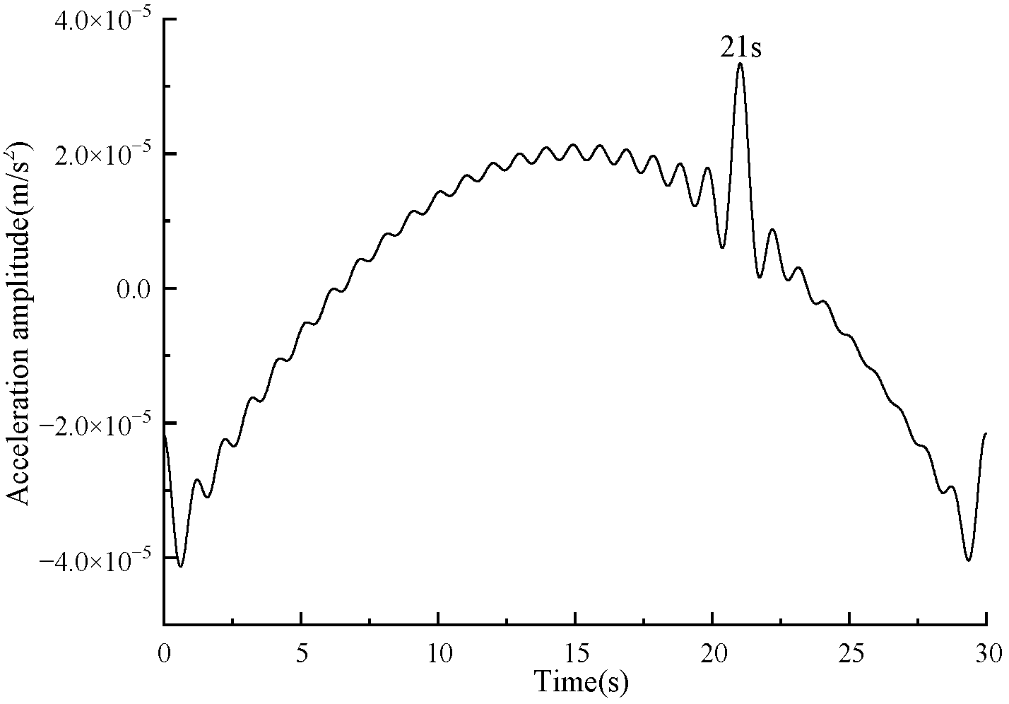
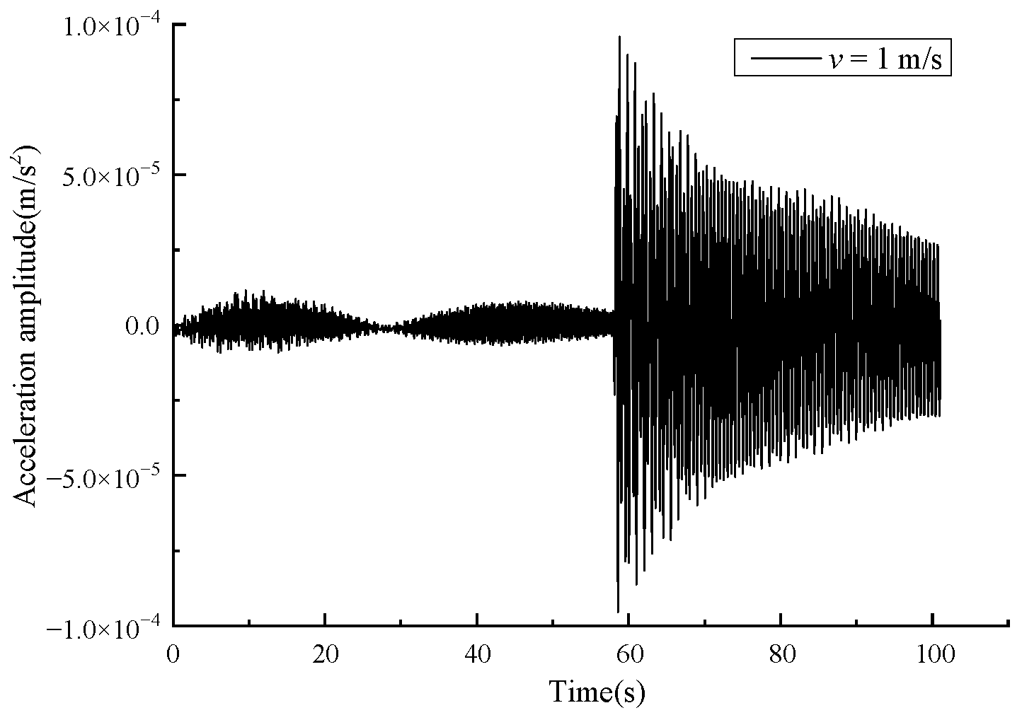
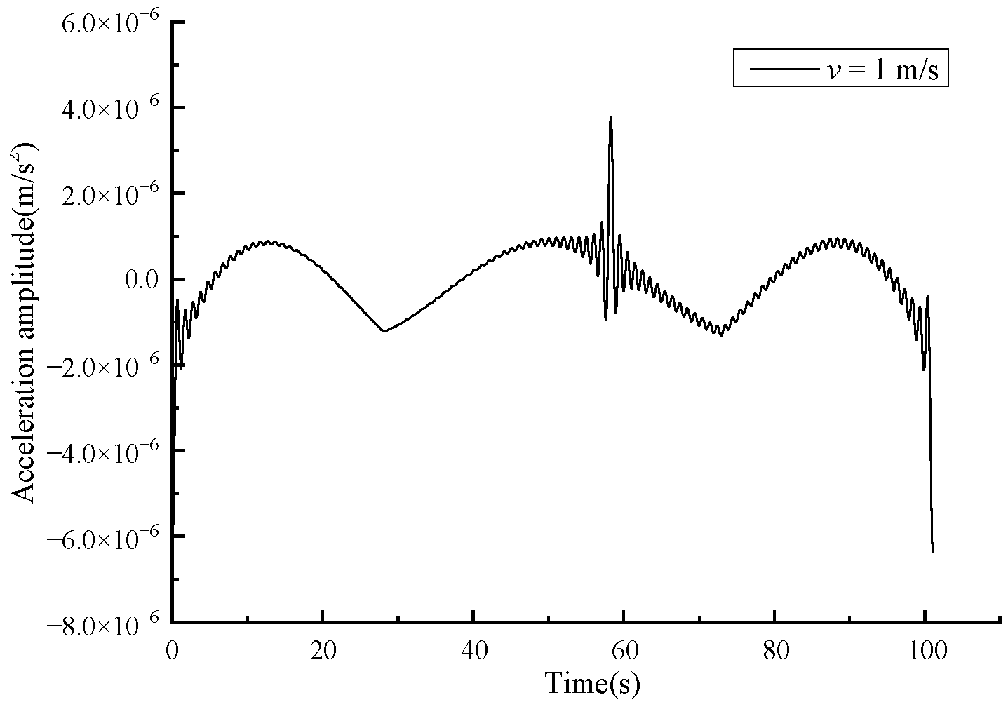
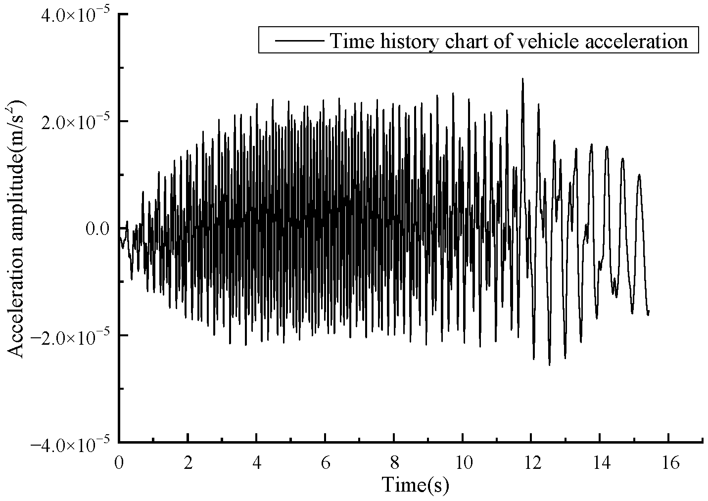
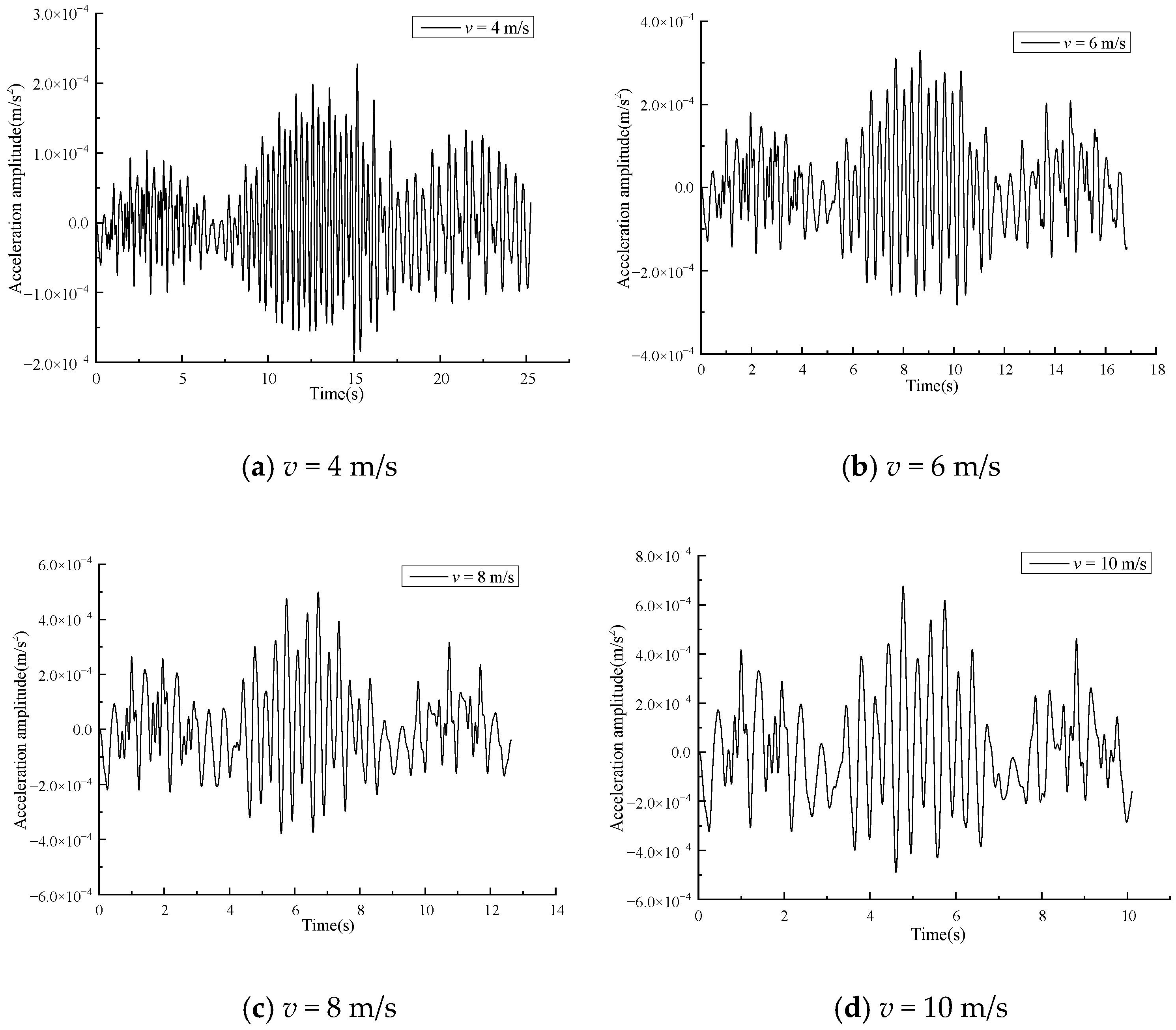
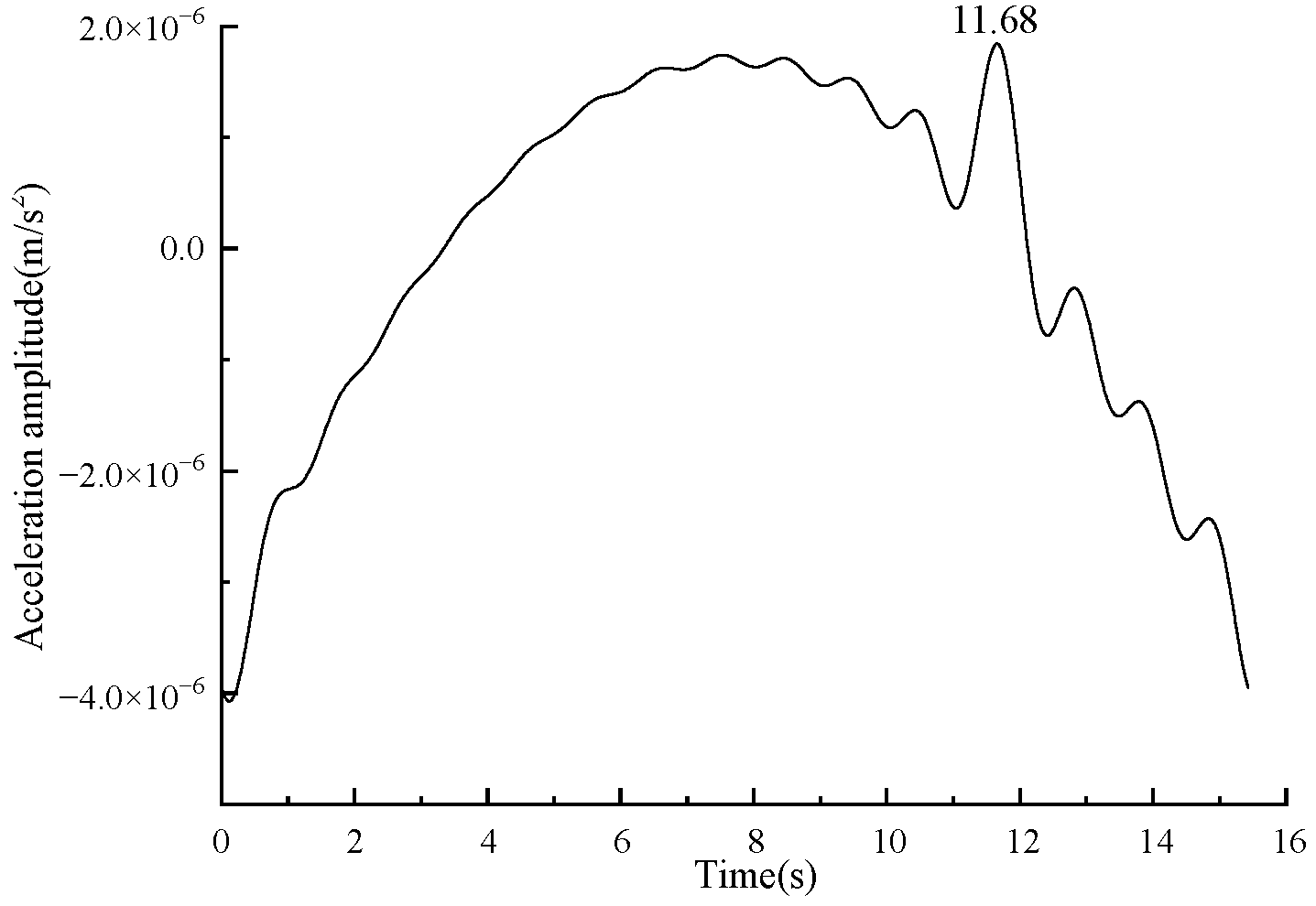
The vertical acceleration time history response of the vehicle driving through the three-span continuous beam bridge is extracted, and the result is shown in Figure 20, when the vehicle speed is 1m/s, the time history diagram of vehicle acceleration is shown in Figure 16.

It can be seen from Figure 16 and Figure 20 that when the vehicle passes through the bridge crack position, the acceleration value has a slight sudden change. This is because the vehicle vibration is completely generated by the excitation of the bridge, and any slight change in the internal structure of the bridge will have an impact on the acceleration response of the vehicle. Here, the vehicle does not consider the impact of its own damping. As the vehicle speed increases, it can be seen that the sudden change in amplitude at the crack location is gradually insignificant or even difficult to identify. This is because the higher the vehicle speed, the weaker the vehicle’s ability to collect bridge information, especially the microscopic damage. In addition, the filtering range used in this paper is 0–1 Hz. When the vehicle speed increases, the first-order driving frequency increases, the high-order driving frequency in this filtering range decreases, and the damage information contained in the IAS identification diagram lessens. 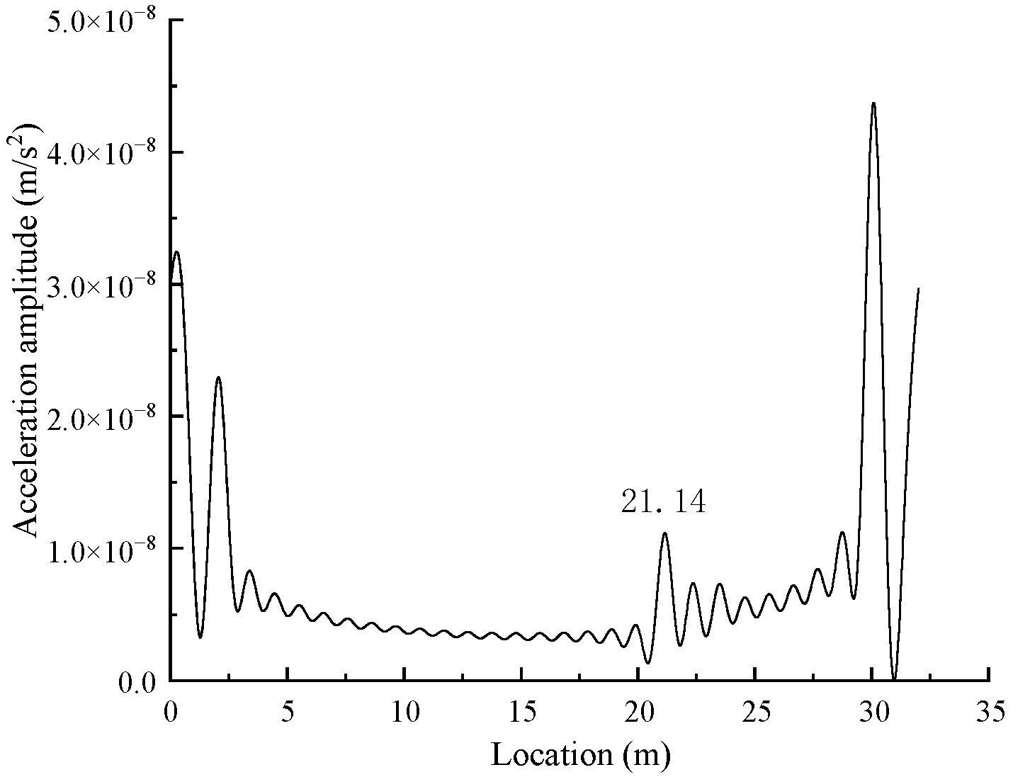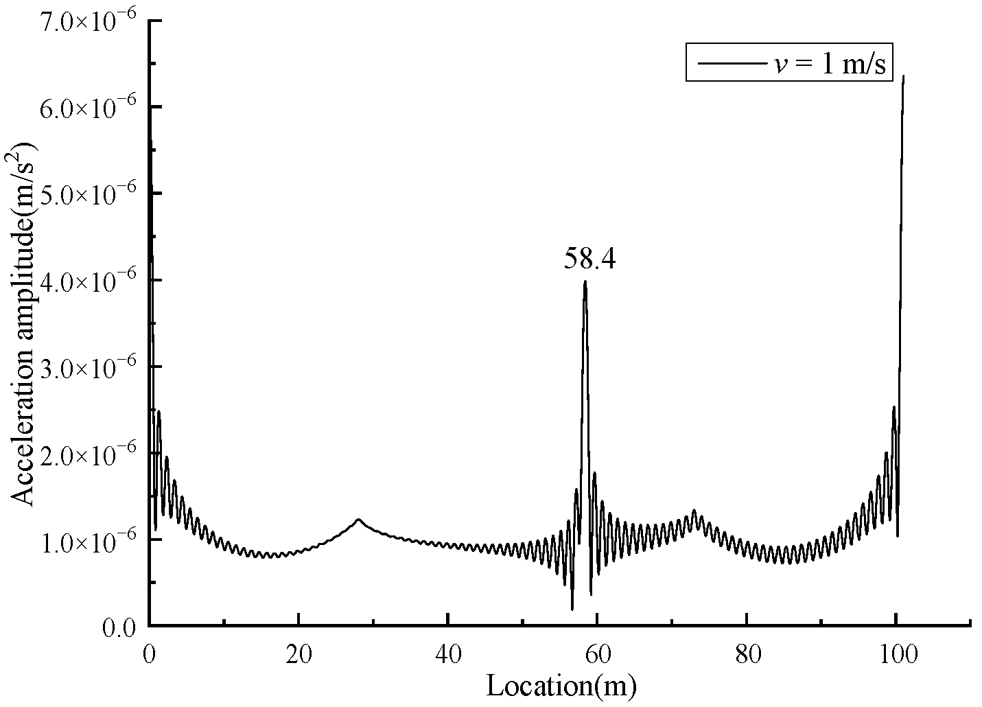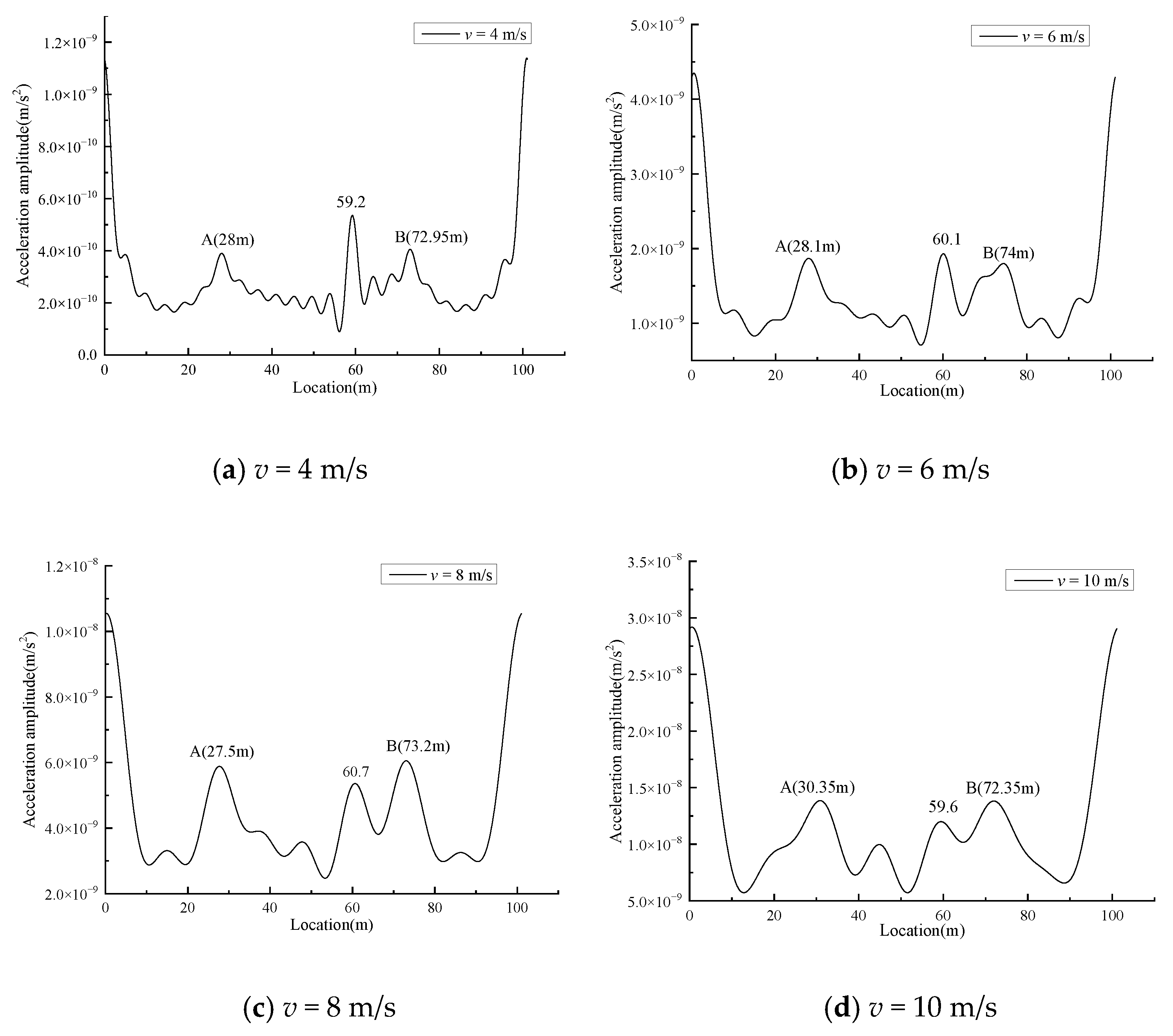As the filtering range is not unique, the filtering range can be appropriately expanded in the identification process, and attention should be paid to avoiding the interference of the vehicle’s own frequency signal leakage [45]. In the process of vehicle design, in order to reduce the influence of vehicle frequency, the stiffness of the vehicle should be increased as much as possible. 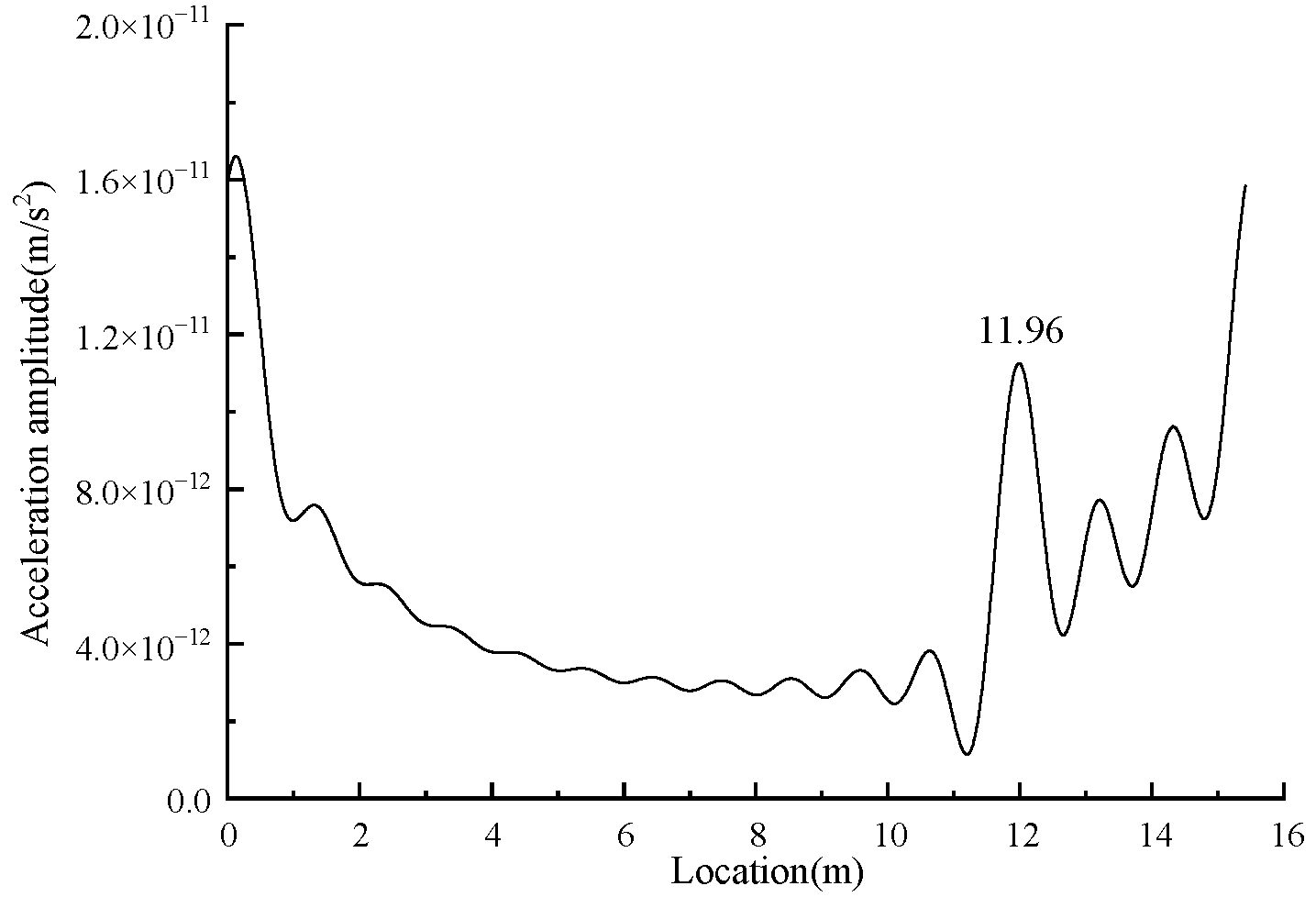IAS identification results are shown in Figure 21, When the speed is 1m/s, IAS recognition results are shown in Figure 15. The relationship between bridge damage identification accuracy and vehicle speed is shown in Figure 22 and

Table 7. Identification error value of the IAS value.

Speed (m/s)	1	4	6	8
Identification value (m)	58.4	59.2	60.1	60.7
Difference (%)	0.69	2.06	3.62	4.66

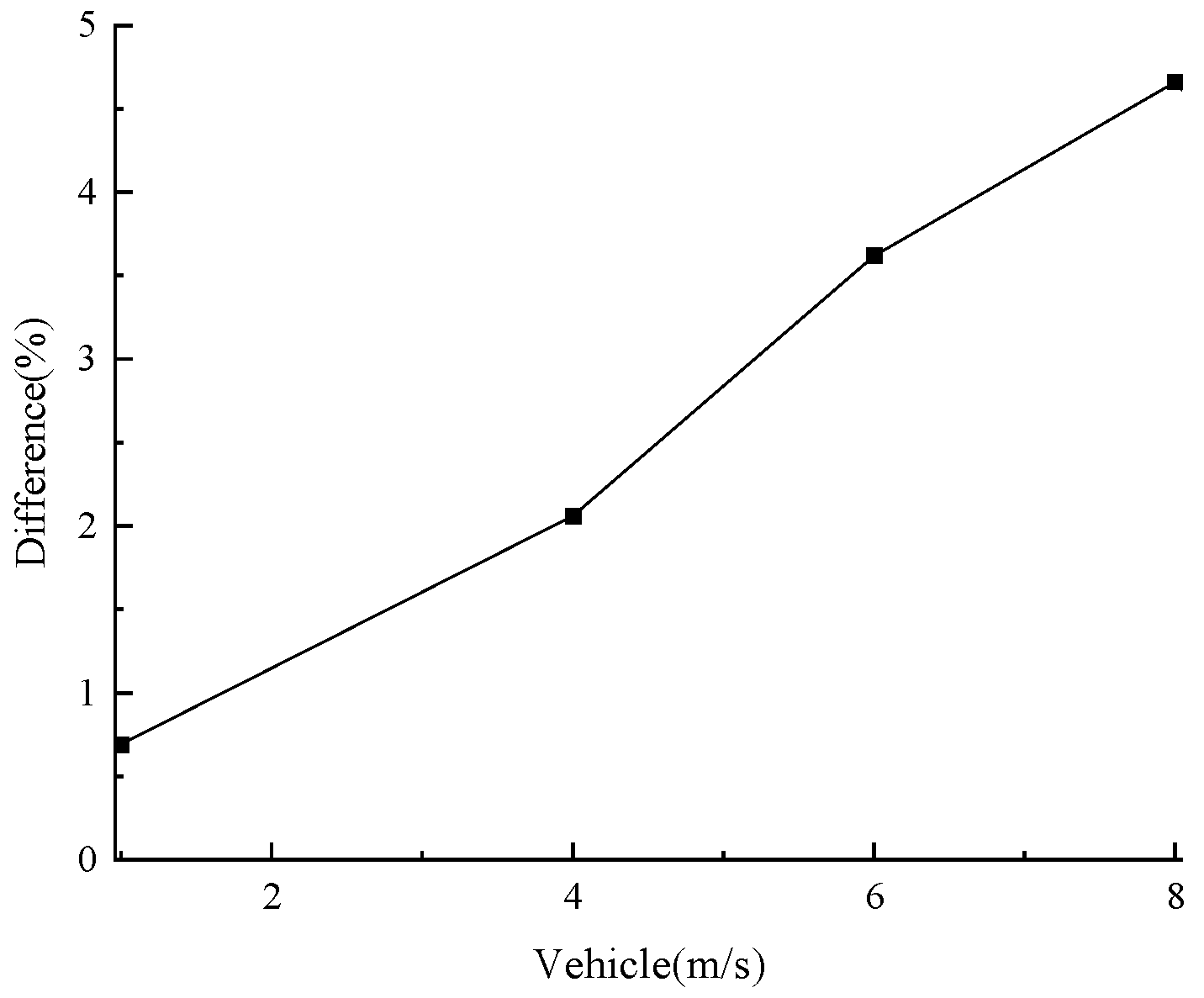
. It can be seen from Figure 15 and Figure 21 that with the increase in vehicle speed, the peak resolution of the damage position in the IAS diagram decreases. Since the IAS method can accurately detect the change in the stiffness of the bridge structure, protrusions will occur at the bridge bearing position, corresponding to points A and B. When the vehicle speed is 4 m/s and below, the IAS method can preferably identify the crack damage location of the bridge. When the vehicle speed is between 4–8 m/s, it is prone to damage misjudgment. At this time, the damage location can be determined by artificially eliminating the protrusions at the bearing position. When the vehicle speed is 10 m/s, the damage location cannot be determined. It can be seen from Figure 22 that as the vehicle speed increases, the damage location identification error increases. In actual bridge detection, it is recommended that the measuring vehicle travels at a uniform speed of no more than 4 m/s.

5. Effect of Damage Degree on IAS Value

This section sets $\alpha$ = 0.05, 0.1, 0.2 for three different degrees of bridge damage; vehicle and bridge characteristics remain the same as in Section 3.2.1. The IAS identification results are shown in Figure 23. From Figure 23, it can be seen that the acceleration amplitude at the damage increases with the increase of the damage degree. When the damage degree is $\alpha \ge 0.1$, the location of the damage can be identified quickly and accurately; when the damage degree is $0.01\le \alpha \le 0.05$, the protrusion at the damage site is smaller and the accuracy is reduced; however, the IAS identification map can still be used for the preliminary positioning of the bridge damage location.

6. Effect of Damping on IAS Value

6.1. Vehicle Damping

In the previous calculation, the damping of the vehicle is not considered, but in the actual measurement vehicle manufacturing process, the damping of the vehicle is inevitable. In the calculation process, the damping of the bridge is assumed to be Rayleigh damping, damping ratio $\xi$ = 0.02, and the other parameters of the bridge are the same as in Section 3.2.1. Using ${\xi }_v$ = 0, 0.02, 0.05, 0.1, four degrees of the vehicle damping ratio, the IAS identification results are shown in Figure 24. It can be seen from Figure 24 that the change in the vehicle damping ratio has no effect on the IAS identification results. This is because vehicle damping primarily affects the high-frequency component of the vehicle’s response and not the driving frequency component used for the IAS value calculation [37]. The IAS method can still accurately locate the damage even if vehicle damping exists.

6.2. Bridge Damping

This section uses the vehicle damping ratio ${\xi }_v$ = 0.1 to calculate four different bridge damping ratios, considering $\xi$ = 0, 0.02, 0.03, 0.05; the IAS identification results are shown in Figure 25. It can be seen from Figure 25 that when the bridge damping ratio is different, the IAS results have slight changes at the starting and ending points of the bridge, while the IAS results are almost the same at other positions on the bridge. There are obvious protrusions at the damage position, indicating that the IAS method is basically not affected by bridge damping. The spectrum diagram of vehicle response under different bridge damping scenarios is shown in Figure 26. As can be seen from Figure 26, when the bridge damping ratio increases, the amplitude of vehicle frequency and bridge first-order frequency in the spectrum diagram decreases to a great extent due to the energy dissipation effect of damping, while the driving frequency does not change significantly. This numerically explains why the result of the IAS value in Figure 25 is almost unaffected by bridge damping.

7. Conclusions

In this paper, the crack damage of a simply supported beam bridge, a continuous beam bridge, and a skew beam bridge is located using a driving frequency signal combined with band-pass filtering and Hilbert transform technology. The influence of vehicle speed, damage degree, vehicle damping, and bridge damping on the IAS method is discussed. The conclusions are as follows:

(1)

The numerical analysis in this paper shows that the IAS method can more accurately identify the damage location of simply supported beam bridges, continuous beam bridges, and irregular oblique beam bridges.

(2)

Vehicle speed has a significant impact on the damage location identification effect. When the vehicle speed is less than 4 m/s, the IAS method can accurately identify the damage location of a continuous girder bridge. When the vehicle speed is greater than 4 m/s, the damage location identification effect is poor.

(3)

The social traffic flow increases the excitation effect on the bridge, and the slight damage of the bridge can still be reflected in the vertical vibration of the test vehicle, which is beneficial to bridge damage identification; the bridge damage can still be identified.

(4)

The greater the damage of the bridge, the greater the IAS value; when the damage degree is $\alpha \ge 0.1$, the damage can be accurately located; when the damage degree is $\alpha =0.01$, the accuracy of the IAS method is reduced, but the damage location can still be preliminarily located.

(5)

The influence of the vehicle damping ratio and bridge damping ratio on IAS results is small, which can be ignored in the process of damage identification.

(6)

The IAS method is still in the theoretical stage. In practice, it may be contradicted by many factors, such as environmental noise, road roughness, the design and manufacture of measuring vehicles, etc., and will be studied in combination with field tests.

References

1. Ko, J.M.; Ni, Y.-Q. Technology developments in structural health monitoring of large-scale bridges. Eng. Struct. 2005, 27, 1715–1725. [Google Scholar] [CrossRef]
2. Esteban Vazquez, G.B.; Gaxiola-Camacho, J.R.; Bennett, R.; Guzman-Acevedo, G.M.; Gaxiola-Camacho, I.E. Structural evaluation of dynamic and semi-static displacements of the Juarez Bridge using GPS technology. Measurement 2017, 110, 146–153. [Google Scholar] [CrossRef]
3. Gatti, M. Structural health monitoring of an operational bridge: A case study. Eng. Struct. 2019, 195, 200–209. [Google Scholar] [CrossRef]
4. Yu, J.; Meng, X.; Yan, B.; Xu, B.; Fan, Q.; Xie, Y. Global Navigation Satellite System-based positioning technology for structural health monitoring: A review. Struct. Control Health Monit. 2020, 27, e2467. [Google Scholar] [CrossRef] [Green Version]
5. Zhang, L.; Qiu, G.; Chen, Z. Structural health monitoring methods of cables in cable-stayed bridge: A review. Measurement 2020, 168, 108343. [Google Scholar] [CrossRef]
6. Yang, Y.-B.; Lin, C.; Yau, J. Extracting bridge frequencies from the dynamic response of a passing vehicle. J. Sound Vib. 2004, 272, 471–493. [Google Scholar] [CrossRef]
7. Lin, C.; Yang, Y.-B. Use of a passing vehicle to scan the fundamental bridge frequencies: An experimental verification. Eng. Struct. 2005, 27, 1865–1878. [Google Scholar] [CrossRef]
8. Malekjafarian, A.; McGetrick, P.J.; Obrien, E.J. A Review of Indirect Bridge Monitoring Using Passing Vehicles. Shock. Vib. 2015, 2015, 1–16. [Google Scholar] [CrossRef] [Green Version]
9. Yang, Y.B.; Yang, J.P. State-of-the-Art Review on Modal Identification and Damage Detection of Bridges by Moving Test Vehicles. Int. J. Struct. Stab. Dyn. 2018, 18, 1850025. [Google Scholar] [CrossRef]
10. Yang, Y.-B.; Yang, J.P.; Zhang, B.; Wu, Y. Vehicle Scanning Method for Bridge; John Wiley and Sons, Ltd.: Hoboken, NJ, USA, 2019. [Google Scholar]
11. Yang, Y.; Li, Y.; Chang, K. Constructing the mode shapes of a bridge from a passing vehicle: A theoretical study. Smart Struct. Syst. 2014, 13, 797–819. [Google Scholar] [CrossRef]
12. Yang, Y.B.; Lee, Y.C.; Chang, K.C. Effect of Road Surface Roughness on Extraction of Bridge Frequencies by Moving Vehicle. Mech. Model-Based Control. Adv. Eng. Syst. 2013, 295–305. [Google Scholar] [CrossRef]
13. Yang, Y.; Lu, H.; Tan, X.; Wang, R.; Zhang, Y. Mode Shape Identification and Damage Detection of Bridge by Movable Sensory System. IEEE Trans. Intell. Transp. Syst. 2022, 1–15. [Google Scholar] [CrossRef]
14. Qi, Z.Q.; Au, F.T.K. Identifying Mode Shapes of Girder Bridges Using Dynamic Responses Extracted from a Moving Vehicle Under Impact Excitation. Int. J. Struct. Stab. Dyn. 2017, 17, 1750081. [Google Scholar] [CrossRef]
15. Malekjafarian, A.; Obrien, E. Identification of bridge mode shapes using Short Time Frequency Domain. Eng. Struct. 2014, 81, 386–397. [Google Scholar] [CrossRef] [Green Version]
16. Obrien, E.J.; Malekjafarian, A. A mode shape-based damage detection approach using laser measurement from a vehicle crossing a simply supported bridge. Struct. Control Health Monit. 2016, 23, 1273–1286. [Google Scholar] [CrossRef]
17. Xie, T.Y. A Study on the Working Conditions Analysis for the Bridge Indirect Measurement Method. Ph.D. Thesis, Chongqing University, Chongqing, China, 2017. [Google Scholar]
18. Kong, X.; Cai, C.S.; Kong, B. Damage Detection Based on Transmissibility of a Vehicle and Bridge Coupled System. J. Eng. Mech. 2015, 141, 1–17. [Google Scholar] [CrossRef]
19. Kong, X.; Cai, C.S.; Kong, B. Numerically Extracting Bridge Modal Properties from Dynamic Responses of Moving Vehicles. J. Eng. Mech. 2016, 142, 1–12. [Google Scholar] [CrossRef]
20. Kong, X.; Cai, C.S.; Deng, L.; Zhang, W. Using Dynamic Responses of Moving Vehicles to Extract Bridge Modal Properties of a Field Bridge. J. Bridg. Eng. 2017, 22, 1–11. [Google Scholar] [CrossRef]
21. Yang, Y.; Lu, H.; Tan, X.; Chai, H.K.; Wang, R.; Zhang, Y. Fundamental mode shape estimation and element stiffness evaluation of girder bridges by using passing tractor-trailers. Mech. Syst. Signal Process. 2021, 169, 108746. [Google Scholar] [CrossRef]
22. He, W.; He, J.; Ren, W. A Damage Localization Method Based on Indirect Identified Modes Shapes. J. Vib. Shock. 2018, 37, 13–17. [Google Scholar] [CrossRef]
23. Yang, Y.; Xiang, C.; Jiang, M.; Li, W.D.; Kuang, Y. Bridge damage identification method considering road surface roughness by using indirect measurement technique. China J. Highw. Transp. 2019, 32, 100–105. [Google Scholar] [CrossRef]
24. Yang, Y.; Xiang, C.; Jiang, M.; Xiang, C. Parametric study on stiffness damage identification method of bridge considering road roughness. J. Build. Struct. 2019, 40, 147–153. [Google Scholar] [CrossRef]
25. Jia, B.Y.L. Research on Damage Detection of Beam-Type Structure by Using Bridge Indirect Measurement Method. Ph.D. Thesis, Chongqing University, Chongqing, China, 2016. [Google Scholar]
26. Kim, C.-W.; Kawatani, M. Pseudo-static approach for damage identification of bridges based on coupling vibration with a moving vehicle. Struct. Infrastruct. Eng. 2008, 4, 371–379. [Google Scholar] [CrossRef]
27. Obrien, E.J.; Malekjafarian, A.; González, A. Application of empirical mode decomposition to drive-by bridge damage detection. Eur. J. Mech.-A/Solids 2017, 61, 151–163. [Google Scholar] [CrossRef] [Green Version]
28. Li, Z.; Au, F.T.K. Damage Detection of Bridges Using Response of Vehicle Considering Road Surface Roughness. Int. J. Struct. Stab. Dyn. 2015, 15, 1450057. [Google Scholar] [CrossRef]
29. Tan, C.; Elhattab, A.; Uddin, N. “Drive-by’’ bridge frequency-based monitoring utilizing wavelet transform. J. Civ. Struct. Health Monit. 2017, 7, 615–625. [Google Scholar] [CrossRef]
30. Obrien, E.J.; Keenahan, J. Drive-by damage detection in bridges using the apparent profile. Struct. Control Health Monit. 2014, 22, 813–825. [Google Scholar] [CrossRef] [Green Version]
31. Elhattab, A.; Uddin, N.; Obrien, E. Drive-by bridge damage monitoring using Bridge Displacement Profile Difference. J. Civ. Struct. Health Monit. 2016, 6, 839–850. [Google Scholar] [CrossRef]
32. Zhang, Y.; Lie, S.T.; Xiang, Z. Damage detection method based on operating deflection shape curvature extracted from dynamic response of a passing vehicle. Mech. Syst. Signal Process. 2013, 35, 238–254. [Google Scholar] [CrossRef]
33. Obrien, E.J.; Martinez, D.; Malekjafarian, A.; Sevillano, E. Damage detection using curvatures obtained from vehicle measurements. J. Civ. Struct. Health Monit. 2017, 7, 333–341. [Google Scholar] [CrossRef]
34. Yau, J.D.; Yang, J.P.; Yang, Y.B. Wave Number-Based Technique for Detecting Slope Discontinuity in Simple Beams Using Moving Test Vehicle. Int. J. Struct. Stab. Dyn. 2017, 17, 1750060. [Google Scholar] [CrossRef]
35. Yang, Y.; Ling, Y.; Tan, X.K.; Wang, S.; Wang, R.Q. Damage Identification of Frame Structure Based on Approximate Metropolis–Hastings Algorithm and Probability Density Evolution Method. Int. J. Struct. Stab. Dyn. 2022, 22, 2240014. [Google Scholar] [CrossRef]
36. Zhang, B.; Qian, Y.; Wu, Y.; Yang, Y. An effective means for damage detection of bridges using the contact-point response of a moving test vehicle. J. Sound Vib. 2018, 419, 158–172. [Google Scholar] [CrossRef]
37. Yang, Y.-B.; Zhang, B.; Qian, Y.; Wu, Y. Further Revelation on Damage Detection by IAS Computed from the Contact-Point Response of a Moving Vehicle. Int. J. Struct. Stab. Dyn. 2018, 18, 1850137. [Google Scholar] [CrossRef]
38. Zhang, B. Modal Identification and Damage Detection of Bridges Based on Mobile Intelligent Monitoring. Ph.D. Thesis, Chongqing University, Chongqing, China, 2019. [Google Scholar] [CrossRef]
39. Qi, X.; Xiao, Z.; Zhang, R. Influencing parameters of indirect frequency identification of skew beam bridges. J. Civ. Environ. Eng. 2020, 42, 119–127. [Google Scholar]
40. Yang, X.T. Indirect Identification of Continuous Beam Bridge Frequency under Uneven Bridge Deck. Ph.D. Thesis, Shandong Jianzhu University, Jinan, China, 2019. [Google Scholar]
41. Liu, S.Z. Research on Vehicle-Bridge Coupling Vibration of Double-layer Highway Steel Truss Bridge. Ph.D. Thesis, Chang’an University, Xi’an, China, 2015; pp. 25–43. [Google Scholar]
42. Li, G.Q.; Li, J. Theory and Application of Engineering Structure Dynamic Detection; Science Press: Beijing, China, 2002. [Google Scholar]
43. Song, Y.F. Bridge Structure Dynamics; China Communications Press: Beijing, China, 2020. [Google Scholar]
44. Fernández-Sáez, J.; Rubio, L.; Navarro, C. Approximate calculation of the fundamental frequency for bending vibrations of cracked beams. J. Sound Vib. 1999, 225, 345–352. [Google Scholar] [CrossRef]
45. Qian, Y. Frequency Identification and Damage Detection of Bridges Based on Indirect Method. Ph.D. Thesis, Chongqing University, Chongqing, China, 2018. [Google Scholar]
Figure 1. A 1/4 vehicle passing through a bridge.
Symmetry 15 00365 g001
Figure 2. IAS identification process.
Symmetry 15 00365 g002
Figure 3. Schematic diagram of the fracture model.
Symmetry 15 00365 g003
Figure 4. Diagram of a simply supported girder bridge.
Symmetry 15 00365 g004
Figure 5. Vehicle acceleration time history.
Symmetry 15 00365 g005
Figure 6. Spectrum diagram of the vehicle.
Symmetry 15 00365 g006
Figure 7. Driving frequency component response.
Symmetry 15 00365 g007
Figure 8. Identification diagram of IAS values.
Symmetry 15 00365 g008
Figure 9. IAS value identification map under the influence of social vehicles.
Symmetry 15 00365 g009
Figure 10. Articulated vehicle identification spectrum.
Symmetry 15 00365 g010
Figure 11. Schematic diagram of the damage location of the continuous girder bridge.
Symmetry 15 00365 g011
Figure 12. Time history response of vertical acceleration.
Symmetry 15 00365 g012
Figure 13. Spectrum diagram of the vehicle.
Symmetry 15 00365 g013
Figure 14. Frequency component response of the driving vehicle.
Symmetry 15 00365 g014
Figure 15. Identification diagram of IAS values.
Symmetry 15 00365 g015
Figure 16. Time history diagram of vehicle acceleration.
Symmetry 15 00365 g016
Figure 17. Spectrum diagram of the vehicle body.
Symmetry 15 00365 g017
Figure 18. Driving frequency component response.
Symmetry 15 00365 g018
Figure 19. Identification diagram of IAS values.
Symmetry 15 00365 g019
Figure 20. Time diagram of vehicle body acceleration passing a continuous girder bridge (different speeds).
Symmetry 15 00365 g020
Figure 21. IAS Identification diagram (different speeds).
Symmetry 15 00365 g021
Figure 22. Identification error value of the IAS value (different speeds).
Symmetry 15 00365 g022
Figure 23. Identification diagram of IAS values (different damage degrees).
Symmetry 15 00365 g023
Figure 24. Identification diagram of IAS values (different vehicle damping scenarios).
Symmetry 15 00365 g024
Figure 25. Identification diagram of IAS values (different bridge damping scenarios).
Symmetry 15 00365 g025
Figure 26. Spectrum diagram of vehicle (different bridge damping scenarios).
Symmetry 15 00365 g026