1. Introduction
Nonlinear equations of the form
are commonplace in many subfields of science and engineering. The current era of computer research, in which one must acquire maximal results in the shortest amount of time [
1], necessitates the development of innovative and effective iterative approaches for the resolution of nonlinear equations and systems. The new approaches are anticipated to be higher-order convergent; however, the efficiency of time consumption and the reduction in the amount of computing information required are the primary concerns. In the field of computational sciences, one of the most crucial and topical challenges is to find a solution to the nonlinear equations that regulates the natural events that arise in real-world problems. There are a great number of non-linear equations for which it is extremely difficult to obtain exact solutions. When dealing with these kinds of problems, it is important to come up with plans for getting close to a solution.
The investigation of productive approaches to the solution of nonlinear equations and systems appears to be one of the most significant challenges facing the fields of mathematics and engineering sciences. The solution of nonlinear equations and systems is not only a distinct subfield of mathematical research, but it also has an impact on the progression of mathematical knowledge in other subfields. For instance, the standard discretization processes for nonlinear differential and integral equations [
2,
3] result in systems of nonlinear equations that need to be solved by iterative nonlinear solvers. These systems of equations can then be analyzed and interpreted. Numerous studies have focused their attention on nonlinear equation systems that demonstrate real-world applications. For instance, there are issues with blood flow and rheology in [
4,
5]. In [
6,
7], a multitude of difficult and well-known application issues of the system of nonlinear equations have been addressed. The systems of nonlinear ordinary and partial differential equations [
8,
9,
10,
11,
12], when taken in steady-state, are converted to nonlinear algebraic equations and thereby require numerical solvers such as the one proposed herein. These problems involve chemical equilibrium, neurophysiology, combustion, economic modeling, and kinematics. There are some nonlinear equations and systems that do not have exact solutions. These equations and systems arise from the mathematical modeling of physical systems.
For this reason, mathematicians have concentrated their efforts on developing nonlinear methods that are robust. Researchers have focused their attention on developing strategies that involve an improvement in the order of convergence, the utilization of a smaller number of operations, and a reduction in the number of function and higher-order derivative evaluations per iteration to create reliable modifications of conventional methods. The Taylor’s expansion, which was utilized for the Newton method, the Adomian decomposition, the Homotopy perturbation approach, the quadrature rules, and the variational iteration method are all examples of the many methods that can be employed to create novel nonlinear solvers [
13,
14,
15,
16,
17,
18]. The quadratic convergence of the second-order classical Newton method has led to it being given considerable weight. This is an old approach that can be used to solve nonlinear equations. Each repetition of the open-type Newton technique requires two evaluations: a functional evaluation and an evaluation of the first-order derivative to approximate the root. According to the hypothesis put forward by Kung and Traub [
19], the order of convergence for the best iterative approach is
, where
refers to the number of evaluations performed during each iteration. In this regard, the Newton technique might also be considered an ideal approach. Although the objective of current research studies has been to suggest improvements to the Newton method and its existing versions that are also optimal, it should be noted that approaches with a higher degree of convergence are also of significant practical value. Since the Kung and Traub argument is only a hypothesis, many studies have focused on improving the order in which techniques converge rather than on finding the optimal order. When ranking the different approaches, the efficiency index
is another factor that must be considered. When figuring out a technique’s efficiency index, the number of evaluations that happen during each iteration (
) and the order (
) in which the results converge are both taken into account. It may be noted that the efficiency index is computed as
.
The following outline constitutes the framework of this study. In the next
Section 2, you can find information on several existing schemes. After that comes the formulation of the suggested method (
Section 3), followed by the determination of its order of convergence and the asymptotic error terms for both scalar and vector equations in
Section 4. Some theoretical aspects are discussed, along with the suggested scheme’s stability analysis and basins of attraction in
Section 5. In
Section 6, there is a presentation of some numerical experiments that involve applied problems.
Section 7, which talks about the most important findings and where future research should go, is where the work comes to a close.
2. Existing Iterative Methods
In this section, we will conduct a quick overview of a few well-known numerical schemes that are widely used to identify approximate solutions to nonlinear models. These schemes can be found in a variety of mathematical fields. There is absolutely no analytical method that can produce correct findings when it comes to the solution of such nonlinear models. As a result, the utilization of numerical strategies is required of us.
When someone thinks of solving a nonlinear equation with a numerical scheme, the first scheme that comes to mind is the traditional Newton–Raphson, which has optimal second-order convergence. This is because the Newton–Raphson scheme has been around for a long time. In a nutshell, we denoted this method with the symbol CNM2 since it employs two function evaluations every iteration: one function evaluation and one first-order derivative evaluation. The outline of the plan is as follows:
where
. In 2021, the authors of [
20] proposed a new eight-order method with five function evaluations for solving non-linear equations. The method is shown below and abbreviated as VNM8:
In 2010, Xia Wang and Liping Liu [
21] presented a new eight-order iterative method that required four function evaluations per iteration for solving nonlinear equations. The method is shown below and abbreviated as PNM8:
In 2020, Naseem, A. and et al. [
22] presented a ninth-order iterative method that required six function evaluations per iteration for solving nonlinear equations. The method is shown below and abbreviated as PNM9:
where
In 2011, Hu et al. [
23] presented a three-step iterative method of order nine that required five function evaluations for solving nonlinear equations. The method is shown below and abbreviated as PNR9:
In 2020, Cordero, A. et al. [
17] presented some one-step variants of Halley’s method with memory. One of such variants of order four that requires four function evaluations per iteration for solving nonlinear equations is shown below:
3. Proposed Iterative Technique
In this section, we have attempted to derive a nonlinear iterative method to solve nonlinear mathematical models of the type
, which is supposed to be a differentiable real-valued function. Let us further assume that
is a simple zero of
. Moreover, we assume that
be an initial estimate which is close enough to the exact root
. After being motivated by a recent research study carried out in [
24], the cubic approximation of
via Taylor’s expansion about the point
can be written as:
Neglecting the quadratic term in (
8) and assuming
, we obtain the following relation:
Solving the above equation for
only in the linear part, we get
Substituting the variant of the Halley’s method given in (
7) for
only on the right hand side of (
10), we obtain
To get rid of the third-order derivative in (
11), we use the following identity taken from [
24] as:
Substituting (
12) into (
11), we get
Using the classical Newton’s method
, the iterative method given in [
25], and the proposed one-step iterative method given in (
13), we obtain the final form of the proposed three-step method as follows:
It may also be noted that the letter
S in the third step of the above equations stands for the finite-difference approximation as
, which has been utilized for removing the second-order derivative
. In addition, the method in (
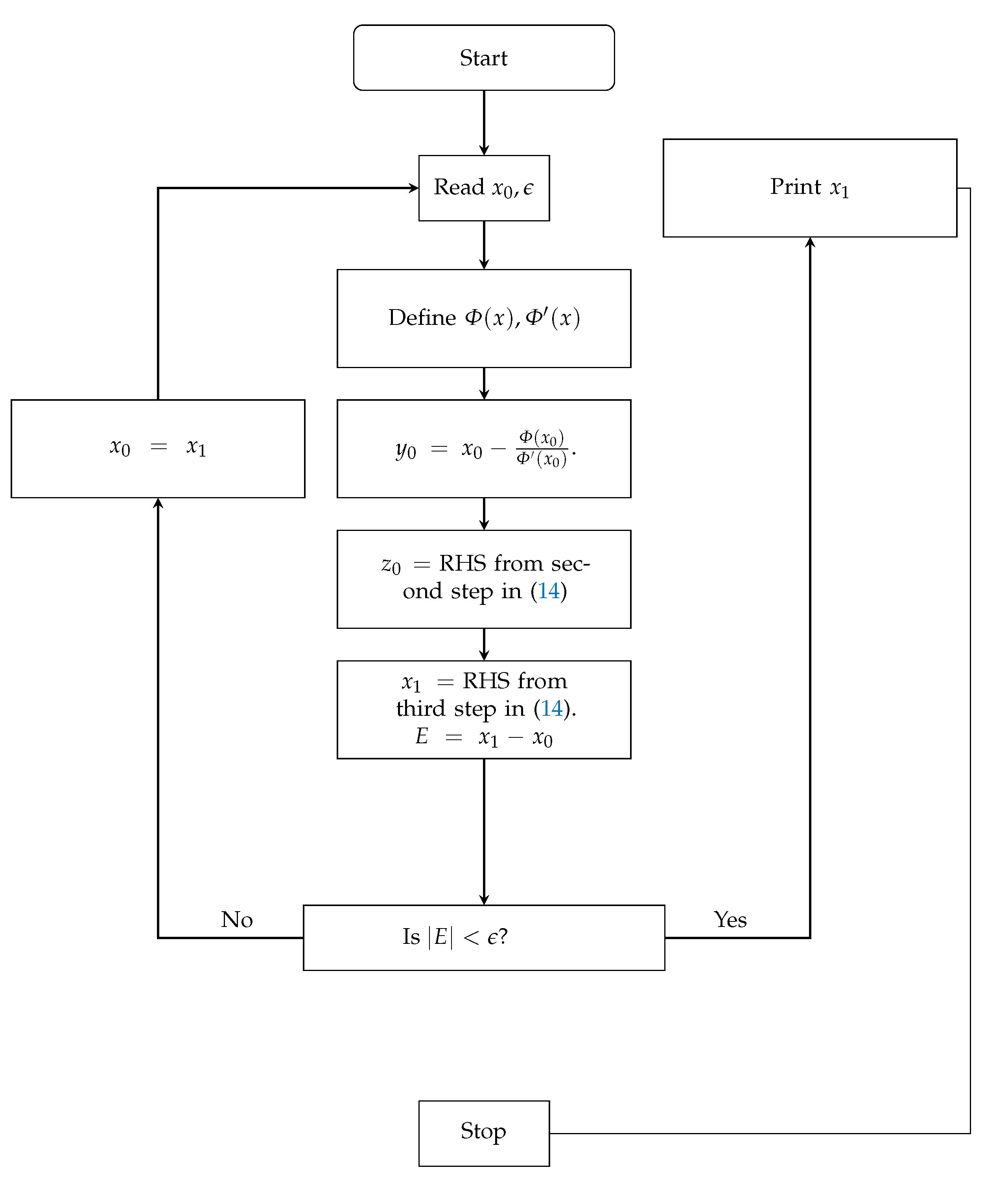
14) is abbreviated as PTNM, which stands for Proposed Taylor’s expansion-based Numerical Method. The flowchart of the above eighth-order proposed three-step iterative method is shown in
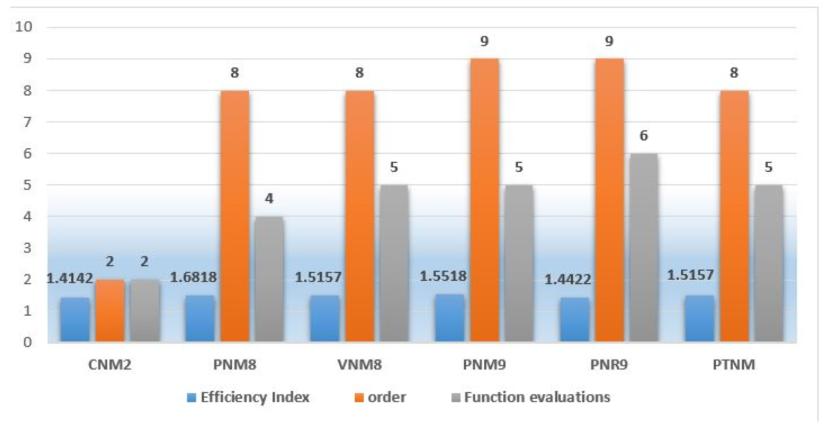
Figure 1. Moreover, the convergence order, the number of function evaluations per iteration, and the efficiency index of the proposed method are computed as 8, 5, and 1.5157, respectively. A comparative analysis of some methods under consideration based on these parameters is depicted in
Figure 2.
4. Convergence Analysis
When a convergence theorem for an iterative method claims convergence while presuming the existence of a solution
and a suitably chosen initial approximation close enough to
, it is referred to as a local convergence theorem. In contrast, a convergence theorem [
26] pp. 575–600, does not presuppose the existence of any solution a prior but instead presupposes that specific criteria are true at the beginning point. A semilocal convergence theorem is what it is termed.
This section has been devoted to proving the convergence analysis based on the assumption of the existence of at least eighth-order derivatives of
. The necessary order of convergence has been obtained through the application of Taylor’s series expansion with a single variable. It is important to note that the convergence analysis is approached in a manner that is comparable to that of a large number of other previously published publications and that the primary interest in the creation of higher-order methods is of an intellectual nature. Even if higher-order algorithms are more difficult to understand, their efficiency can be assessed; this is why we have included the CPU time, which can be found in
Section 6 of the article.
Theorem 1. Suppose that is the exact root of a differentiable function for an open interval Then, the three-step proposed method given in (14) has eighth-order convergence and the asymptotic error term is determined to be:where , and , Expanding
via series of Taylor about
, we obtain
Expanding
via series of Taylor about
, we obtain
Applying Taylor series for function
about
, we have
Multiplying (
16) and (
18), we obtain:
Substituting (
19) in the first-step of (
14), we obtain
where
. Using the Taylor’s series for
around
, we obtain:
Expanding
via series of Taylor about
, we obtain
Applying Taylor series for function
about
, we have
Multiplying (
21) and (
23), we obtain:
where
. Using the Taylor’s series for
around
, we obtain
Expanding the Taylor series using Equations (
17) and (
22), we obtain the expansion for the finite-difference quotient
S as follows:
Using the Equations (
16), (
18) and (
25) in the second step of the proposed method (
14), we obtain
Using the Equations (
16)–(
18), (
21)–(
23) and (
26) in the third step of the proposed method (
14), we obtain
The aforementioned equation demonstrates that the suggested approach (
14) converges to the eighth order.
5. Polynomiography: Fractal and Non-Fractal Images
Creative design and pattern development are two of the trickiest challenges in CAD. The process of creating patterns includes many different steps, such as analysis, creativity, and development. A designer must address all of these factors to create an engaging pattern that can be used in jewelry design, carpet design, tapestry design, etc. That is why it is so inspiring and practical to find novel ways to generate a wide range of fascinating patterns. Mathematical theory is one potential source for such procedures. As a type of mathematical object, polynomials have the potential to produce a wide range of interesting and lovely patterns. Polynomiography is commonly used to create patterns using polynomials.
Polynomiography is a method that combines mathematics with art to develop a new kind of visual art. The visuals that are produced are the outcome of an algorithmic visualization of repeated attempts to solve a polynomial problem. At the turn of the 21st century, Dr. Bahman Kalantari was the one who first articulated the meaning of this phrase [
27]. Dr. Bahman Kalantari’s research on polynomial root-finding served as the impetus for the development of the concepts of polynomiography. Polynomial root-finding is an age-old and time-honored field of study, but it never ceases to produce new insights with the advent of new generations of mathematicians and scientists. The term “polynomiography”, which is a combination of the words “polynomial” and the suffix “graphy”, was initially developed by Dr. Kalantari. A picture that was generated independently as a consequence of polynomiography is referred to as a “polynomiograph”. “An iterative process for constructing two-dimensional colored drawings (polynomiographs) that represent polynomials”, is how its definition reads.
Fractals are connected to polynomials via an area of mathematics known as polynomiography. Polynomiography is described as “the art and science of visualizing the zeros of complex polynomials utilizing fractal and non-fractal pictures formed using the mathematical convergence qualities of iteration functions. Instead of being a fractal image, a polynomiograph is a visual depiction of a polynomial’s roots. Finding the roots of small to intermediate degree polynomials has received a lot of research, while big polynomials have received less attention since they are less frequently encountered in mathematical studies. The fractal patterns that were created were different and could be used in many different ways, such as in the textile and ceramics industries.
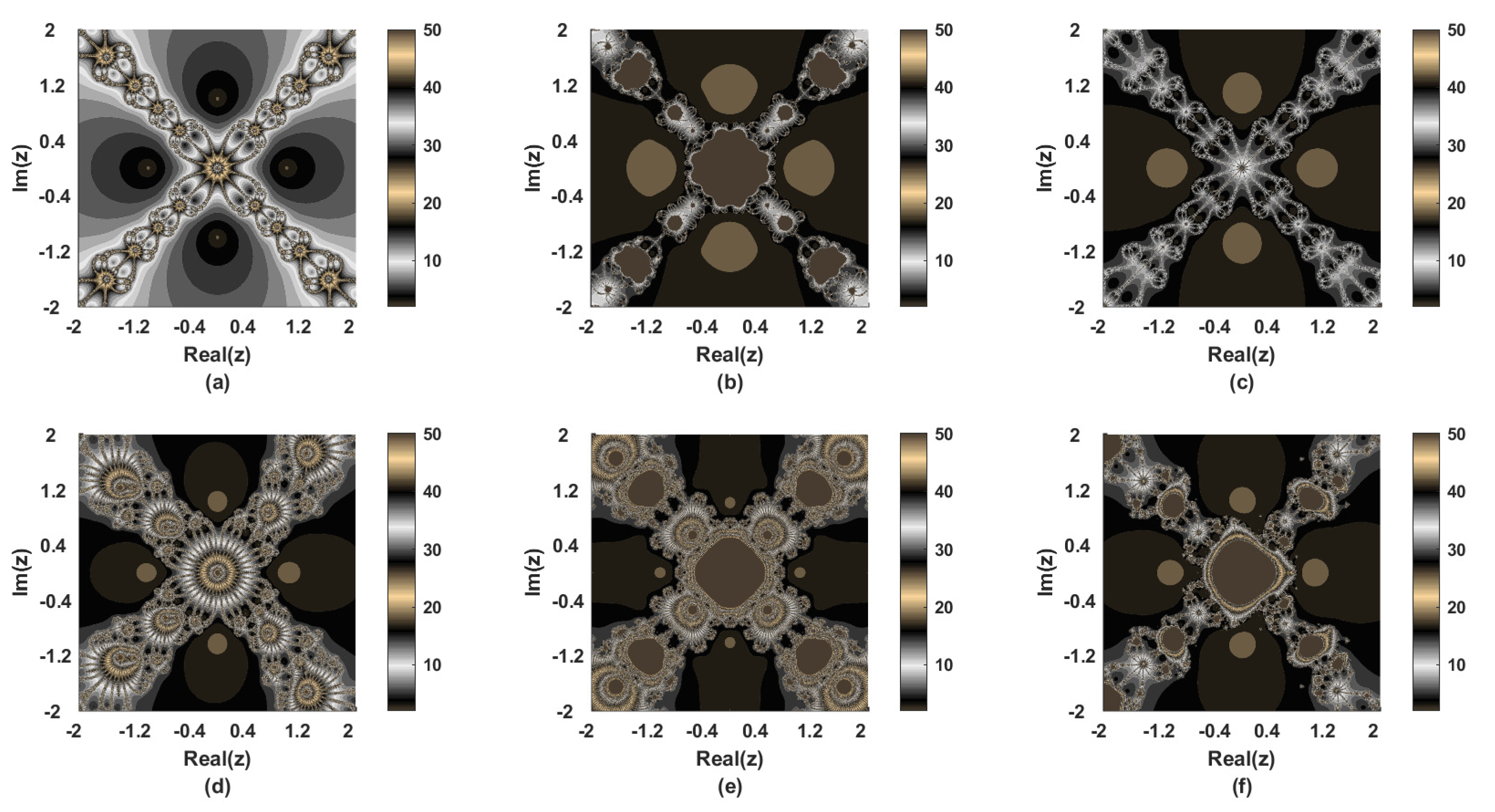
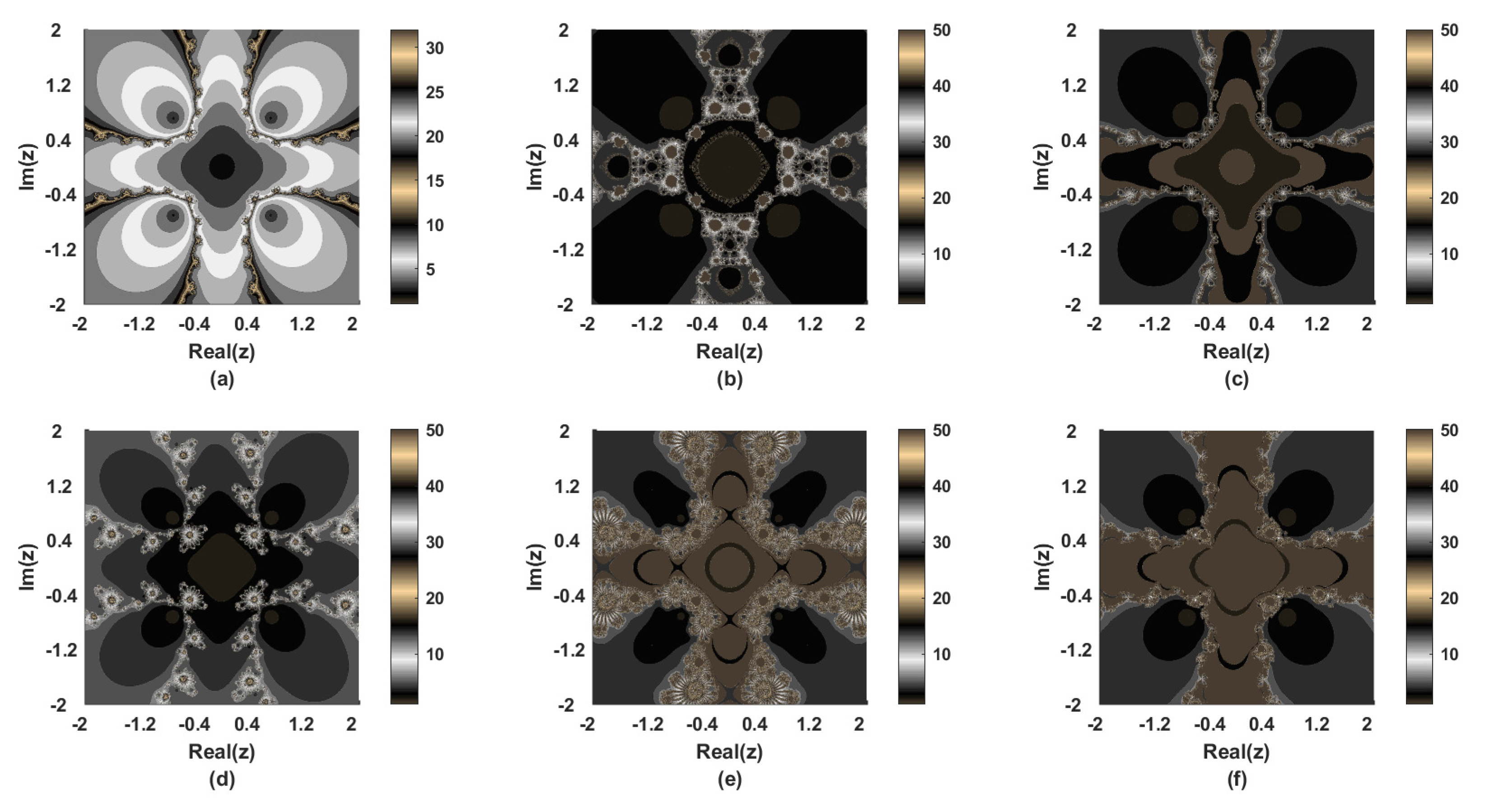
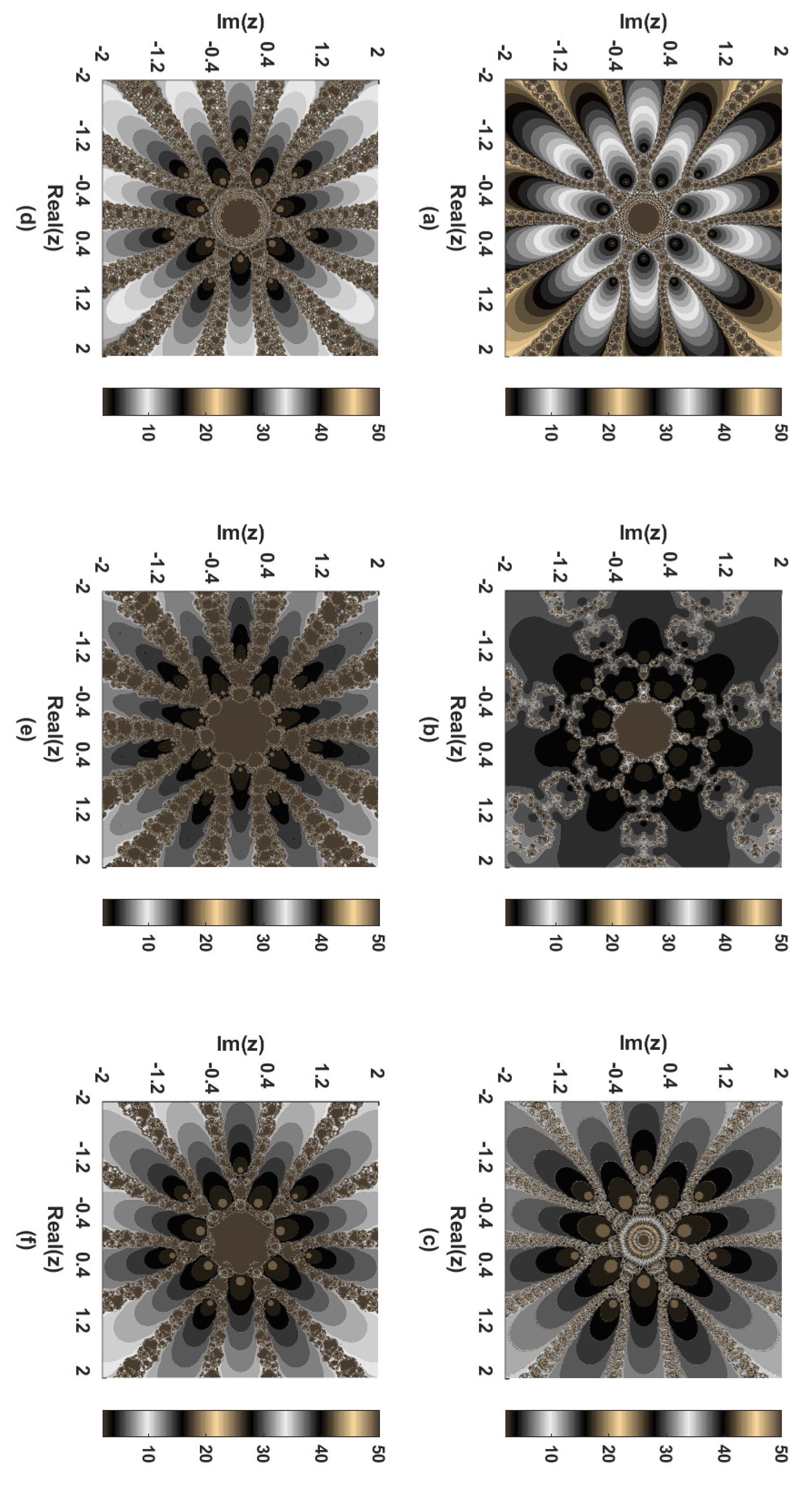
To generate polynomiographs over the complex plane
utilizing the computer program, we made use of a rectangle
R along with the dimensions
, and the maximum number of iterations of
with accuracy
. This was done by taking some complex polynomials as shown in Equation (
29). The areas of the image where the algorithm did not successfully converge have been assigned the color black. The pixel density of the produced visual representations is defined by the dividing of
R; for example, if we partition the rectangle
R into a grid of 2000, the plotting polynomiographs would have a higher resolution as a result. We used the following four complex polynomials including their roots (both real and complex) to show graphic elements in the complex plane:
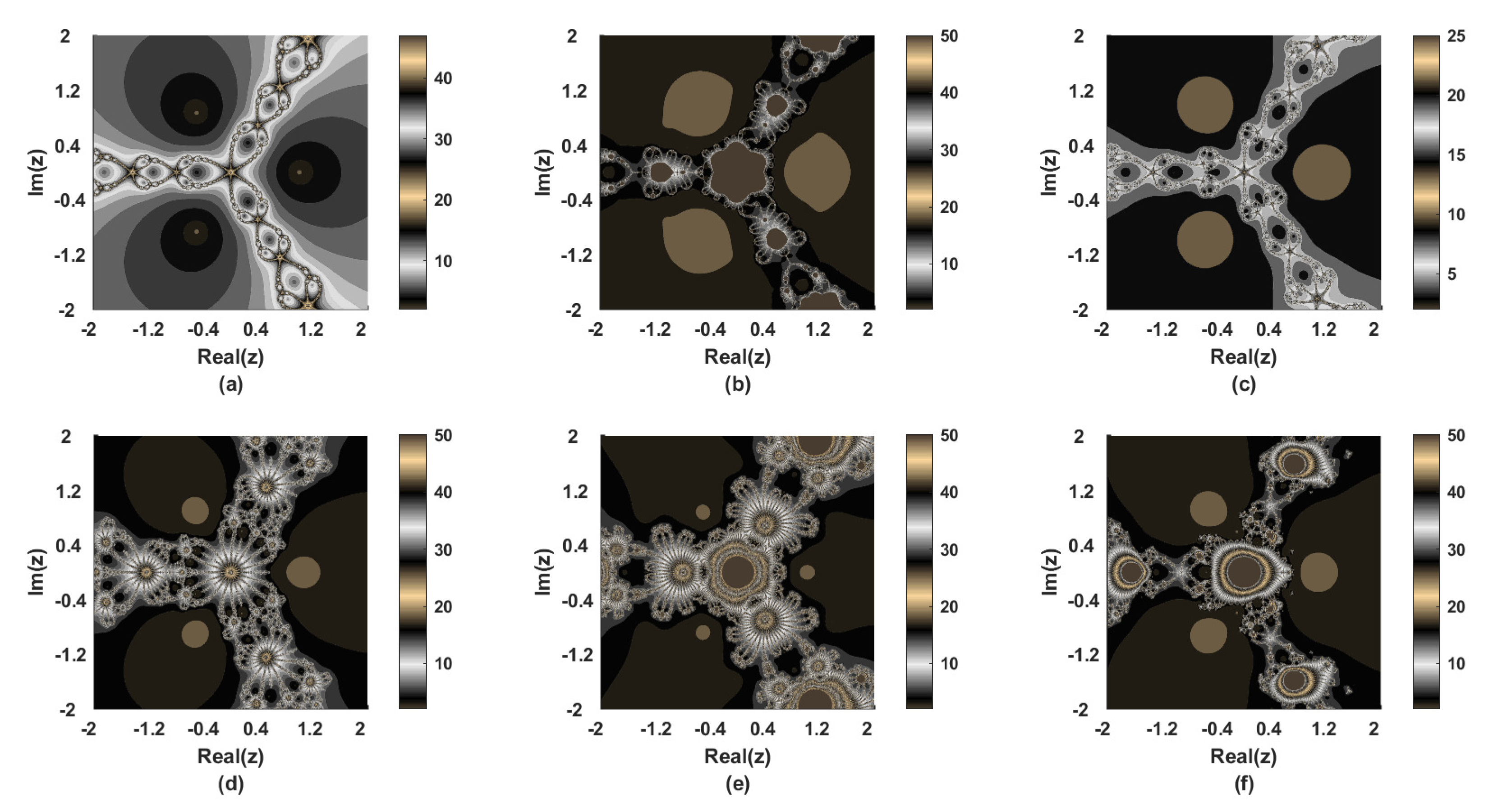
The images obtained are shown in
Figure 3,
Figure 4,
Figure 5 and
Figure 6 for the complex-valued polynomials given in Equation (
29), respectively while considering the iterative techniques as follows:
- (a)
Classical Newton Method of second order convergence in (
2).
- (b)
A method with eighth-order convergence in (
3).
- (c)
A method with eighth-order convergence in (
4).
- (d)
A method with ninth-order convergence in (
5).
- (e)
A method with ninth-order convergence in (
6).
- (f)
The proposed method with eighth-order convergence in (
14).
It is worth to be noted that in each Figure, plot (a) shows the fractal behaviour of the classical Newton Method of second-order convergence, plot (b) shows the fractal behaviour of the eighth-order method given in (
3), plot (c) shows the fractal behaviour of the eighth-order method given in (
4), plot (d) shows the fractal behaviour of the ninth-order method given in (
5), plot (e) shows the fractal behaviour of the ninth-order method given in (
6), and plot (f) shows the fractal behaviour of the proposed eighth-order method given in (
14). Darker regions in each plot indicate divergence regions that do not appear in fractal pictures generated using the suggested eighth-order approach. It demonstrates how, with a good first approximation, the approach can converge more quickly.
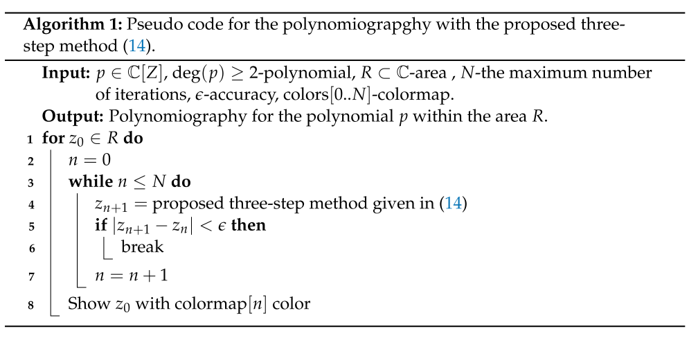
It may also be noted that the pseudo-code for the polynomiography via the proposed three-step method (
14) is given in Algorithm 1. It has been explained how the different coloring is assigned in some regions and how the colormap works in case of different colors and shadings within the phase planes of several complex polynomials under consideration. Pseudo-code offers a way to find polynomiographs. The proposed three-step procedure is iterated in the algorithm for each point in the region
under consideration. We assume the resulting sequence converges to a root of
p and stops iterating if the modulus of the difference between two successive points in the iteration process is less than the provided precision
. If the maximum number of cycles (
N) is reached, then the generated sequence is assumed to not converge to a root of
p. At the very end, we assigned a color to the location that was being considered by utilizing the colormap that was presented to us together with the iteration number when we exited the while loop.
![Symmetry 15 00330 i001 Symmetry 15 00330 i001]()
6. Physical Models for Numerical Simulations
In this section, we will conduct some numerical simulations to highlight the performance of the suggested iterative technique with eighth-order convergence, which is given in the equation. There are many distinct kinds of nonlinear functions that are taken into account. Only applicable nonlinear models, such as those used in medical science, healthcare, population dynamics, and blood flow, are discussed in this article in order to provide the findings with more support and credibility. We utilize the stopping criterion to determine when to end the number of iterations, where the tolerance is set to , and the needed accuracy is specified to be as high as 4000.
The following tabular representations of numerical results obtained from nonlinear practical models have been created, with each table containing an initial guess, a total number of function evaluations to achieve the tolerance, absolute error, the absolute value of the underlying function at the final approximated solution, and the amount of CPU time consumed by each approach, measured in seconds. The required numerical results were accomplished by using the program Mathematica 12.1 while operating under the Windows 10 operating system. The computer has an Intel(R) Core(TM) i7-1065G7 CPU running at a speed of 1.30 GHz. The installed memory was 24.0 GB.
Numerical Results and Discussions
Table 1,
Table 2 and
Table 3 show that the absolute error at the final iteration after simulating the chosen real models with the proposed method is the smallest of all the errors produced by other existing methods, as is the absolute functional value while consuming a reasonable amount of machine time measured in seconds. The number of function evaluations required by PTNM is appropriate for the first assumptions and, in some cases, it outperforms higher-order approaches. In addition, it is important to highlight that the suggested technique does not contain any aspects of divergence, in contrast to certain current methods, which do have such elements, as shown in
Table 3. In conclusion, it has been demonstrated that the procedure described in (
14) is applicable in a variety of real-life and physical circumstances where one must interact with a nonlinear phenomenon.
Problem 1. We have taken a blood rheology nonlinear model from [4] as shown below:where x shows the plug flow of Caisson fluid flow. Caisson fluid is used to represent blood despite the fact that it is a non-Newtonian fluid. The Caisson fluid model hypothesizes that a simple fluid like water or blood will move through a tube in such a way that its central core will move as a plug with very little distortion and that a velocity gradient will develop along the tube’s walls. It may be noted that the blood comes under the category of Caisson fluid. The numerical simulations for the model (30) are presented in Table 1. Problem 2. Law of Blood Flow [
5]:
where and are chosen for the simulations with being the distance to be determined. With these parameters, the above model turns out to be
where
stands for the radius of the fiber,
p shows the specific hydraulic permeability, and
is the porosity of the medium. If we assume
and
, we obtain the following third-degree polynomial:
The numerical simulations for the model (
33) are presented in
Table 2.
Problem 3. In the study of population dynamics, one of the models that is utilized most commonly is the mathematical representation of population growth, referred to as the population growth (PG) model. Using a first-order ordinary differential equation, the following expression can be used to describe the model:where stands for the population growth at time t, κ shows the constant birth rate while ν is for constant immigration rate. The above linear ordinary differential equation has the following closed-form solution:where is the population at (initial population). In one particular piece of research, the problem is stated as follows: Let us say that a particular community had a starting population of 1,000,000 people, that 435,000 people immigrated into the community in the first year, and that the town had a total population of 1,564,000 people by the conclusion of the first year. Determine the rate of births in this population. Using the initial condition and values of the other parameters given as stated, the birth rate κ can be determined with the help of the following nonlinear equation which is the closed-form solution of the model (34) after applying the stated situation:where is the required birth rate. The numerical simulations for the model (36) are presented in Table 3. 7. Concluding Remarks and Future Directions
The success of this investigation hinges on the development of a brand-new iterative strategy that converges at the eighth-order level after three iterations. The projected computational order of convergence is consistent with the theoretical demonstration of convergence provided by Taylor’s series expansion for nonlinear equations. Thus, the PTNM method can be applied to problems with either a single nonlinear equation or a system of such equations. In addition, dynamical aspects of PTNM can be investigated using basins of attraction, which, when applied to complex-valued functions, yield aesthetically pleasing phase plane diagrams. This demonstrates the method’s validity for making first estimates that are statistically very close to the underlying nonlinear model. We also get polynomiographs that are both aesthetically pleasing and intellectually stimulating. The real values of parameters have a symmetrical effect, but the imaginary values of parameters distort polynomials. In the end, some medically-relevant nonlinear equations were applied to PTNM and other well-known optimum and non-optimal techniques in the sense of King–Traub. It has been found that PTNM yields better results than other methods in the vast majority of cases. This is notably the case concerning the N-th iteration threshold for achieving the target precision, error, and functional value. It is also worth noting that the proposed method will always converge, regardless of how close to or far from the starting guess the approximate solution is. Remembering this is essential. The PTNM algorithm converges to the eighth order and is an iterative method that can compete with other algorithms. It can be used to find solutions to nonlinear systems and equations.
As far as we can tell, high-order approaches are solely of interest in the academic community since very precise approximations to answers are not needed in most real-world contexts. However, these methods are rather complex and do not significantly increase productivity relative to simpler alternatives. The method proposed here is also one of the memory-free techniques discussed in the article. In the case of nonlinear systems, it also requires the evaluation of additional Jacobian matrices, which increases the computing burden. To reduce the computational complexity of the current method, we plan to make a change in future research by proposing a finite-difference approximation for the first-order derivative. We will also look more closely at the proposed method to see if it has semi-local convergence and better visualization with a variety of convergence tests including distance and non-distance conditions over different types of metrics. In addition, the three-step numerical solver that was proposed can be extended to the concept of fractional calculus [
28], in which the traditional derivative is replaced by the fractional Riemann–Liouville or Caputo derivatives. This allows the solver to be used to solve problems involving fractional calculus.
