Abstract
The reconstruction of the geometry of weld-deposited materials plays an important role in the control of the torch path in GMAW. This technique, which is classified as a direct energy deposition technology, is experiencing a new emergence due to its use in welding and additive manufacturing. Usually, the torch path is determined by computerised fabrication tools, but these software tools do not consider the geometrical changes along the case during the process. The aim of this work is to adaptively define the trajectories between layers by analysing the geometry and symmetry of previously deposited layers. The novelty of this work is the integration of a profiling laser coupled to the production system, which scans the deposited layers. Once the layer is scanned, the geometry of the deposited bead can be reconstructed and the symmetry in the geometry and a continuous trajectory can be determined. A wall was fabricated under demanding deposition conditions, and a surface quality of around 100 microns and mechanical properties in line with those previously reported in the literature are observed.
1. Introduction
The industry is moving in the direction of the assumption of concepts such as Industry 4.0—Internet of Things (industry of the future), which makes traditionally manual processes, such as welding technologies, adopt smart solutions that have ecological benefits, productivity, traceability, and are quality-oriented to improve the manufacturing and production stages [1]. Efforts are being made by researchers to develop intelligent and sensorised automated systems. To predict and control the quality of the welding process, integrated systems for detection, monitoring, and control have been developed [2]. Recent developments in monitoring have included the adoption of various techniques for both melt-pool control and layer geometry [3]. It is generally based on the inclusion of a process measurement sensor [4] and the application of either an artificial intelligence (AI) or process intelligence technique [5]. Table 1 summarises some of the sensors used for geometry determination in deposition processes for welding and additive manufacturing. It can be seen from the table that there are two vision technologies: CCD (Charge-Coupled Device) sensors, which have been previously widely used for machine vision, are losing some attraction to the more modern CMOS (Complementary Metal–Oxide Semiconductor) image sensors [6].

Table 1.
Sensors and measurement entity in welding and additive manufacturing.
The right choice of measurement technology and the use of sensor fusion algorithms combined with indirect measurement methods can help to reduce welding production costs and increase productivity by detecting or predicting many welding defects or deviations from set points [17]. These measurements make it possible to adjust the welding current source and robot parameters online in a closed-loop control. The online evaluation of unmeasured variables improves control systems and reduces the number of rejected parts in the final quality inspection.
To take advantage of modern welding power sources, it is important to equip the monitoring system with serial communication. The modelling of the estimator is an essential step to obtain an accurate measurement system and, due to the thermal inertia of the process, a dynamic model is more representative of the welding process than a static one. Visual and thermal imaging techniques, image processing, and neural network algorithms, although computationally more resource-intensive, are the most widely used for estimating weld bead geometry and excellent results have been observed. More and more research is being conducted on sensor fusion algorithms. Following this trend, this paper presents a new modelling approach that uses arc weld measurements and thermal imaging information to create a dynamic model for weld penetration estimation. This new method obtains information about the amount and spatial distribution of energy in the subject and uses only additive operations, which simplifies calculations and improves model accuracy. Using it to control welding automation with a computer or integrated equipment provides a satisfactory solution.
Although much has been published, especially in the characterisation of materials, joints, transfer modes, process selection, and inspection methods, process monitoring is something that is still being worked on and requires attention [18]. In this direction, in addition to the monitoring of the correct deposition and process status, the optimisation of weld paths based on online measurement is an issue that can improve automated welding applications and help the incorporation of easy-to-manufacture applications in direct energy deposition (DED) additive manufacturing. These DED, when using a filament and an arc as a generator, are called WAAM [19]. Many of the WAAM applications that deal with a trajectory definition often deal with the definition of parameters and trajectory patterns for area filling (so-called slicing) [20]. In addition, since the paths are designed for different components, the working paths applied may affect the quality of the weld and the weld [21]. However, in general, these developments focus on solutions for specific T-junction types [22], cross intersection [23,24], and specific geometries [25]. This paper covers the gap of considering interlayer growth and considers layer symmetry.
Furthermore, the use of symmetry as a phenomenon inherent to the nature of deposition in this type of process has been little explored [26]. This paper aims to correctly select the trajectory based on the measurement of the previous layer. The main novelty presented is the incorporation of a robot-integrated sensor for layer estimation in Gas Metal Arc Welding (GMAW) and an analytic based on mass balance and symmetric calculations for the correct estimation of the trajectory in the consecutive pass.
2. Materials and Methods
This section describes the equipment used and the most significant welding parameters. It also includes a second subsection that briefly describes the architecture of the measuring equipment used and their communication. Finally, the treatment of the profile acquired by the sensor installed on the welding robot is described.
2.1. Materials and Set-Up
The welding tests were carried out using a robotic-fixed table welding system. The welding equipment used has an Alpha Q 552 pulse current generator (EWM, Mündersbach, Germany), which uses GMAW technology and powers the torch. The torch movement is managed by a special anthropomorphic Fanuc Arc Mate 100-iC reference welding robot (Fanuc, Oshino, Japan). In addition to generation and movement, the torch must be fed with metal wire by means of a wire feed unit from EWM (Mündersbach, Germany) with reference M drive 4 Rob5 XR RE and a shielding gas system. A Queltech Q4-120 profilometer (München, Germany) is also equipped to measure the geometry of the interlayer bead. It is positioned perpendicular to the substrate and its movement is analogous to that of the torch in the weld. Table 2 summarises the characteristics of the laser profilometer for the measurement of the weld layer profile.
Table 2.
Characteristics of the Queltech Q4-120 laser profilometer.
Among the modes used in GMAW welding, the synergic pulse mode is one of the most widely used variants of welding equipment. In order to perform the pulse current train correctly, it is necessary that the welding equipment has a digitally controlled synergic generation source. The pulses control the melting of the material for the generation of the droplet and the final detachment of the droplet. This material is subsequently fused to either the substrate or the underlying layer. The generation parameters of the welding equipment (peak/background current, peak duration, base duration, pulse frequency, etc.) are matched and related to the process parameters (type of material and wire diameter and shielding gas) and are unique to the selected wire speed. These calculations are collected in a database for each material and include calculation routines. The uniformity of the profile and penetration of the weld bead is therefore the objective of the application of these synergic modes. Figure 1 shows the experimental set-up and the arrangement of the laser in the measurement of the welded layer.
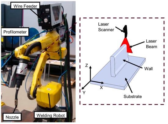
Figure 1.
Experimental set-up and solder layer scanning process.
The material used for the welding tests was a mild steel commonly used in many industrial applications, and its name is ER70S-6 steel. This material was deposited in the form of commercially produced 1.2 mm diameter wire. The composition by weight percentage is shown in Table 3. This information was provided by the supplier. As the substrate material, S235JR steel was used in the form of steel plates with a thickness of 10 mm.
Table 3.
Chemical composition in weight % of ER70S-6 wire.
Table 4 shows a summary of the parameters used for the achievement of the GMAW weld layers. The welding was carried out with the torch in a vertical position, perpendicular to the base (substrate). The distance at which the wire exits the welding contact tip (stick-out) was 22 mm. The shielding gas was a mixture of argon and carbon dioxide (20% CO2 and 80% Ar) with a flow rate of 17 L/min. These gas supply conditions were used according to the welding equipment supplier’s guidelines for the material used. These parameters had already been optimised for the use of this material on this substrate in previous papers.
Table 4.
Relevant parameters for the welding process.
2.2. Data Measurement Chain in the Robotic GMAW Process
The data measurement chain necessary to implement the methodology described in this paper is shown in Figure 2. The source data had two main sources: the robot control from which the robot position data, execution program, power source generation data, and wire speed data are extracted, and the profilometric laser, which has its own coordinate axis on which the point cloud describing the 2D profile of the welded layer will be extracted. These data are transferred to a server PC in which the communication node makes possible the integration of all the information ensuring the synchronisation of the data. This server PC will be used to run the algorithm and return the corrected and optimised motion execution program. All this was developed using Robot Operating System (ROS) tools. Additionally, the server feeds a database for access to the information once the live cycle is performed and a GUI (Graphical User Interface) in a mobile or tablet application that allows the operator to access profiles and to know points of the trajectory on the acquired profiles.
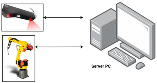
Figure 2.
Hardware and communication for data acquisition of the GMAW process.
2.3. Point Cloud Preparation and Processing
The raw signal that is captured by the laser profilometer must be suitable for use in the methodology described in this paper. Some of the sources of noise in the point cloud originate from surface glare and dirt, so filtering and conditioning of the data are necessary.
The treatment follows three stages, as can be seen in Figure 3. They are as follows:
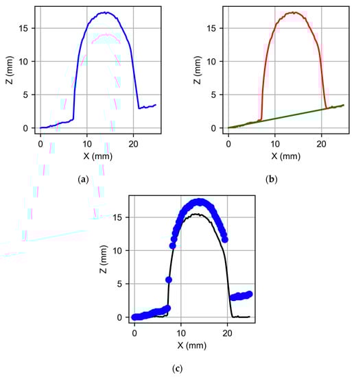
Figure 3.
Stages in profile processing: (a) raw signal, (b) skew removal, and (c) final interpolated profile for the use of the algorithm.
- The layer profile is translated to 0 at its extreme point (see Figure 3a).
- The profile is filtered to remove brightness with a moving median filter of order N = 7. The trend of the signal is removed to eliminate the positioning error of the substrate, which in this case is eight degrees. This removed angle then allows the torch to be placed perpendicular to the substrate, which is desired (see Figure 3b).
- Once the tilt is corrected by means of an interpolation, a greater number of points in the cloud are extracted by means of a Piecewise Cubic Hermite Interpolating Polynomial (pchip) interpolation because it adjusts the flat areas more adequately than the interpolation by splines (see Figure 3c).
3. Results
In the Results Section, the application of different methodologies to obtain the optimal flare trajectory is described. The algorithm is based on a first calculation of the centroid of the deposited layer; then, the symmetry point of the profile is calculated and, finally, the trajectory that optimally compensates the growth of the layer is generated.
3.1. Methodology Based on Centroid Calculation
For the calculation of the centroid, the profile was considered as a continuous function, where the height position z depends on the transverse position x, this continuous function z(x) being in the measuring interval of the profilometer x = 0 to x = xmax. In this interval, the area under the curve of the function z(x) is calculated as the following integral (Equation (1)).
The function has a paraboloid shape and its area under the curve is described by an S-shape typical of sigmoid functions, as it can be seen in Figure 4a. The objective is to find the point xi where the AUC(xi) is equal to half the total area:
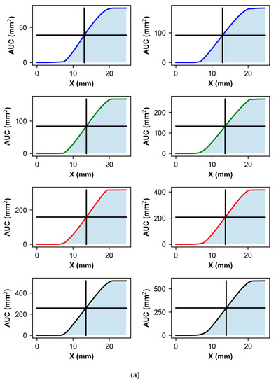
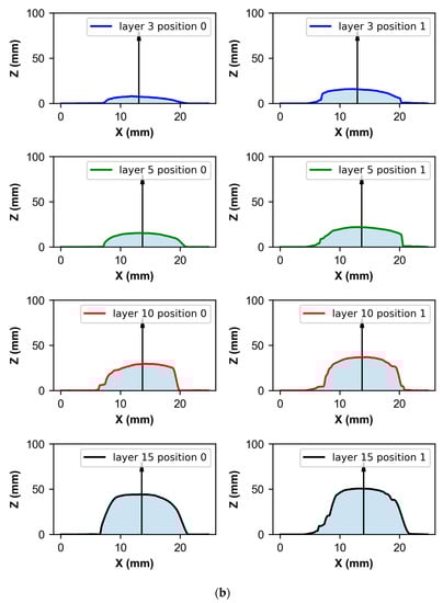
Figure 4.
Calculation of the (a) area under the curve and (b) centroid in the selected profiles and layers.
The midpoint of this region was taken as the centroid (xi) to be considered for the further study of the symmetry of the profile in the layer. The scanned profile and the calculated centroid for different layers and profiles within the layer can be seen in Figure 4b.
In the first layers, the profile obtained by means of the scanner is not determinant for the generation of a correct profile for the calculation of the centroid but more in the case of the symmetry, so the first two layers are discarded. In these layers, the symmetry calculation is based more on the arrangement of the substrate than on the proper geometry of the deposited layer profile.
3.2. Methodology Based on Symmetry Calculation
The approach for the calculation of the torch position is simple. We looked for the point of maximum layer symmetry around the point calculated in the previous section of the centroid. For the calculation of the symmetry, we used a similar approach to the one used by Veiga et al. [27] for the calculation of the symmetry of the previous layer for the definition of the trajectory of the next layer.
The function z(x) was assumed, where z is the position of the point taken from the laser profilometer, starting from the centroid in a close interval between z(xi – 0.6) and z(xi + 0.6). The point xi was calculated as explained in Section 3.1. At the different points of that interval, the symmetric function zs(x) and the antisymmetric function zas(x) are calculated according to the following equations:
The symmetry and antisymmetry function were evaluated as described above in a section close to the centroid to obtain the point of maximum symmetry. It can be seen later, then, that due to the shape of the symmetry, this interval does not necessarily have to be large. In Figure 5a,c, we can see the symmetric and antisymmetric functions at the most extreme points of the analysis section. It can be seen that the greatest asymmetry occurs at the limits of the layer with the substrate. Figure 5b shows the value of x, where the greatest symmetry occurs between the two sides of the layer profile.
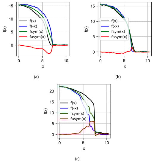
Figure 5.
Characteristic functions for the calculation of the symmetry around the centroid in x positions (a) −6 mm, (b) optimal point, and (c) 6 mm in the 5th layer of profile 1.
The symmetric function is close to the functions around the evaluation value x and the asymmetric function is closest to zero when the evaluation function z(x) is highly symmetric around the evaluation point xe. To quantitatively measure the symmetry according to [28], a coefficient characterising the symmetry was defined, where the coefficient C is calculated as
Figure 6a shows the value of the coefficient C as a function of the equation position xe around the centroid xi. C = 1 corresponds to pure symmetry and C = 0 when we have pure asymmetry. Figure 6a shows how the point of maximum symmetry is close to the centroid, which is consistent since the geometry of the deposited layer is intrinsically symmetric, as mentioned in several previous papers [29,30,31]. Figure 6b shows an example of four layers in two different positions; the arrow shows the centroid origin point and the dotted line (very close and easier to observe in Figure 6a) is the position of the point of maximum symmetry.
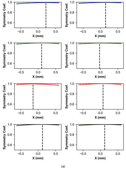
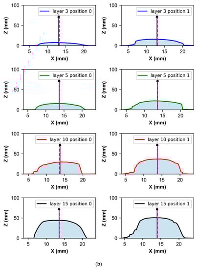
Figure 6.
Calculation of the (a) symmetry coefficient and (b) optimal symmetrical point in the selected profiles and layers.
3.3. Methodology Based on Symmetry Calculation
Finally, this section describes the methodology used to choose the trajectory of the torch. The premise is to maintain the length of the layer while keeping its point of maximum symmetry at the point closest to the point of mass distribution (centroid). For this purpose, the point that defines the trajectory in the profile is the point equidistant to the position relation between the point of maximum symmetry and the point of the centroid in the opposite direction. Once the points of the two-dimensional profiles are joined longitudinally, the three-dimensional trajectory of the torch is obtained, which ensures greater symmetry of the next layer. Figure 7 shows the average centroid of the wall and, in green, the point of optimal trajectory of the torch. The points in blue are those of maximum symmetry for 4 different layers in their zenithal view.
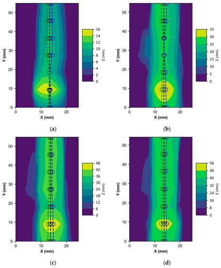
Figure 7.
Calculation of the trajectory, in green, as a function of the symmetry, in blue, around the centroid, in black, for the layers: (a) 3, (b) 9, (c) 12, and (d) 15.
4. Discussion
As a consequence of the application of the methodology described in this paper, it was possible to avoid excess material in areas that create imbalances in the wall and the material melts on the side of the solidified material. Figure 8a shows a sequence of welded layers in which the wall is poured to the side. On the other hand, Figure 8b shows the weld made by applying the described methodology with the same welding conditions. The trajectory correction significantly improved the deposition of the material.
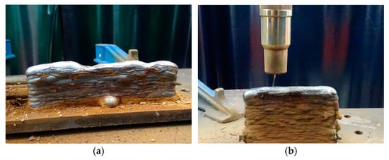
Figure 8.
Walls manufactured with the (a) constant centre and (b) symmetric algorithm developed in this paper.
Once the deposited wall was observed under poor growth conditions (Figure 8a), this effect could perhaps be overcome by acting on the generation signal or by modulating the deposition parameters, perhaps by lowering the deposition ratio of the wire speed to the feed rate. This wall could not be analysed to draw conclusions about the mechanical properties. In additive arc manufacturing, components are normally produced by applying several layers. The residual stress values in the component change as the multilayer deposition process progresses [21,32,33]. The proper deposition and symmetrical growth of the layers allows the better evaluation of the residual stress distribution. Therefore, only the wall manufactured with the nozzle trajectories established by the methodology described in this paper (Figure 8b) is analysed at this point.
The mechanical and metallographic characterisation of the mild steel walls produced using the algorithm described in this paper is briefly described. The wall analysis was performed on the basis of the horizontal macroscopic image of the wall. The edges of the walls were obtained by analysing the grey images with a Gaussian filter and studying the illumination (Figure 9b), following the method described by Artaza et al. [34]. The relevant standard DIN EN ISO 6892-1—Tensile testing of metals at room temperature was followed in the fabrication of test specimens. We used a saw to remove three sections of the wall and machine a cylinder with a core diameter of 4 and a metric M-6 threaded-end vertically parallel to the wall, as it can be seen in Figure 9a. The objective was to analyse the mechanical properties of the wall in the most critical directions, knowing that the material has similar values in the different test directions, but slightly worse in the vertical direction [35].
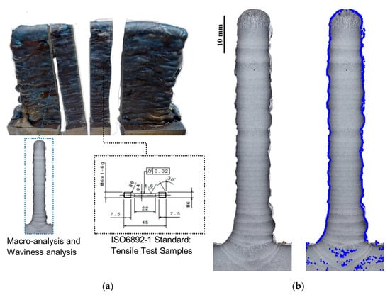
Figure 9.
Mechanical tests on the specimen manufactured by WAAM: (a) extraction of the specimens and (b) calculation of wall geometry.
As can be seen in Figure 10a,b, the wall has typical layer-by-layer deposition waviness in the centre of the wall where the surface is analysed. The wall surface profile is provided in terms of waviness parameters because it is impractical to determine roughness values for this type of analysis. Note that both wall surfaces find an equilibrium between the maximum and minimum values, indicating that the wall is compensated. The stress–strain graph of the three specimens tested in the vertical direction of wall growth is shown in Figure 10c. The curve shows the typical phases of a mild steel curve with yielding, strain hardening, and final necking.
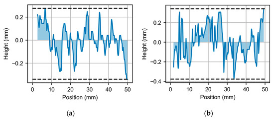
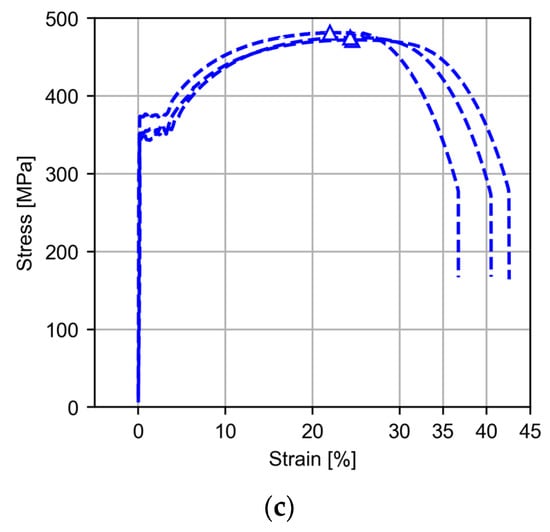
Figure 10.
Walls surface profile of the WAAM part on (a) left side (b) right side, and (c) strain–stress curve of tensile testing for WAAM mild steel.
From Figure 10a,b, the waviness indicators in the middle section of the wall can be seen. Both the area closest to the substrate and the area of the last layers were discarded. Table 5 presents a summary of the main key corrugation indicators for both sides of the wall. The waviness values are similar on both sides of the face. It is also good that the arithmetic mean of the waviness is in the micron resolution with values close to 100 µm.
Table 5.
Summary of the main key indicators (in mm) of waviness for both sides of the wall.
Table 6 shows the values of UTS (Ultimate Tensile Strength), YS (Yield Strength), and Elongation at fracture (Elong) in the vertical direction. The values are acceptable within those previously reported in the literature [18,19,21,35].
Table 6.
Summary of the mechanical properties of the WAAM mild steel wall.
5. Conclusions
This paper presented a methodology for the correct trajectory definition that avoids material detachment and ensures correct material deposition, applicable to both GMAW welding and additive manufacturing by the same technology. Some of the conclusions that emerged from this research are as follows:
- By using a profilometric scanner, the geometry of the layer was obtained to determine the centroid that divides the deposited material into two equal parts.
- The maximum symmetry point and the symmetry of the layer were also obtained. In itself, this result allows us to establish a control of the process, detecting early on deviations with respect to the correct development of the process.
- By means of the symmetry point and the centroid, a methodology for the definition of the interlayer trajectory was established that allows us to compensate for a deviation from the incorrect layer growth.
- The surface quality of the demo wall was analysed, and it has an average ripple of 126 microns on one side and 98 microns on the other side.
- This methodology was applied to the fabrication of an ER70-6 mild steel multi-layer wall with correct growth and compared to welding without the application of the methodology, thus improving the process in cases of high deposition rate.
- As a future line of research, it would be of interest to extend the application of this methodology to more complex parts or to welds in different types of joints.
Author Contributions
Conceptualization, F.V. and A.S.; data curation, D.C. and F.V.; formal analysis, D.C. and F.V.; investigation, F.V. and A.S.; methodology, D.C. and F.V.; project administration, A.S. and PV; supervision, A.S.; validation, D.C.; writing—original draft, D.C. and F.V.; writing—review and editing, D.C., P.V. and A.S. All authors have read and agreed to the published version of the manuscript.
Funding
This research received no external funding.
Data Availability Statement
The data presented in this study are available on request from the corresponding author.
Conflicts of Interest
The authors declare no conflict of interest.
References
- Gyasi, E.A.; Kah, P.; Penttilä, S.; Ratava, J.; Handroos, H.; Sanbao, L. Digitalized Automated Welding Systems for Weld Quality Predictions and Reliability. Procedia Manuf. 2019, 38, 133–141. [Google Scholar] [CrossRef]
- Liu, Y. Toward Intelligent Welding Robots: Virtualized Welding Based Learning of Human Welder Behaviors. Weld. World 2016, 60, 719–729. [Google Scholar] [CrossRef]
- Kah, P.; Shrestha, M.; Hiltunen, E.; Martikainen, J. Robotic Arc Welding Sensors and Programming in Industrial Applications. Int. J. Mech. Mater. Eng. 2015, 10, 13. [Google Scholar] [CrossRef]
- Garašić, I.; Kožuh, Z.; Remenar, M. Sensors and Their Classification in the Fusion Weldingtechnology. Teh. Vjesn. 2015, 22, 1069–1074. [Google Scholar] [CrossRef]
- Bestard, G.A.; Sampaio, R.C.; Vargas, J.A.R.; Alfaro, S.C.A. Sensor Fusion to Estimate the Depth and Width of the Weld Bead in Real Time in GMAW Processes. Sensors 2018, 18, 962. [Google Scholar] [CrossRef] [PubMed]
- Tejas, R.; Macherla, P.; Shylashree, N. Image Sensor—CCD and CMOS. In Microelectronics, Communication Systems, Machine Learning and Internet of Things; Nath, V., Mandal, J.K., Eds.; Springer Nature: Singapore, 2023; pp. 455–484. [Google Scholar]
- Ding, D.; He, F.; Yuan, L.; Pan, Z.; Wang, L.; Ros, M. The First Step towards Intelligent Wire Arc Additive Manufacturing: An Automatic Bead Modelling System Using Machine Learning through Industrial Information Integration. J. Ind. Inf. Integr. 2021, 23, 100218. [Google Scholar] [CrossRef]
- Wang, C.; Bai, H.; Ren, C.; Fang, X.; Lu, B. A Comprehensive Prediction Model of Bead Geometry in Wire and Arc Additive Manufacturing. J. Phys. Conf. Ser. 2020, 1624, 022018. [Google Scholar] [CrossRef]
- Li, F.; Chen, S.; Shi, J.; Zhao, Y.; Tian, H. Thermoelectric Cooling-Aided Bead Geometry Regulation in Wire and Arc-Based Additive Manufacturing of Thin-Walled Structures. Appl. Sci. 2018, 8, 207. [Google Scholar] [CrossRef]
- Tang, S.; Wang, G.; Huang, C.; Zhang, H. Investigation and Control of Weld Bead at Both Ends in WAAM. In Proceedings of the 30th Annual International Solid Freeform Fabrication Symposium—An Additive Manufacturing Conference, Austin, TX, USA, 12–14 August 2019. [Google Scholar]
- Karmuhilan, M.; Sood, A.K. Intelligent Process Model for Bead Geometry Prediction in WAAM. Mater. Today Proc. 2018, 5, 24005–24013. [Google Scholar] [CrossRef]
- Pradhan, R.; Joshi, A.P.; Sunny, M.R.; Sarkar, A. Performance of Predictive Models to Determine Weld Bead Shape Parameters for Shielded Gas Metal Arc Welded T-Joints. Mar. Struct. 2022, 86, 103290. [Google Scholar] [CrossRef]
- Bi, G.; Sun, C.N.; Gasser, A. Study on Influential Factors for Process Monitoring and Control in Laser Aided Additive Manufacturing. J. Mater. Process. Technol. 2013, 213, 463–468. [Google Scholar] [CrossRef]
- Wang, D.; Wu, S.; Fu, F.; Mai, S.; Yang, Y.; Liu, Y.; Song, C. Mechanisms and Characteristics of Spatter Generation in SLM Processing and Its Effect on the Properties. Mater. Des. 2017, 117, 121–130. [Google Scholar] [CrossRef]
- Colodrón, P.; Fariña, J.; Rodríguez-Andina, J.J.; Vidal, F.; Mato, J.L.; Montealegre, M.Á. Performance Improvement of a Laser Cladding System through FPGA-Based Control. In Proceedings of the IECON 2011—37th Annual Conference of the IEEE Industrial Electronics Society, Melbourne, VIC, Australia, 7–10 November 2011; pp. 2814–2819. [Google Scholar]
- Chabot, A.; Rauch, M.; Hascoët, J.-Y. Towards a Multi-Sensor Monitoring Methodology for AM Metallic Processes. Weld. World 2019, 63, 759–769. [Google Scholar] [CrossRef]
- Bestard, G.A. Online Measurements in Welding Processes; IntechOpen: London, UK, 2020; ISBN 978-1-83881-896-8. [Google Scholar]
- Srivastava, M.; Rathee, S.; Tiwari, A.; Dongre, M. Wire Arc Additive Manufacturing of Metals: A Review on Processes, Materials and Their Behaviour. Mater. Chem. Phys. 2023, 294, 126988. [Google Scholar] [CrossRef]
- Tripathi, U.; Saini, N.; Mulik, R.S.; Mahapatra, M.M. Effect of Build Direction on the Microstructure Evolution and Their Mechanical Properties Using GTAW Based Wire Arc Additive Manufacturing. CIRP J. Manuf. Sci. Technol. 2022, 37, 103–109. [Google Scholar] [CrossRef]
- Ding, D.; Pan, Z.; Cuiuri, D.; Li, H. A Tool-Path Generation Strategy for Wire and Arc Additive Manufacturing. Int. J. Adv. Manuf. Technol. 2014, 73, 173–183. [Google Scholar] [CrossRef]
- Rani, K.U.; Kumar, R.; Mahapatra, M.M.; Mulik, R.S.; Świerczyńska, A.; Fydrych, D.; Pandey, C. Wire Arc Additive Manufactured Mild Steel and Austenitic Stainless Steel Components: Microstructure, Mechanical Properties and Residual Stresses. Materials 2022, 15, 7094. [Google Scholar] [CrossRef]
- Venturini, G.; Montevecchi, F.; Scippa, A.; Campatelli, G. Optimization of WAAM Deposition Patterns for T-Crossing Features. Procedia CIRP 2016, 55, 95–100. [Google Scholar] [CrossRef]
- Song, G.-H.; Lee, C.-M.; Kim, D.-H. Investigation of Path Planning to Reduce Height Errors of Intersection Parts in Wire-Arc Additive Manufacturing. Materials 2021, 14, 6477. [Google Scholar] [CrossRef]
- Veiga, F.; Arizmendi, M.; Suarez, A.; Bilbao, J.; Uralde, V. Different Path Strategies for Directed Energy Deposition of Crossing Intersections from Stainless Steel SS316L-Si. J. Manuf. Process. 2022, 84, 953–964. [Google Scholar] [CrossRef]
- Michel, F.; Lockett, H.; Ding, J.; Martina, F.; Marinelli, G.; Williams, S. A Modular Path Planning Solution for Wire + Arc Additive Manufacturing. Robot. Comput.-Integr. Manuf. 2019, 60, 1–11. [Google Scholar] [CrossRef]
- Uralde, V.; Veiga, F.; Aldalur, E.; Suarez, A.; Ballesteros, T. Symmetry and Its Application in Metal Additive Manufacturing (MAM). Symmetry 2022, 14, 1810. [Google Scholar] [CrossRef]
- Veiga, F.; Suárez, A.; Aldalur, E.; Bhujangrao, T. Effect of the Metal Transfer Mode on the Symmetry of Bead Geometry in WAAM Aluminum. Symmetry 2021, 13, 1245. [Google Scholar] [CrossRef]
- Veiga, F.; Suarez, A.; Aldalur, E.; Artaza, T. Wire Arc Additive Manufacturing of Invar Parts: Bead Geometry and Melt Pool Monitoring. Measurement 2022, 189, 110452. [Google Scholar] [CrossRef]
- Xiong, J.; Zhang, G.; Gao, H.; Wu, L. Modeling of Bead Section Profile and Overlapping Beads with Experimental Validation for Robotic GMAW-Based Rapid Manufacturing. Robot. Comput.-Integr. Manuf. 2013, 29, 417–423. [Google Scholar] [CrossRef]
- Murray, P.E. Selecting Parameters for GMAW Using Dimensional Analysis. Weld. J. 2002, 81, 125-S–131-S. [Google Scholar]
- Pinto-Lopera, J.E.; S. T. Motta, J.M.; Absi Alfaro, S.C. Real-Time Measurement of Width and Height of Weld Beads in GMAW Processes. Sensors 2016, 16, 1500. [Google Scholar] [CrossRef]
- Hönnige, J.; Seow, C.E.; Ganguly, S.; Xu, X.; Cabeza, S.; Coules, H.; Williams, S. Study of Residual Stress and Microstructural Evolution in As-Deposited and Inter-Pass Rolled Wire plus Arc Additively Manufactured Inconel 718 Alloy after Ageing Treatment. Mater. Sci. Eng. A 2021, 801, 140368. [Google Scholar] [CrossRef]
- Wu, Q.; Mukherjee, T.; De, A.; DebRoy, T. Residual Stresses in Wire-Arc Additive Manufacturing—Hierarchy of Influential Variables. Addit. Manuf. 2020, 35, 101355. [Google Scholar] [CrossRef]
- Artaza, T.; Suárez, A.; Veiga, F.; Braceras, I.; Tabernero, I.; Larrañaga, O.; Lamikiz, A. Wire Arc Additive Manufacturing Ti6Al4V Aeronautical Parts Using Plasma Arc Welding: Analysis of Heat-Treatment Processes in Different Atmospheres. J. Mater. Res. Technol. 2020, 9, 15454–15466. [Google Scholar] [CrossRef]
- Aldalur, E.; Veiga, F.; Suárez, A.; Bilbao, J.; Lamikiz, A. High Deposition Wire Arc Additive Manufacturing of Mild Steel: Strategies and Heat Input Effect on Microstructure and Mechanical Properties. J. Manuf. Process. 2020, 58, 615–626. [Google Scholar] [CrossRef]


Disclaimer/Publisher’s Note: The statements, opinions and data contained in all publications are solely those of the individual author(s) and contributor(s) and not of MDPI and/or the editor(s). MDPI and/or the editor(s) disclaim responsibility for any injury to people or property resulting from any ideas, methods, instructions or products referred to in the content. |
© 2023 by the authors. Licensee MDPI, Basel, Switzerland. This article is an open access article distributed under the terms and conditions of the Creative Commons Attribution (CC BY) license (https://creativecommons.org/licenses/by/4.0/).