Tour Route Recommendation Model by the Improved Symmetry-Based Naive Bayes Mining and Spatial Decision Forest Search

Abstract

In machine learning, classifiers have the feature of constant symmetry when performing the attribute transformation. In the research field of tourism recommendation, tourists’ interests should be mined and extracted by the symmetrical transformation in founding the training dataset and creating the classifier, so as to ensure that the recommendation results meet the individualized interests and needs. In this paper, by applying the feature of constant symmetry in the classifier and analyzing the research background and existing problems of POI tour routes, we propose and construct a tour route recommendation model using improved symmetry-based Naive Bayes mining and spatial decision forest search. First, the POI natural attribute classification model is constructed based on text mining to classify the natural attributes of the destination POIs. Second, the destination POI recommendation model based on the improved symmetry-based Naive Bayes mining and decision forest algorithm is constructed, outputting POIs that match tourists’ interests. On this basis, the POI tour route recommendation model based on a spatial decision tree algorithm is established, which outputs the optimal tour route with the lowest sub-interval cost and route interval cost. Finally, the validation and comparative experiments are designed to output the optimal POIs and tour routes by using the proposed algorithms, and then the proposed algorithm is compared with the commonly used route planning methods, GDM and 360M. Experimental results show that the proposed algorithm can reduce travel costs by 4.56% and 10.36%, respectively, on the optimal tour route compared to the GDM and 360M and by 2.94% and 8.01%, respectively, on the suboptimal tour route compared to the GDM and 360M, which verifies the advantages of the proposed algorithm over the traditional route planning methods.

1. Introduction

1.1. Research Background and Problem Discussion

POI tour route recommendation is a hot topic in smart tourism research, with the goal of recommending popular tour routes to tourists and reducing tourists’ work and effort to plan the tour routes by themselves. It tries to recommend the most satisfying POIs and tour routes to tourists in order to improve their travel experience and satisfaction. At present, the traditional methods used for POI and tour route recommendation include the user-based collaborative filtering method, the item-based collaborative filtering method, and so on [1,2]. These traditional recommendation methods have certain drawbacks. The user-based collaborative filtering method is an approximate-style recommendation method that mainly searches for historical tourists with similar interests to the current tourists and directly recommends POIs and routes that the historical tourists have once visited to the current tourists. The item-based collaborative filtering method is to judge the preferences of the current tourists, match the similarity of POIs that the tourists have once visited, and recommend similar POIs to the tourists. Both of these methods are fuzzy recommendations with uncertainty. The user-based collaborative filtering method focuses on the similarity between the users and establishes the relationship between the users by judging their feature attributes. For tourism recommendation, it directly recommends POIs that the historical users prefer and have once visited to the current tourists. The drawback is that the recommended POIs cannot fully represent the interests of current tourists. The results may have a significant deviation from the current tourists’ interests, which could reduce their satisfaction. The item-based collaborative filtering method usually uses scoring methods to establish a user preference measurement model for items. Users determine their preferences for items through scoring, rather than measuring their interests based on their preference for item feature attributes. For tourism recommendations, searching for POIs with similar scoring to those once visited by tourists is mainly based on tourists’ subjective perceptions of POIs. It does not represent that the tourists are fully familiar with POI feature attributes, nor does it represent an objective evaluation of tourists’ ability to match their interests with POI feature attributes. Therefore, directly using high or low scoring as the criteria for recommending POIs is also a fuzzy recommendation with uncertainty. As to the POI tour route recommendation, the traditional methods directly recommend routes visited by historical tourists to current tourists, which is also a fuzzy recommendation method with uncertainty that cannot fully match tourists’ interests [3,4].

1.2. Problem Solving Methods

By analyzing the existing problems in traditional recommendation methods, it can be concluded that in order to recommend POIs and tour routes that match tourists’ interests, the following problems must be solved, and it is necessary to obtain the POI recommendations from the perspective of mining tourists’ interests and POI feature attributes.

First, obtain the tourists’ interests from the perspective of tourist interest mining. The acquisition of tourists’ interests should be based on POI feature attributes, and the tourist interest demand vector should be determined by mining POI feature attributes rather than simply obtaining POI evaluating scores. The mining of tourist interest data requires subdividing POI feature attributes and determining the weight for each feature attribute. By calculating and judging the weight, the degree of tourist interest in each feature attribute could be measured.

Second, the division of POIs in destination cities should match tourists’ interests and conform to the symmetry feature. There are significant differences in the interests and needs of different tourists, resulting in discrepant final division results. In the aspect of symmetry-based data mining, the POIs that a tourist will visit should have the symmetrical and neatest features of the preferred POIs he has visited, because the preferred POIs could symmetrically reflect the tourist’s interests. Thus, it is possible to establish a POI classification model based on symmetry-based historical interests by obtaining and mining the POIs he has once visited. The classification model consists of two parts: one is the classification of the POI natural attributes, and the other is the classification of the POI tourism attributes. Among them, the classification of POI natural attributes is based on the natural features and functions of POIs, while the classification of POI tourism attributes is based on tourists’ preferences for the previously visited attractions. By training a classification model, it is possible to establish a tourism destination POI classification algorithm based on tourists’ interests and accurately classify tourism destination POIs.

Third, by using the constructed POI classification model, it is possible to establish a spatial decision forest algorithm for recommending POIs. The purpose is to obtain the recommendation degree of each POI based on the tourists’ interests and the POI classification algorithm. The recommendation degrees are used as nodes to establish a spatial decision tree and spatial decision forest and to recommend the POIs that best match tourists’ interests. Fourth, in response to the POI tour route recommendation problem, an optimal tour route search algorithm should be constructed based on the recommended POIs so that the final searched route contains the recommended POIs and has the lowest spatial cost, allowing tourists to meet their travel interests while minimizing the travel cost and improving their satisfaction.

2. Related Works

There are many previously studied methods for tourism POI and tour route recommendation. Lin et al. [5] established a POI recommendation model based on generalized regression neural networks, which deeply mines the low-level feature information of the model and better trains the model parameters on high-dimensional sparse datasets so that the recommendation results are no longer overly generalized. Bin et al. [6] proposed a neural multi-scenario modeling framework that learns the tourism characteristics of tourists and tourist attractions by modeling multiple tourism scenarios. It recommends personalized attractions by calculating the similarity between tourists and candidate attractions in the potential tourism spaces. Li et al. [7] established a POI recommendation method based on stratified sampling statistics and singular value decomposition. The stratified sampling statistics are used to obtain the user preferences for different group attributes, and the singular value decomposition method is used to predict the user scores. These two methods are combined to recommend POIs for users. Mizutani et al. [8] designed a tourist attraction recommendation system that takes into account the changes in user needs. The system integrates Web GIS (geographic information system), pairing system, evaluation system, and recommendation system into one system and connects with external SNS (social network services: Twitter and Facebook) to recommend qualified POIs for users. Huang et al. [9] proposed a seasonal perception tourist attraction recommendation method based on seasonal theme preferences and dual trust relationships, which captures seasonal preferences from tourists’ historical travel behaviors and obtains the evaluation data trusted by users, thereby predicting POI scores for tourists and making recommendations. Kethorn et al. [10] established a POI recommendation method based on tourist check-in data, which is based on the historical behavioral data of tourists. Remigijus et al. [11] established a greedy genetic algorithm based on travel constraints and personalized scorings of tourists to search for the optimal POIs and recommend them to tourists. Zhang et al. [12] established a POI recommendation method based on the relationship between users’ preferred images and POIs, using the travel images as a data source for mining users’ travel preferences. By establishing the relationship between the users’ travel preferences and the tourism images through a European algorithm, POIs are recommended for tourists. Liang et al. [13] introduced the long-term and short-term memory networks for feature extraction of contextual information, tourist attraction information, tourist comments, etc., to analyze users’ online behaviors and long-term interest preferences and recommend POIs for users. Han et al. [14] proposed a tourism POI recommendation model based on the geotagged photos, which integrates the spatial, temporal, and visual embedding methods to cluster the tourism photos and recommend POIs for tourists.

According to the analysis of the related works, the current tourism POI and route recommendation methods mainly focus on the following points: One is to improve and optimize the recommendation algorithm to improve its accuracy, recall, and other indicators. It aims to improve the performance of recommendation algorithms, with the goal of designing algorithms with better performance and recommendation efficiency, but it ignores the tourists’ personalized interests and the natural and tourism attributes of POIs. Second, the dependence on historical behavioral data of tourists is still too high, with a bias towards obtaining tourists’ interests from historical behavioral data such as check-in locations, photos, and travel trajectories. This method of obtaining interests is not precise enough, since there is neither mining on POI feature attributes nor recommending POIs from the perspective of tourists’ interests on POI feature attributes, resulting in inaccurate recommendation results. Third, the recommendation on POI tour routes is based on historical tour trajectories and photos, and there is a lack of research on the optimal route searching method under the current geographical and spatial constraints of the destination city. There is no concern for the cost incurred by tourists traveling along the route; thus, the recommended POI tour routes are detached from real-world tourism scenarios, making it difficult to meet the interests and demands of tourists.

Based on the research background, the discussed problem-solving methods, and the related works, this paper constructs a tour route recommendation model using improved symmetry-based Naive Bayes mining and spatial decision forest search. The structure and main contributions of the work are as follows: Figure 1 shows the overall framework and flowchart of the research content.

(1)

The POI natural attribute classification model based on text mining is constructed. Set up a text mining algorithm to classify the natural attributes of tourist destination POIs, making the process of recommending POIs rely on each natural attribute classification. Searching for the POIs with the highest label weights from the classified POIs can improve the accuracy of the recommending results.

(2)

A method model for mining tourist interests is established. The model sets the POIs that the tourists have once visited as a source of interest. Tourists’ preferences for POI tourism attributes are obtained by tourists’ determining and judging once-visited POIs. This method can obtain tourists’ interests and preferences for POIs from the perspective of tourism attributes rather than depending on the POIs provided by historical tourists or subjective scoring provided by tourists, and it has higher accuracy.

(3)

The destination POI recommendation model based on the improved symmetry-based Naive Bayes mining and spatial decision forest algorithms is established. The POIs provided by tourists as well as their interest data are used to construct the improved symmetry-based Naive Bayes mining model. Then the destination POIs are classified based on tourists’ interest tendencies, so that the POIs that belong to different natural attribute classifications could be divided into different tourism attribute classifications by tourists’ preferences, and finally the POIs with the highest recommendation degrees are precisely recommended.

(4)

The POI tour route recommendation model based on a spatial decision tree search algorithm is established. By constructing the route vector, route sub-interval, and route interval models, the sub-interval cost function and interval cost function are designed. Then the spatial decision tree model is constructed for the sub-interval cost function to output the optimal sub-interval. Based on the cost of each sub-interval, the interval decision tree algorithm is constructed to output a decision tree with interval costs as the tree nodes; thereby, the optimal travel routes for tourists are recommended.

(5)

The validation experiment and comparative experiment are performed using the proposed algorithm to output the optimal POIs and tour routes. The experiment compares the proposed algorithm (PRA) with the commonly used route planning methods (GDM and 360M) and verifies the advantages of the proposed algorithm over the traditional route planning methods. The output POI tour routes can effectively reduce travel costs.

3. Methodology

3.1. POI Natural Attribute Classification Model Based on Text Mining

Dividing the natural attributes of POIs in tourist destination cities is the key to accurately recommending POIs, since tourists’ interests in POIs first come from their preferences for the natural attributes of POIs. According to the characteristics of urban tourist attractions and relevant definitions in tourism, the natural attributes of POIs are divided into categories such as “natural scenery”, “cultural history”, “leisure shopping”, “amusement parks and venues”, etc. The category of natural attribute depends on the texts describing the POI. By constructing a text mining algorithm, the tendency of POI to natural attribute classification is obtained, and its natural attribute category is determined by comparing the tendency degrees [15]. In this section, we construct a POI natural attribute classification model based on text mining. Here are the relative definitions.

Definition 1.

Tourism destination POI $P_{a(i)}$. When tourists get to a certain tourist destination for tourism activities, the POI of the tourist destination with natural attributes and tourism attributes is defined as the tourism destination POI, denoted as $P_{a(i)}$, in which $a$ is the tourist destination label, $i$ is the tourist destination POI code, $m$ is the quantity of tourist destination POIs, and satisfies $0<i\le m$, $i,m\in \mathbf{N}$.

Definition 2.

POI natural attribute label ${\lambda }_{N(i)}$ and sub-label ${\lambda }_{N(i, j)}$. In the tourism perspective, in order to quantify POI feature attributes and construct a recommendation algorithm, the basic item features and tourism function attributes of POI are defined as natural attributes, and their text labels are marked as ${\lambda }_{N(i)}$, $0<i\le k$, $i,k\in \mathbf{N}$. Make topology on each label ${\lambda }_{N(i)}$ and set $l$ number of secondary labels that express natural attributes ${\lambda }_{N(i)}$ for the text frequency statistics on the destination POI $P_{a(i)}$. Define the secondary label of the destination POI $P_{a(i)}$ as the natural attribute sub-label, denoted as ${\lambda }_{N(i, j)}$.

Definition 3.

POI natural attribute vector ${\lambda }_{N(i)}$ and natural attribute matrix ${\lambda }_{N(i, j)}$. The $k\times 1$ dimension column vector composed of POI natural attribute labels ${\lambda }_{N(i)}$ is defined as the POI natural attribute vector ${\lambda }_{N(i)}$, which is used to express and quantify the natural attributes of POI. Based on the row elements ${\lambda }_{N(i)}$ of vector ${\lambda }_{N(i)}$, the sub-labels ${\lambda }_{N(i, j)}$ are mapped to the related vertical column $j$ of each row $i$ to obtain a $k\times l$ dimension topological matrix ${\lambda }_{N(i, j)}$, and the matrix is defined as the POI natural attribute matrix ${\lambda }_{N(i, j)}$. According to the definition, the vector ${\lambda }_{N(i)}$ and the matrix ${\lambda }_{N(i, j)}$ are constructed as the Formulas (1) and (2).

$${\lambda }_{N(i)}={〈\begin{array}{cccc}{\lambda }_{N(1)},& {\lambda }_{N(2)},& \dots ,& {\lambda }_{N(k)}\end{array}〉}^T$$

(1)

$${\lambda }_{N(i, j)}=\left[\begin{array}{cccc}{\lambda }_{N(1,1)}& {\lambda }_{N(1,2)}& \dots & {\lambda }_{N(1,l)}\\ {\lambda }_{N(2,1)}& {\lambda }_{N(2,2)}& \dots & {\lambda }_{N(2,l)}\\ & \dots & \dots & \\ {\lambda }_{N(k,1)}& {\lambda }_{N(k,2)}& \dots & {\lambda }_{N(k,l)}\end{array}\right]$$

(2)

Definition 4.

POI label word frequency ${tf}_{({\lambda }_{N(i))}}$, inverse text frequency ${idf}_{({\lambda }_{N(i))}}$ and label weight ${tfidf}_{({\lambda }_{N(i))}}$. POI label word frequency ${tf}_{({\lambda }_{N(i))}}$ represents the statistical word frequency of sub-labels ${\lambda }_{N(i, j)}$ corresponding to a natural attribute ${\lambda }_{N(i)}$ of POI in the encyclopedia big data text. The inverse text frequency ${idf}_{({\lambda }_{N(i))}}$ represents the reciprocal of the text frequency, while the text frequency is the statistical count of the times that documents containing sub-labels ${\lambda }_{N(i, j)}$ corresponding to a natural attribute ${\lambda }_{N(i)}$ of POI appears in all documents in the corpus. The label weight ${tfidf}_{({\lambda }_{N(i))}}$ is used to calculate the statistical weight of sub-labels ${\lambda }_{N(i, j)}$ corresponding to a natural attribute ${\lambda }_{N(i)}$ of POI in the encyclopedia big data text.

According to the definition, the label word frequency ${tf}_{({\lambda }_{N(i)})}$, inverse text frequency ${idf}_{({\lambda }_{N(i)})}$ and label weight ${tfidf}_{({\lambda }_{N(i)})}$ for POI natural attribute label ${\lambda }_{N(i)}$ are constructed as Formulas (3)–(5). In Formula (3), $n_{{\lambda }_{N(i, j)}}$ represents the frequency of the sub-label ${\lambda }_{N(i, j)}$ for label ${\lambda }_{N(i)}$ of the row $i$ and column $j$ in the matrix ${\lambda }_{N(i, j)}$ appearing in the encyclopedia big data text. $\left|\left\{s:{\lambda }_{N(i)}\in d_s\right\}\right|$ indicates the number of documents where the label ${\lambda }_{N(i)}\sim {\lambda }_{N(i, j)}$ appear in the total number of documents $\left|D\right|$, $0<i\le k$, $0<j\le l$, $i,k,j,l\in N$.

$${tf}_{({\lambda }_{N(i)})}=\frac{{\displaystyle \sum _{j=1}^l{n}_{{\lambda }_{N(i,j)}}}}{{\displaystyle \sum _{i=1}^k{\displaystyle \sum _{j=1}^l{n}_{{\lambda }_{N(i,j)}}}}}$$

(3)

$${idf}_{({\lambda }_{N(i)})}=\log \frac{\left|D\right|}{\left|\left\{s:{\lambda }_{N(i)}\in ds\right\}\right|+1}$$

(4)

$${tfidf}_{({\lambda }_{N(i)})}={tf}_{({\lambda }_{N(i)})}\times {idf}_{({\lambda }_{N(i)})}$$

(5)

Definition 5.

POI $P_{a(i)}$ natural attribute classification $G_{N(i)}$. Through text mining and classification algorithm, the final $k$ number of classifications for $m$ number of tourist destination POIs is obtained. Each classification is defined as the natural attribute classification of POIs $P_{a(i)}$, denoted as $G_{N(i)}$, $0<i\le k$, $i,k\in \mathbf{N}$. According to the definition of the natural attribute matrix ${\lambda }_{N(i, j)}$, the row rank $rank ({\lambda }_{N(i, j)})$ of the matrix is the $k$ number of classifications $G_{N(i)}$, and the row of the matrix corresponds to one classification $G_{N(i)}$.

Based on the text mining model, the POI $P_{a(i)}$ natural attribute structure tree classification algorithm based on the optimal label weight ${tfidf}_{({\lambda }_{N(i)})}$ searching is constructed. The goal is to determine the natural classification of the destination POI $P_{a(i)}$ by searching for the maximum label weight ${tfidf}_{({\lambda }_{N(i)})}$, and ultimately construct an initial structure tree $\mathrm{Tree} G_{N(i)}$ containing $k$ number of POI classifications $G_{N(i)}$ for $m$ number of tourism destination POIs. The algorithm is constructed as follows:

Step 1: Initialize $P_{a(i)}$, label ${\lambda }_{N(i)}$, corresponding sub-labels ${\lambda }_{N(i, j)}$. For arbitrary POI $\forall P_{a(i)}$, obtain its popular science text from Baidu encyclopedia big data. Establish a corpus with a total $\left|D\right|$ number of documents, including POI’s Baidu encyclopedia big data document.

Step 2: Count the frequency of sub-labels ${\lambda }_{N(i, j)}$ corresponding to each label ${\lambda }_{N(i)}$ in the encyclopedia big data text, and calculate the ${tf}_{({\lambda }_{N(i)})}$ for labels ${\lambda }_{N(i)}$. Count the number of documents $\left|\left\{s:{\lambda }_{N(i)}\in d_s\right\}\right|$ with corresponding sub-labels ${\lambda }_{N(i, j)}$ of label ${\lambda }_{N(i)}$ in the total $\left|D\right|$ number of documents, and calculate the ${idf}_{({\lambda }_{N(i)})}$ of labels ${\lambda }_{N(i)}$.

Step 3: Calculate the label weights ${tfidf}_{({\lambda }_{N(i)})}$ based on the ${tf}_{({\lambda }_{N(i)})}$ and the ${idf}_{({\lambda }_{N(i)})}$ of labels ${\lambda }_{N(i)}$. The POI natural attribute classification structure tree $\mathrm{Tree} G_{N(i)}$ is initialized as Figure 2. The weight of each label ${tfidf}_{({\lambda }_{N(i)})}$ in the figure is denoted as $t·({\lambda }_{N(i)})$. The tree node is composed of a data linked list, and the list header is for classification $G_{N(i)} ~ {\lambda }_{N(i)}$, the list content is $t·({\lambda }_{N(i)})$. The POI natural attribute classification algorithm based on the classification tree structure $\mathrm{Tree} G_{N(i)}$ is constructed as Figure 2.

Step 3.1: Establish an initialized vector ${\mathbf{T}}_{ini}$ to store the $k$ number of label weights $t·({\lambda }_{N(i)})$ for ${\lambda }_{N(i)}$, with a vector dimension of $1\times k$. Store the $k$ number of label weights $t·({\lambda }_{N(i)})$ for ${\lambda }_{N(i)}$ to the $k$ number of elements ${\mathrm{T}}_{ini(u)}$ of the vector ${\mathbf{T}}_{ini}$, $0<u\le k$, $u,k\in N$.

Step 3.2: The search for the elements of the initial layer $L_{G_{N(i)}(1)}$ of the structure tree $\mathrm{Tree} G_{N(i)}$.

(1)

Take ${\lambda }_{N(1)}$ and ${\lambda }_{N(2)}$, compare $t·({\lambda }_{N(1)})$ and $t·({\lambda }_{N(2)})$. If $t·({\lambda }_{N(1)})\ge t·({\lambda }_{N(2)})$, store ${\lambda }_{N(1)} ~ t·({\lambda }_{N(1)})$ into $L_{G_{N(i)}(2)}$ element ${\lambda }_{N(x1)}$; If $t·({\lambda }_{N(1)})<t·({\lambda }_{N(2)})$, store ${\lambda }_{N(2)} ~ t·({\lambda }_{N(2)})$ into $L_{G_{N(i)}(2)}$ element ${\lambda }_{N(x1)}$.

(2)

Take ${\lambda }_{N(3)}$ and ${\lambda }_{N(4)}$, compare $t·({\lambda }_{N(3)})$ and $t·({\lambda }_{N(4)})$. If $t·({\lambda }_{N(3)})\ge t·({\lambda }_{N(4)})$, store ${\lambda }_{N(3)} ~ t·({\lambda }_{N(3)})$ into the $L_{G_{N(i)}(2)}$ element ${\lambda }_{N(x2)}$; Then If $t·({\lambda }_{N(3)})<t·({\lambda }_{N(4)})$, store ${\lambda }_{N(4)} ~ t·({\lambda }_{N(4)})$ into $L_{G_{N(i)}(2)}$ element ${\lambda }_{N(x2)}$.

(3)

In line with the same method, compare $t·({\lambda }_{N(u)})$ and $t·({\lambda }_{N(u+1)})$. If $t·({\lambda }_{N(u)})\ge t·({\lambda }_{N(u+1)})$, store ${\lambda }_{N(u)} ~ t·({\lambda }_{N(u)})$ into the $L_{G_{N(i)}(2)}$ element ${\lambda }_{N(x\alpha )}$; Then If $t·({\lambda }_{N(u)})<t·({\lambda }_{N(u+1)})$, store ${\lambda }_{N(u+1)} ~ t·({\lambda }_{N(u+1)})$ into $L_{G_{N(i)}(2)}$ element ${\lambda }_{N(x\alpha )}$. Traverse $u ~ (0,k]\subset N$.

(4)

Output the second layer $L_{G_{N(i)}(2)}$ of the structure tree $\mathrm{Tree} G_{N(i)}$.

Step 3.3: The search in the elements of the second layer $L_{G_{N(i)}(2)}$ of the structure tree $\mathrm{Tree} G_{N(i)}$.

(1)

Take ${\lambda }_{N(x1)}$ and ${\lambda }_{N(x2)}$, compare $t·({\lambda }_{N(x1)})$ and $t·({\lambda }_{N(x2)})$. If $t·({\lambda }_{N(x1)})\ge t·({\lambda }_{N(x2)})$, store ${\lambda }_{N(x1)} ~ t·({\lambda }_{N(x1)})$ into the $L_{G_{N(i)}(3)}$ element ${\lambda }_{N(y1)}$; Then If $t·({\lambda }_{N(x1)})<t·({\lambda }_{N(x2)})$, store ${\lambda }_{N(x2)} ~ t·({\lambda }_{N(x2)})$ into $L_{G_{N(i)}(3)}$ element ${\lambda }_{N(y1)}$.

(2)

Take ${\lambda }_{N(x3)}$ and ${\lambda }_{N(x4)}$, compare $t·({\lambda }_{N(x3)})$ and $t·({\lambda }_{N(x4)})$. If $t·({\lambda }_{N(x3)})\ge t·({\lambda }_{N(x4)})$, store ${\lambda }_{N(x3)} ~ t·({\lambda }_{N(x3)})$ into the $L_{G_{N(i)}(3)}$ element ${\lambda }_{N(y2)}$; Then If $t·({\lambda }_{N(x3)})<t·({\lambda }_{N(x4)})$, store ${\lambda }_{N(x4)} ~ t·({\lambda }_{N(x4)})$ into $L_{G_{N(i)}(3)}$ element ${\lambda }_{N(y2)}$.

(3)

In line with the same method, compare $t·({\lambda }_{N(x_u)})$ and $t·({\lambda }_{N(x_u+1)})$, If $t·({\lambda }_{N(x_u)})\ge t·({\lambda }_{N(x_u+1)})$, store ${\lambda }_{N(x_u)} ~ t·({\lambda }_{N(x_u)})$ into $L_{G_{N(i)}(3)}$ element ${\lambda }_{N(y\alpha )}$; If $t·({\lambda }_{N(x_u)})<t·({\lambda }_{N(x_u+1)})$, store ${\lambda }_{N(x_u+1)} ~ t·({\lambda }_{N(x_u+1)})$ into $L_{G_{N(i)}(3)}$ element ${\lambda }_{N(y\alpha )}$. The number of the node $x_u$ for the second layer $L_{G_{N(i)}(2)}$ is half of that in the initial layer $L_{G_{N(i)}(1)}$. $x_u$ traverses $x_u ~ (0,⌊0.5 k⌋)\in N$.

(4)

Output the third layer $L_{G_{N(i)}(3)}$ of the structure tree $\mathrm{Tree} G_{N(i)}$.

Step 3.4: In line with the same method as the step 3.2–step 3.3, output the No. $p$ layer $L_{G_{N(i)}(p)}$ of the structure tree $\mathrm{Tree} G_{N(i)}$. The number of the node $x_u$ for the No. $p$ layer $L_{G_{N(i)}(p)}$ is half of that in the parent layer $L_{G_{N(i)}(p-1)}$. According to the iteration algorithm, the number $N_{node}$ of the node $x_u$ for the No. $p$ layer $L_{G_{N(i)}(p)}$ meets the model of Formula (6). In the formula, one extra node is kept to meet the condition in case of the odd number on the node. Traverse $p ~ (0,\max p)\subset N$, until the root node number of $L_{G_{N(i)}(p\max )}$ in the tree $\mathrm{Tree} G_{N(i)}$ meets $N_{node}=1$.

$$N_{node}=1+⌊{(0.5)}^{p-1}k⌋$$

(6)

Step 4: Output the data list for the root node in the No. $p$ layer $L_{G_{N(i)}(p\max )}$ of the tree $\mathrm{Tree} G_{N(i)}$. The list content is the related label weight $tfidf({\lambda }_{N(i)opt})$. The algorithm ends. The natural attribute $G_{N(i)} ~ {\lambda }_{N(i)}$ relating to the root node is the natural attribute classification that the POI belongs to.

3.2. POI Recommendation Model Based on the Improved Symmetry-Based Naive Bayes Mining and Spatial Decision Forest Algorithm

3.2.1. The Improved Symmetry-Based Naive Bayes Classification Algorithm Based on the Once-Visited POIs

In machine learning, classifiers have the feature of symmetry in extracting attributes from the training set. In tourism recommendation, when a classifier is founded, the training data set is mined to perform symmetry transformation in tourists’ interests so as to obtain accurate recommendation results that match tourists’ interests. A Naive Bayes classifier is a typical method in machine learning to perform symmetry-based interest transformation when extracting tourists’ attributes, interests, and requirements. It is suitable to precisely obtain the classification based on POI tourism attributes and tourists’ interests. The establishment of the Naive Bayes algorithm is based on the Bayes theorem and requires that the different features be independent of each other. The basic principle is to construct a classification model based on Bayesian posterior probability by utilizing the classified samples and their independent feature attributes. The values of the feature attributes are set as numerical ranges. By calculating the probability of the object being classified as belonging to each classification, the object is ultimately classified into the class with the highest probability [16]. Based on this classification modeling idea, the POIs that the tourists have once visited are listed as the training samples. Each POI contains tourism attributes, and each tourism attribute is the factor with which tourists are most concerned when planning their travel itineraries, while the tourism attributes must be independent from each other. Tourists evaluate the preferences of POIs they have once visited, and the preferences are used as the classification criterion. By confirming the preferences on POIs and the quantified tourism attributes, we construct an improved symmetry-based Naive Bayes classification algorithm based on the once-visited POIs. Here are the relative definitions.

Definition 6.

The once-visited POI $P_{b(i)}$. The $n$ number of POIs provided by the tourist that he has once visited and has certain preferences for is defined as the once-visited POI, denoted as $P_{b(i)}$. The $b$ is the label for the once-visited POI, which is used to distinguish the destination POI $P_{a(i)}$. The $i$ is the code for the POI $P_{b(i)}$, $0<i\le n$, $i,n\in \mathbf{N}$. The POIs $P_{b(i)}$ and their quantified tourism attributes are designed as the training set to construct the symmetry-based Naive Bayes classification algorithm.

Definition 7.

POI tourism attribute label ${\lambda }_{T(i)}$ and the quantified sub-interval ${\lambda }_{T(i, j)}$. The attributes that affect tourists’ choice of POIs for tourism planning are defined as the tourism attributes, and each tourism attribute is marked as a label ${\lambda }_{T(i)}$, $0<i\le g$, $i,g\in \mathbf{N}$. The $g$ represents the number of tourism attribute labels ${\lambda }_{T(i)}$. The tourism attributes include indicators such as “travel cost”, “travel time”, “POI- A Class” and “POI popularity”, each of which directly affects tourists’ choice of POIs and POI classification results. In order to construct the symmetry-based Naive Bayes classification model, each label indicator ${\lambda }_{T(i)}$ is quantified as a corresponding sub-interval, denoted as ${\lambda }_{T(i, j)}$, $0<j\le l$, $j,l\in \mathbf{N}$, and $l$ represents the number of sub-intervals ${\lambda }_{T(i, j)}$. The sub-interval ${\lambda }_{T(i, j)}$ of the label ${\lambda }_{T(i)}$ is represented as a numerical range.

Definition 8.

POI tourism attribute vector ${\lambda }_{T(i)}$ and tourism attribute matrix ${\lambda }_{T(i, j)}$. The $g\times 1$ dimension column vector composed of POI tourism attribute labels ${\lambda }_{T(i)}$ is defined as the POI tourism attribute vector ${\lambda }_{T(i)}$, which is used to express and quantify the tourism attributes of POIs. Based on the row elements ${\lambda }_{T(i)}$ of vectors ${\lambda }_{T(i)}$, the quantified sub-intervals ${\lambda }_{T(i, j)}$ are mapped to the related vertical column $j$ of each row $i$ to obtain a $g\times l$ dimension topological matrix ${\lambda }_{T(i, j)}$, and the matrix is defined as the POI tourism attribute matrix ${\lambda }_{T(i, j)}$. According to the definition, the vector ${\lambda }_{T(i)}$ and the matrix ${\lambda }_{T(i, j)}$ are constructed as the Formulas (7) and (8). In order to construct the symmetry-based Naive Bayes classification algorithm, the matrix ${\lambda }_{T(i, j)}$ is recorded in the form of a data table. Arbitrary POI $\forall P_{b(i)}$ corresponds to a matrix ${\lambda }_{T(i, j)}$ quantization value, and once the matrix ${\lambda }_{T(i, j)}$ is confirmed, the vector ${\lambda }_{T(i)}$ is immediately determined, representing the tourism attribute quantization vector of the POI $\forall P_{b(i)}$.

$${\lambda }_{T(i)}={〈\begin{array}{cccc}{\lambda }_{T(1)},& {\lambda }_{T(2)},& \dots ,& {\lambda }_{T(g)}\end{array}〉}^T$$

(7)

$${\lambda }_{T(i, j)}=\left[\begin{array}{cccc}{\lambda }_{T(1,1)}& {\lambda }_{T(1,2)}& \dots & {\lambda }_{T(1,l)}\\ {\lambda }_{T(2,1)}& {\lambda }_{T(2,2)}& \dots & {\lambda }_{T(2,l)}\\ & \dots & \dots & \\ {\lambda }_{T(g,1)}& {\lambda }_{T(g,2)}& \dots & {\lambda }_{T(g,l)}\end{array}\right]$$

(8)

Definition 9.

The $P_{a(i)}$ Bayesian posterior probability model $P(C_{(i)}|P_{a(i)})$. The probability that a tourism destination POI $P_{a(i)}$ belongs to a classification $C_{(i)}$ is defined as Bayesian posterior probability, denoted as $P(C_{(i)}|P_{a(i)})$. The higher the $P_{a(i)}$ Bayesian posterior probability value $P(C_{(i)}|P_{a(i)})$ is, the higher the probability of POI $P_{a(i)}$ belonging to the classification $C_{(i)}$ will be. Formula (9) is the constructed $P_{a(i)}$ Bayesian posterior probability model $P(C_{(i)}|P_{a(i)})$.

$$P(C_{(i)}|P_{a(i)})=\frac{P(P_{a(i)}|C_{(i)})P(C_{(i)})}{P(P_{a(i)})}$$

(9)

According to Definitions 6–9 as well as the quantified matrix ${\lambda }_{T(i, j)}$, we construct the symmetry-based Naive Bayes classification algorithm based on the training set POI $P_{b(i)}$ and tourism attributes.

Step 1: The tourist confirms $n$ number of $P_{b(i)}$ and divides each $P_{b(i)}$ into preference classifications $C_{(i)}$. The quantity of $C_{(i)}$ meets $0<i\le w$, $i,w\in N$. According to the preference degrees of the tourist to the POIs $P_{b(i)}$, the $C_{(i)}$ could be defined as $C_{(1)}$: “Most favorite”; $C_{(2)}$: “Favorite” and $C_{(3)}$: “Like”, three classifications in total. Expand the quantified interval data table for the vector ${\lambda }_{T(i)}$, and construct the new vector with the classification indicator, $C_{(i)}$ as Formula (10) shows.

$${{\lambda }_{T(i)}}^{*}={〈\begin{array}{ccccc}{\lambda }_{T(1)},& {\lambda }_{T(2)},& \dots ,& {\lambda }_{T(g)},& C_{(i)}\end{array}〉}^T$$

(10)

Step 2: Problem confirmation. The standard for solving the problem that a POI $P_{a(i)}$ belongs to a certain classification $C_{(x)}$ is calculating $P(C_{(x)}|P_{a(i)})$ and satisfies that: for arbitrary $\forall C_{(y)}$, excluding $C_{(x)}$, there is always the $P(C_{(x)}|P_{a(i)})>P(\forall C_{(y)}|P_{a(i)})$, $0<x,y\le w$, $x,y,w\in N$, $x\ne y$.

Step 3: Problem transformation: Since the $P(P_{a(i)})$ to any classification $\forall C_{(i)}$ is a constant, to obtain the maximum value $P(C_{(i)}|P_{a(i)})$ is transformed into obtaining the maximum value of the denominator $P(P_{a(i)}|C_{(i)})P(C_{(i)})$. According to the actual tourism conditions, there are differences in the probabilities of POI classifications $C_{(i)}$. According to the Bayesian theorem, the model $P(C_{(i)})$ is constructed as the Formulas (11) and (12), $n(i)$ is the number of samples belonging to the classification $C_{(i)}$ in the training sample set $\left\{P_{b(i)}\right\}$ and $n$ is the total number of samples in the training sample set $\left\{P_{b(i)}\right\}$.

$$P(C_{(i)})=\frac{n(i)}{n}$$

(11)

$$P(C_{(i)})=\frac{n(i)}{{\displaystyle \sum _{i=1}^{w}n(i)}}$$

(12)

Step 4: The conditional probability $P({\lambda }_{T(i)}|C_{(i)})$ of the tourism attribute label ${\lambda }_{T(i)}$ for the POI $P_{a(i)}$ is constructed in Formula (13), the mark $n_{(i, j)}$ is the frequency of label ${\lambda }_{T(i, j)}$ appearing in the classification $C_{(i)}$ in the training sample set $\left\{P_{b(i)}\right\}$ and $n_{(i)}$ is the number of samples belonging to the classification $C_{(i)}$ in the training sample set $\left\{P_{b(i)}\right\}$. To avoid the possibility that the conditional probability might be 0, increase the value of $n_{(i, j)}$ by 1 item and set that $P({\lambda }_{T(i, j)}|C_{(i)})$ could not exceed 1.

$$P({\lambda }_{T(i, j)}|C_{(i)})=\frac{n(i, j)+1}{n(i)}$$

(13)

Step 5: The model constructed for the conditional probability $P(P_{a(i)}|C_{(i)})P(C_{(i)})$ is shown as Formula (14). The mark $g$ is the number of tourism attribute label ${\lambda }_{T(i)}$, the mark ${\lambda }_{T(i, j)}$ represents the label that belongs to the quantified matrix ${\lambda }_{T(i, j)}$.

$$P(P_{a(i)}|C_{(i)})P(C_{(i)})={\displaystyle \prod _{i=1}^{g}P({\lambda }_{T(i, j)}|C_{(i)})}·P(C_{(i)})$$

(14)

Step 6: Take the recommendation degree ${\delta }_{NB}=\max P(P_{a(i)}|C_{(i)})P(C_{(i)})$, then the classification $C_{(i)}$ relating to the ${\delta }_{NB}$ is the classification that the POI $P_{a(i)}$ belongs to. The classification algorithm for $P_{a(i)}$ ends.

Calculate the recommendation degrees ${\delta }_{NB}$ for $m$ number of POIs $P_{a(i)}$ in the destination POI set $\left\{P_{a(i)}\right\}$. Classify the $m$ number of POIs $P_{a(i)}$ into $w$ number of classifications $C_{(i)}$, count the POI $P_{a(i)}$ number in each $C_{(i)}$, denoted as $h_{(i)}$.

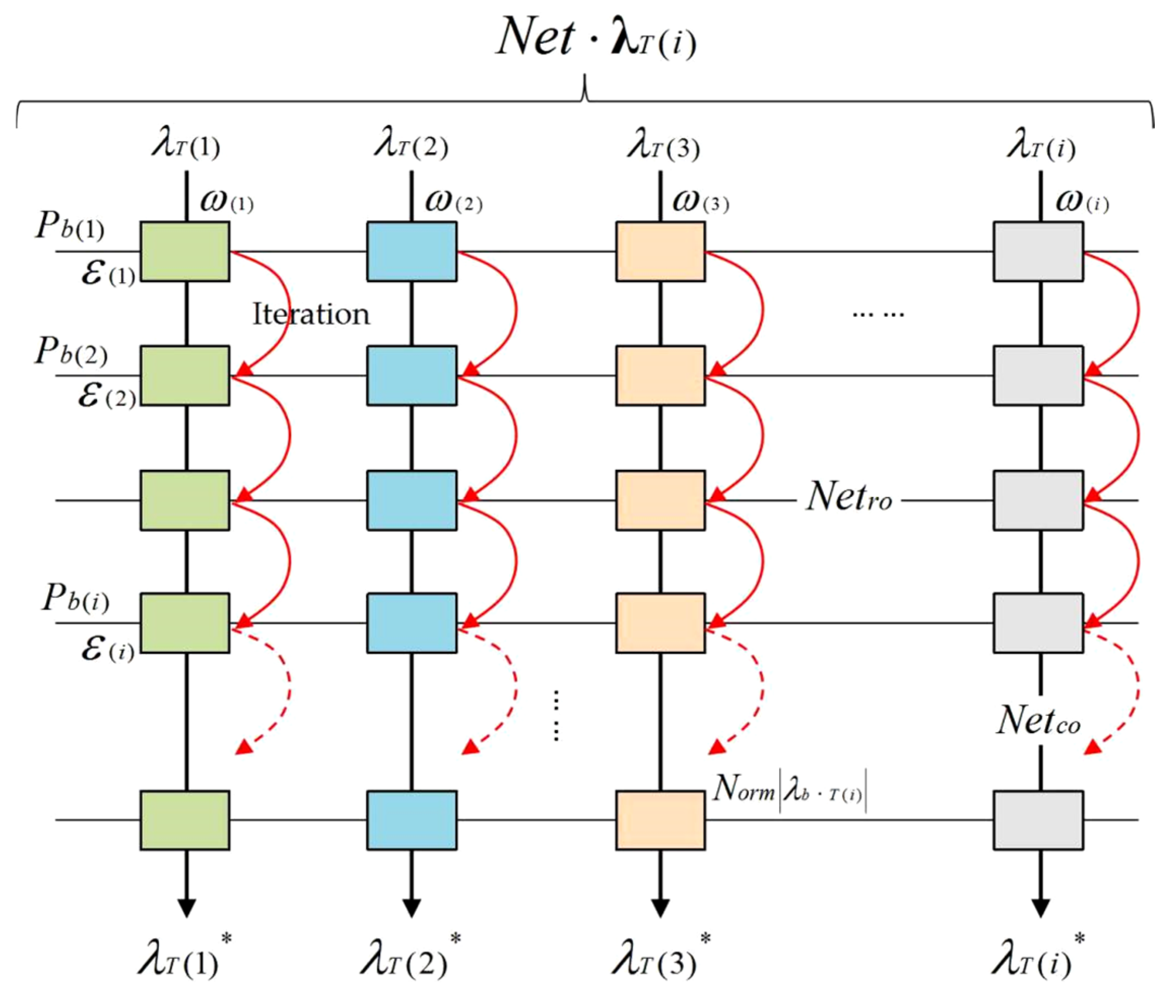
3.2.2. Improved POI Recommendation Degree Model Based on Tourism Attribute Interest Network

The Naive Bayes classification algorithm calculates the conditional probabilities of the $m$ number of destination POIs in a set $\left\{P_{a(i)}\right\}$ from the perspective of the probability that the once-visited POIs belong to different interest clusters $C_{(i)}$, and uses it as the recommendation degree ${\delta }_{NB}$. The modeling conditions of the Naive Bayes classification algorithm require that each tourism attribute ${\lambda }_{T(i)}$ be independent of the others. The proposed Naive Bayes classification algorithm uses tourism attributes such as “travel cost”, “travel time”, “POI A-Class”, and “POI popularity”. Each attribute is independent in terms of functional properties, while there is correlation in the subjective evaluation and selection of different tourists, and it will have an impact on the final recommendation of destination POIs in the set $\left\{P_{a(i)}\right\}$. Tourists have different attitudes and judgments in the evaluation correlations and interest weights of POI tourism attributes when choosing POIs for sightseeing; that is, their demand tendencies for different tourism attributes are different. To make the recommendation results output by the Naive Bayes classification algorithm more accurate, we introduce the model of tourism attribute interest weight, construct a tourism attribute interest network based on historical visited POIs, and introduce it into the conditional probability model output by the Naive Bayes classification algorithm to further optimize the POIs that accurately match tourists’ interests.

Definition 10.

Once-visited POI interest weight ${\epsilon }_{(i)}$ and tourism attribute interest weight ${\omega }_{(i)}$. Tourists evaluate and set weights for $n$ number of POIs in the once-visit POI set $\left\{P_{b(i)}\right\}$ based on their own interests. We define this weight as the once-visited POI interest weight ${\epsilon }_{(i)}$, $0<{\epsilon }_{(i)}<1$, ${\epsilon }_{(i)}\in R$. Tourists evaluate POI tourism attributes based on their own interests and set interest weights. This weight is defined as the tourism attribute interest weight ${\omega }_{(i)}$, $0<{\omega }_{(i)}<1$, ${\omega }_{(i)}\in R$. The interest weight of a tourism attribute determines the degree to which tourists attach importance to tourism attributes. The higher the weight ${\omega }_{(i)}$ is, the higher the tourist’s interest tendency towards attribute ${\lambda }_{T(i)}$ will be, and vice versa. According to the definition, the relationship model among tourism attributes is constructed from the perspective of interest weight, as shown in Formula (15), $g$ is the number of tourism attributes ${\lambda }_{T(i)}$.

$${\displaystyle \sum _{i=1}^g{\omega }_{(i)}}=1$$

(15)

Definition 11.

Tourism attribute interest network $Net·{\lambda }_{T(i)}$. The network composed of $n$ number of POIs in the POI set $\left\{P_{b(i)}\right\}$ and their tourism attribute quantification values is defined as the tourism attribute interest network, denoted as $Net·{\lambda }_{T(i)}$. The final interests of tourists in various tourism attributes are determined by the network $Net·{\lambda }_{T(i)}$. Figure 3 shows the constructed tourism attribute interest network $Net·{\lambda }_{T(i)}$. In the network, the horizontal network ${Net}_{ro}$ represents the quantified values of tourism attributes for POIs $P_{b(i)}$, while the vertical network ${Net}_{co}$ represents the iteration of each POI by the quantified values of a single tourism attribute.

According to Definitions 10 and 11, and the tourism attribute interest network $Net·{\lambda }_{T(i)}$, the tourism attribute interest iterative model ${{\lambda }_{T(i)}}^{*}$ is constructed by introducing weight ${\epsilon }_{(i)}$ and weight ${\omega }_{(i)}$, as shown in Formula (16), and $N_{orm}\left|·\right|$ represents the normalization function, $g$ represents the number of tourism attributes ${\lambda }_{T(i)}$, and $n$ represents the number of once-visited POIs $P_{b(i)}$.

$${{\lambda }_{T(i)}}^{*}=\frac{{\displaystyle \sum _{i=1}^g{\displaystyle \sum _{j=1}^n{\epsilon }_{(j)}·\left({\omega }_{(i)}·N_{orm}\left|{\lambda }_{b·T(i)}\right|\right)}}}{n}$$

(16)

According to the quantified values ${\lambda }_{a·T(i)}$ of tourism attributes in the destination POIs $P_{a(i)}$, the tourist interest matching recommendation degree ${\delta }_{MA}$ is constructed as shown in Formula (17). Due to the introduction of weight ${\epsilon }_{(i)}$ and weight ${\omega }_{(i)}$, the coefficient value $\zeta$ of the recommendation degree ${\delta }_{MA}$ is set as $\zeta =0.1$.

$${\delta }_{MA}=1-{\left[{\displaystyle \sum _{i=1}^g{\left({{\lambda }_{T(i)}}^{*}-\zeta ·N_{orm}\left|{\lambda }_{a·T(i)}\right|\right)}^p}\right]}^{\frac{1}{p}}$$

(17)

To optimize the accuracy of the Naive Bayes classification algorithm in recommending POIs, the tourist interest matching recommendation degree ${\delta }_{MA}$ is introduced into Formula (14) recommendation degree ${\delta }_{NB}=\max P(P_{a(i)}|C_{(i)})P(C_{(i)})$, and the destination POI $P_{a(i)}$ recommendation model ${\delta }_{(i)}$ is constructed as shown in Formula (18).

$${\delta }_{(i)}={\delta }_{NB} \times {\delta }_{MA}$$

(18)

The destination POI $P_{a(i)}$ recommendation model ${\delta }_{(i)}$ introduces a tourist interest weight and tourism attribute interest network based on an improved Naive Bayes classification algorithm, and the output POIs will be closer to the tourists’ interests.

3.2.3. POI Recommendation Model Based on the Spatial Decision Forest Algorithm

The structural tree $\mathrm{Tree} G_{N(i)}$ generated by the text mining algorithm is used to classify the natural attributes of the destination POIs. At the same time, based on the tourism attributes of the once-visited POIs and considering the factors in tourism planning, a symmetry-based Naive Bayes classification algorithm is constructed to classify the tourism attributes of the destination POIs. The degrees of tourists’ preferences for POIs come from the judgment on the natural attributes and tourism attributes of the once-visited POIs, that is, the comprehensive consideration of POI categories such as “natural scenery”, “cultural history”, “leisure shopping”, “amusement parks and venues”, as well as indicators such as “travel cost”, “travel time”, “POI- A Class, and “POI popularity”. When tourists judge the POI as “Most Favorite”, it indicates that they have a high level of interest in the natural attributes and tourism attributes of the POI [17]. The goal of recommending POIs and tour routes for tourists is to search for $d$ number of POIs with the highest tourist interests among the $m$ number of POIs and construct a route search algorithm to output the route with the lowest travel cost. Based on the modeling objectives, relevant definitions are provided as follows:

Definition 12. 

Recommendation decision matrix $T_{d(i)}$. Based on the natural attribute classification results output by the text mining algorithm and the tourism attribute classification results output by the Naive Bayes algorithm, a global optimal search algorithm is constructed to list the destination POIs $P_{a(i)}$ in the classification $C_{(i)}$ by the natural attributes and their recommendation degree ${\delta }_{(i, j)}$, $0<i\le k$, $0<j\le h_{(i)}$ and store them in a certain data structure in a $k\times h_{(i)}$ dimension matrix. This matrix is defined as a recommendation decision matrix, denoted as $T_{d(i)}$. The matrix consists of $k$ number of rows and $h_{(i)}$ number of columns. $k$ represents the number of natural attribute classifications and $h_{(i)}$ represents the number of destination POIs included in the tourism attribute classification $C_{(i)}$. An arbitrary row of the matrix represents a natural attribute classification $G_{N(i)}$ in the tourism attribute classification $C_{(i)}$. The matrix $T_{d(i)}$ code $i$ corresponds to the encoding of the tourism attribute classification $C_{(i)}$, that is, one classification $C_{(i)}$ corresponds to one matrix $T_{d(i)}$, $0<i\le w$, $i,w\in N$, $w$ is the number of classification $C_{(i)}$. Formula (19) is the constructed recommendation decision matrix for the classification $C_{(i)}$.

$$T_{d(i)}=\left[\begin{array}{cccc}{\delta }_{(1, 1)}& {\delta }_{(1, 2)}& \dots & {\delta }_{(1, h(i))}\\ {\delta }_{(2, 1)}& {\delta }_{(2, 2)}& \dots & {\delta }_{(2, h(i))}\\ \dots & \dots & \dots & \dots \\ {\delta }_{(k, 1)}& {\delta }_{(k, 2)}& \dots & {\delta }_{(k, h(i))}\end{array}\right]$$

(19)

Definition 13. 

Recommendation decision tree $\mathrm{Tree} C_{(i)}$ and recommendation decision forest ${Forest C}_{(i)}$. In the process of constructing a recommendation decision matrix $T_{d(i)}$ for classification $C_{(i)}$ by using the global optimal search algorithm, the destination POIs $P_{a(i)}$ and recommendation degrees ${\delta }_{(i, j)}$ are grown from the child nodes “$G_{N(i)}$” assigned by the root node “$C_{(i)}$”, and the binary tree structure is extended to the lower level. The improved binary tree derived from the matrix $T_{d(i)}$ is defined as the recommendation decision tree, denoted as $\mathrm{Tree} C_{(i)}$. A decision forest composed of a $w$ number of decision trees $\mathrm{Tree} C_{(i)}$ corresponding to classifications $C_{(i)}$ is defined as a recommendation decision forest, denoted as ${Forest C}_{(i)}$. Decision trees and decision forest are the visual representations of constructing an optimal destination POI recommendation algorithm. The decision tree $\mathrm{Tree} C_{(i)}$ meets the following conditions:

(1)

The root node represents the classification $C_{(i)}$, and the growth node represents the classification$G_{N(i)}$;

(2)

The recommendation degree ${\delta }_{(i, j)}$ of any child node$\forall N_{ode(x, y)}$ in the previous layer must be higher than that of any child node $N_{ode(x+1, \forall y)}$ in the next layer, which  $x$  represents the layer of the decision tree and  $y$  represents the node within the layer;

(3)

In the same layer, the recommendation degree${\delta }_{(i, j)}$  of the left child node$N_{ode(x, y)}$  must be higher than that of the right child node$N_{ode(x, y + \Delta )}$;

(4)

The total number of nodes in the decision tree is $k + h_{(i)} + 1$, and the total number of layers is satisfied $⌊{\log }_2(k+h_{(i)}+1)⌋$.

According to the modeling principle and Definitions 12 and 13, construct the POI recommendation model based on the spatial decision forest algorithm in Algorithm 1. Figure 4 shows the process for constructing the decision tree $\mathrm{Tree} C_{(i)}$ and decision forest ${Forest C}_{(i)}$.

Algorithm 1: The POI recommendation model based on the spatial decision forest algorithm

1: Take $i=1,$ construct a recommendation decision tree $\mathrm{Tree}{C}_{(1)}$ for tourism attribute classification $C_{(1)}$. Collect all destination POIs $P_{a(i)}$ included in $C_{(1)}$ and determine the natural attribute classification $G_{N(t)}$ that each POI belongs to. The tourism attribute classification $C_{(1)}$ includes $h_{(1)}$ number of POIs, and suppose that each natural attribute classification $G_{N(t)}$ includes $h_{(1,t)}$ number of POIs. 2: The root node is defined as $C_{(1)}$, and the growth child node is defined as $G_{N(t)}$, $0<t\le k$, $t,k\in \mathbf{N}$. Calculate the recommendation degree $\delta$ of the destination POIs $P_{a(i)}$ in $C_{(1)}$. Randomly store the POI recommendation degrees $\delta$ of each corresponding classification $G_{N(i)}$ for each row of the recommendation decision matrix $T_{d(i)}$ according to the element storage rules, denoted as ${\delta }_{(i,j)}$. 3: For growth nodes $G_{N(t)}$. Take $t=1$, which contains $h_{(1,1)}$ number of POIs, corresponding to the first row of the matrix $T_{d(i)}$. Thus, the binary tree derived from the growth node $G_{N(t)}$ contains $h_{(1,1)}$ number of child nodes. 4: Take all the elements ${\delta }_{(1,x)}$ of the first row in the matrix $T_{d(i)}$, $0<x\le h_{(1,1)}$, and derive the binary tree relating to $G_{N(1)}$. Figure 4A shows the initial state of the root node $C_{(1)}$ and the growth child node $G_{N(t)}$. 5: Judge ${\delta }_{(1,1)}$ and ${\delta }_{(1,2)}$: 6:   If ${\delta }_{(1,1)}\ge {\delta }_{(1,2)}$, store ${\delta }_{(1,1)}$ and ${\delta }_{(1,2)}$ into $N_{ode(1,1)}$ and $N_{ode(1,2)}$; 7:   If ${\delta }_{(1,1)}<{\delta }_{(1,2)}$, store ${\delta }_{(1,1)}$ and ${\delta }_{(1,2)}$ into $N_{ode(1,2)}$ and $N_{ode(1,1)}$. 8: Add ${\delta }_{(1,3)}$, compare ${\delta }_{(1,1)}$, ${\delta }_{(1,2)}$ and ${\delta }_{(1,3)}$: 9:   If ${\delta }_{(1,1)}\ge {\delta }_{(1,2)}$: 10:     If ${\delta }_{(1,1)}\ge {\delta }_{(1,2)}>{\delta }_{(1,3)}$: store ${\delta }_{(1,1)}$, ${\delta }_{(1,2)}$ and ${\delta }_{(1,3)}$ into $N_{ode(1,1)}$,      $N_{ode(1,2)}$ and $N_{ode(2,1)}$; 11:     If ${\delta }_{(1,1)}\ge {\delta }_{(1,3)}>{\delta }_{(1,2)}$: store ${\delta }_{(1,1)}$, ${\delta }_{(1,2)}$ and ${\delta }_{(1,3)}$ into $N_{ode(1,1)}$,       $N_{ode(2,1)}$ and $N_{ode(1,2)}$; 12:     If ${\delta }_{(1,3)}\ge {\delta }_{(1,1)}>{\delta }_{(1,2)}$: store ${\delta }_{(1,1)}$, ${\delta }_{(1,2)}$ and ${\delta }_{(1,3)}$ into $N_{ode(1,2)}$,      $N_{ode(2,1)}$ and $N_{ode(1,1)}$. 13:   If ${\delta }_{(1,1)}<{\delta }_{(1,2)}$: 14:     If ${\delta }_{(1,3)}<{\delta }_{(1,1)}<{\delta }_{(1,2)}$: store ${\delta }_{(1,1)}$, ${\delta }_{(1,2)}$ and ${\delta }_{(1,3)}$ into $N_{ode(1,2)}$,      $N_{ode(1,1)}$ and $N_{ode(2,1)}$; 15:     If ${\delta }_{(1,1)}<{\delta }_{(1,3)}<{\delta }_{(1,2)}$: store ${\delta }_{(1,1)}$, ${\delta }_{(1,2)}$ and ${\delta }_{(1,3)}$ into $N_{ode(2,1)}$,      $N_{ode(1,1)}$ and $N_{ode(1,2)}$; 16:     If ${\delta }_{(1,1)}<{\delta }_{(1,2)}<{\delta }_{(1,3)}$: store ${\delta }_{(1,1)}$, ${\delta }_{(1,2)}$ and ${\delta }_{(1,3)}$ into $N_{ode(2,1)}$,      $N_{ode(1,2)}$ and $N_{ode(1,1)}$. 17: Add ${\delta }_{(1,i)}$, compare ${\delta }_{(1,1)}$$~{\delta }_{(1,i)}$ in line with the same algorithm in step 5 to step 16, and store POI recommendation degrees ${\delta }_{(i,j)}$ by the binary tree descending sub-node storage rules. 18: Traverse the $h_{(1,1)}$ number of recommendation degrees ${\delta }_{(1,i)}$$~i\in (0,h_{(1,1)}]$ of child nodes until a binary tree containing $h_{(1,1)}$ number of child nodes is derived. The binary tree search algorithm for $G_{N(1)}$ ends, and a complete binary tree is generated, as shown in Figure 4B. 19: Repeat the algorithm from step 3 to step 18, searching for the binary trees derived from other classifications $G_{N(t)}$, traversing $G_{N(t)}$$~t\in (0,k]$, with each binary tree $G_{N(t)}$ containing $h_{(1,t)}$ number of child nodes. When $t=k$, the traversal process is completed, a recommendation structure tree $\mathrm{Tree}{C}_{(1)}$ consisting of $k$ number of derived binary trees from $k$ number of $G_{N(t)}$ is generated, as shown in Figure 4C. 20: Repeat steps 1 through 19. For $C_{(i)}$, take $i=2$, generate the recommendation structure tree $\mathrm{Tree}{C}_{(2)}$ for $C_{(2)}$. In the same method, traverse $C_{(i)}$$~i\in (0,w]$ and generate $w$ number of recommendation structure trees $\mathrm{Tree}{C}_{(i)}$. 21: Generate a recommendation decision forest $Forest{C}_{(i)}$ by $w$ number of recommendation decision trees $\mathrm{Tree}{C}_{(i)}$, as Figure 4D shows. In the decision forest, the sub-node $N_{ode(1,1)}$ of $G_{N(t)}$ in each $\mathrm{Tree}{C}_{(i)}$ store has the highest recommendation degree, and its related destination POI $P_{a(i)}$ is the optimal POI for $G_{N(t)}$. The algorithm recommends the optimal POIs $G_{N(t)}$ as the tour route POIs, representing the natural attributes and tourism attributes with the highest tourist interests.

3.3. POI Tour Route Recommendation Model Based on the Spatial Decision Tree Algorithm

By using the POI recommendation model, the decision trees $\mathrm{Tree} C_{(i)}$ and decision forest $Forest C_{(i)}$ representing the tourism attribute classifications $C_{(i)}$ are obtained. The optimal POI recommendation is realized by selecting the sub-nodes with the best recommendation degrees $\delta$ from the natural attribute classifications $G_{N(t)}$ included in the decision tree. From a geospatial perspective, POIs are distributed in different geographical locations of tourism cities and have spatial attributes. Their spatial accessibility is constrained by various factors, such as geographical coordinates, road distances, accessibility time, and transportation tools. Therefore, constructing a tour route model based on the recommended POIs is an effective way to obtain the optimal travel route [18,19,20]. We integrate the urban geospatial constraints and construct a POI tour route recommendation model based on the spatial decision tree algorithm. The relevant definitions are given as follows:

Definition 14. 

Tour route vector $T_{ro}$ and vector element $T_{ro(i)}$. Tourists start traveling from the starting point $S$ in the city, and the traveling process forms a complete route by following a certain sequence of $d$ number of POIs recommended by the decision forest algorithm. Extract the route as a $1\times d$ dimension vector, randomly store $d$ number of POIs into the vector, and define this vector as a tour route vector, denoted as $T_{ro}$. The elements in the vector are denoted as $T_{ro(i)}$. According to the definition, the starting point $S$ traverses the $d$ number of elements $T_{ro(i)}$ of vector $T_{ro}$ to form a POI storage order, which represents a tour route, $i ~ i\in (0,d]$, $i,d\in N$.

Definition 15. 

Route sub-interval $subin·T_{ro(i, j)}$ and route interval $in·T_{ro}$. The path interval between arbitrary adjacent elements $T_{ro(i)}$ and $T_{ro(j)}$ in vector $T_{ro}$ is defined as a route sub-interval, denoted as $subin·T_{ro(i, j)}$. The whole traveling interval composed of the POI storage vector $T_{ro}$ is defined as the route interval, denoted as $in·T_{ro}$. sub-interval $subin·T_{ro(i, j)}$ represents the moving and traveling space between POIs, while interval $in·T_{ro}$ represents the tour route.

Definition 16. 

Sub-interval cost $f_{subin·T_{ro(i, j)}}$ and interval cost $f_{in·T_{ro}}$. The distance between road nodes $n_{ode(x)}$ and $n_{ode(x + 1)}$ that form the sub-interval $subin·T_{ro(i, j)}$ is $D_{(x,x + 1)}$ (Unit: km), then the spatial cost $f_{subin·T_{ro(i, j)}}$ for tourists to move from the node $T_{ro(x)}$ to the node $T_{ro(x + 1)}$ meets the Formula (20), $k$ is the number of road nodes within the sub-interval. The spatial cost between the POI nodes $T_{ro(x)}$ and $T_{ro(x + 1)}$ that make up the tour route interval $in·T_{ro}$ is $f_{subin·T_{ro(i, j)}}$, then the spatial cost $f_{in·T_{ro(x, x + 1)}}$ generated by tourists traveling from the starting point $S$ to the last POI element $T_{ro(i)}$ of the vector $T_{ro}$ meets Formulas (21) or (22), $f_{subin·T_{ro(S, 1)}}$ represents the spatial cost between the starting point $S$ and the first POI element $T_{ro(1)}$ of the vector $T_{ro}$.

$$f_{subin·T_{ro(i, j)}}={\displaystyle \sum _{x=1}^{k}D(x,x+1)}$$

(20)

$$f_{in·T_{ro(x, x + 1)}}=f_{subin·T_{ro(S, 1)}}+{\displaystyle \sum _{x=1}^{d-1}{f}_{subin·T_{ro(i, j)(x)}}}$$

(21)

$$f_{in·T_{ro(x,x + 1)}}=f_{subin·T_{ro(S,1)}}+{\displaystyle \sum _{x=1}^{d-1}{\displaystyle \sum _{\gamma =1}^k{D}_{(\gamma ,\gamma +1)}}}$$

(22)

Definition 17. 

Sub-interval decision tree $subtr·T_{ro(i, j)}$ and interval decision tree $tr·T_{ro}$. Using the sub-interval costs $f_{subin·T_{ro(i, j)}}$ formed by multiple roads within the sub-interval $subtr·T_{ro(i, j)}$ as nodes, a cost-complete binary tree is constructed via a heap sorting algorithm, and the complete binary tree is defined as a sub-interval decision tree, denoted as $subtr·T_{ro(i, j)}$. Using the interval costs $f_{in·T_{ro}}$ formed by the $d$ number of POIs contained within the interval $in·T_{ro}$ and the starting point $S$ as nodes, a cost complete binary tree is constructed via the heap sorting algorithm, and the complete binary tree is defined as an interval decision tree, denoted as $tr·T_{ro}$. According to the characteristics of a complete binary tree, both decision trees $subtr·T_{ro(i, j)}$ and $tr·T_{ro}$ meet the following modeling conditions:

(1) 

The root node stores the minimum cost  $f_{subin·T_{ro(i, j)}}$  or  $f_{in·T_{ro}}$;

(2) 

The cost  $f_{subin·T_{ro(i, j)}}$  or  $f_{in·T_{ro}}$  of arbitrary child node in the previous layer must be smaller than the cost of arbitrary child node in the next layer;

(3) 

In the same layer, the cost  $f_{subin·T_{ro(i, j)}}$  or  $f_{in·T_{ro}}$  of the left child node must be smaller than the cost of arbitrary right child node;

(4) 

When the total number of nodes is $n$, the height of the tree’s layer meets $⌊{\log }_{2}n⌋$.

Based on Definitions 14–17 and the POI tour route modeling approach, we construct a POI tour route recommendation model based on the spatial decision tree algorithm. The POI route algorithm consists of two parts: Algorithm 2 is to find out the optimal solution of the route sub-interval $subin·T_{ro(i, j)}$, and Algorithm 3 is to find out the optimal solution of the route interval $in·T_{ro}$.

Algorithm 2: Optimal solution algorithm of the route sub-interval $subin·T_{ro(i,j)}$

1: Establish a vector $T_{ro}$ and confirm the vector elements $T_{ro(i)}$. Establish a sub-interval $subin·T_{ro(i,j)}$ containing elements $T_{ro(i)}$, $T_{ro(j)}$ and $k$ number of road nodes $n_{ode(x)}$. Figure 5A shows an example process for constructing the sub-interval $subin·T_{ro(i,j)}$. 2: Randomly search for the moving path $Pat{h}_{(1)}$ between $T_{ro(i)}$ and $T_{ro(j)}$, and iteratively calculate the cost $f_{subin·T_{ro(i,j)}(1)}$. 3:   Connect $T_{ro(i)}$ and $n_{ode}(1)$, there is no closed loop; the moving path distance is   $D_{(T_{ro(i)},1)}$, as shown in Figure 5B; 4:   Connect $n_{ode}(1)$ and $n_{ode}(2)$, there is no closed loop; the moving path distance   is $D_{(1,2)}$, as shown in Figure 5C; 5:   Connect $n_{ode}(2)$ and $n_{ode}(3)$, there is no closed loop; the moving path distance    is $D_{(2,3)}$, as shown in Figure 5D; 6:   Connect $n_{ode}(3)$ and $n_{ode}(1)$, there is a closed loop, delete $n_{ode}(1)$; connect $n_{ode}(5)$,   there is no closed loop, the moving path distance is $D_{(3,5)}$, as shown in Figure 5E 7:   Continue searching, connect $n_{ode}(5)$ and $n_{ode}(8)$, $n_{ode}(8)$, $T_{ro(j)}$, form a   complete moving path $Pat{h}_{(1)}$, as shown in Figure 5F. Formula (23) shows the   interval cost example of $f_{subin·T_{ro(i,j)}(1)}$. 8: Randomly search for the moving path $Pat{h}_{(2)}$ between $T_{ro(i)}$ and $T_{ro(j)}$, and iteratively calculate the cost $f_{subin·T_{ro(i,j)}(2)}$. 9: Continue the searching by using the method from step 2 to step 8. Traverse $k$ number of road nodes $n_{ode(x)}$ to form $g$ number of paths $Pat{h}_{(i)}$ without a closed loop, $i\in (0,g]$, $i,g\in N$, corresponding to $g$ number of sub-interval costs $f_{subin·T_{ro(i,j)}(i)}$. The mark $g$ relates to the $g$ number of nodes in the sub-interval decision tree $subtr·T_{ro(i,j)}$. 10: Take the costs $f_{subin·T_{ro(i,j)}(i)}$ of the $g$ number of paths $Pat{h}_{(i)}$ and construct a complete binary tree containing $g$ number of nodes. Figure 6A shows the initial state of the binary tree. 11: Judge $f_{subin·T_{ro(i,j)}(1)}~f_{subin·(1)}$ and $f_{subin·T_{ro(i,j)}(2)}~f_{subin·(2)}$: 12:   If $f_{subin·(1)}\ge f_{subin·(2)}$, store $f_{subin·(1)}$ and $f_{subin·(2)}$ into $c_{node(1,1)}$ and $f_{node}$; 13:   If $f_{subin·(1)}<f_{subin·(2)}$, store $f_{subin·(1)}$ and $f_{subin·(2)}$ into $f_{node}$ and $c_{node(1,1)}$. 14: Add $f_{subin·T_{ro(i,j)}(3)}~f_{subin·(3)}$, compare $f_{subin·(1)}$, $f_{subin·(2)}$ and $f_{subin·(3)}$: 15:   If $f_{subin·(1)}\ge f_{subin·(2)}$: 16:     If $f_{subin·(1)}\ge f_{subin·(2)}>f_{subin·(3)}$: store $f_{subin·(1)}$, $f_{subin·(2)}$ and     $f_{subin·(3)}$ into $c_{node(1,2)}$, $c_{node(1,1)}$ and $f_{node}$; 17:     If $f_{subin·(1)}\ge f_{subin·(3)}>f_{subin·(2)}$: store $f_{subin·(1)}$, $f_{subin·(2)}$ and     $f_{subin·(3)}$ into $c_{node(1,2)}$, $f_{node}$ and $c_{node(1,1)}$; 18:     If $f_{subin·(3)}\ge f_{subin·(1)}>f_{subin·(2)}$: store $f_{subin·(1)}$, $f_{subin·(2)}$ and     $f_{subin·(3)}$ into $c_{node(1,1)}$, $f_{node}$ and $c_{node(1,2)}$. 19:   If $f_{subin·(1)}<f_{subin·(2)}$: 20:     If $f_{subin·(3)}<f_{subin·(1)}<f_{subin·(2)}$: store $f_{subin·(1)}$, $f_{subin·(2)}$ and     $f_{subin·(3)}$$\mathrm{into}{c}_{node(1,1)}$, $c_{node(1,2)}$, and $f_{node}$; 21:     If $f_{subin·(1)}<f_{subin·(3)}<f_{subin·(2)}$: store $f_{subin·(1)}$, $f_{subin·(2)}$ and     $f_{subin·(3)}$ into $f_{node}$, $c_{node(1,2)}$ and $c_{node(1,1)}$; 22:     If $f_{subin·(1)}<f_{subin·(2)}<f_{subin·(3)}$: store $f_{subin·(1)}$, $f_{subin·(2)}$ and     $f_{subin·(3)}$ into $f_{node}$, $c_{node(1,1)}$ and $c_{node(1,2)}$. 23: Add $f_{subin·T_{ro(i,j)}(i)}~f_{subin·(i)}$, compare $f_{subin·(1)}$$\text{~}{f}_{subin·(i)}$ by the same algorithm from the step 11 to step 22, and store $f_{subin·(i)}$ in a binary tree by an ascending heap sorting algorithm. After traversing the sub-nodes $i=g$, the cost $f_{subin·(i)}$ algorithm ends, and the binary tree is output as shown in Figure 6B. 24: The sub-interval cost $f_{subin·T_{ro(i,j)}(i)}$ stored by the root node $f_{node}$ of the current binary tree represents the minimum cost, and the corresponding path $Pat{h}_{(i)}$ is the optimal path between $T_{ro(i)}$ and $T_{ro(j)}$. 25: In line with the method from step 1 to step 24, traverse to search for all the optimal solutions in sub-intervals $subin·T_{ro(i,j)}$. The algorithm ends.

$$f_{subin·T_{ro(i, j)}(1)}=D_{(T_{ro(i)}, 1)}+D_{(1, 2)}+D_{(2, 3)}+D_{(3, 5)}+D_{(5,8)}+D_{(8, T_{ro(j)})}$$

(23)

Figure 5. The example modeling process of constructing the sub-interval $subin·T_{ro(i, j)}$. (A) shows the initial status of the sub-interval. (B) shows the node $n_{ode}(1)$ has been found. (C) shows the node $n_{ode}(2)$ has been found. (D) shows the node $n_{ode}(3)$ has been found. (E) shows the node $n_{ode}(5)$ has been found. (F) shows the node $n_{ode}(8)$ has been found, and finally the path has been found.

Figure 5. The example modeling process of constructing the sub-interval $subin·T_{ro(i, j)}$. (A) shows the initial status of the sub-interval. (B) shows the node $n_{ode}(1)$ has been found. (C) shows the node $n_{ode}(2)$ has been found. (D) shows the node $n_{ode}(3)$ has been found. (E) shows the node $n_{ode}(5)$ has been found. (F) shows the node $n_{ode}(8)$ has been found, and finally the path has been found.

Figure 6. The constructed complete binary tree $subtr·T_{ro(i, j)}$ when searching for the optimal solution in the sub-interval $subin·T_{ro(i, j)}$. (A) shows the initial state of the binary tree. (B) shows the output binary tree.

Figure 6. The constructed complete binary tree $subtr·T_{ro(i, j)}$ when searching for the optimal solution in the sub-interval $subin·T_{ro(i, j)}$. (A) shows the initial state of the binary tree. (B) shows the output binary tree.

Algorithm 3: The $tr·T_{ro}$ algorithm to find out the optimal solution for interval $in·T_{ro}$.

1: Establish a vector $T_{ro}$ and confirm the vector elements $T_{ro}(i)$. Establish a route interval $in·T_{ro}$, containing the $d$ number of recommended POIs. 2: Construct the first tour route ${Tour}_{(1)}$, relating to the interval cost $f_{in·T_{ro}}$. Randomly store the $d$ number of POIs to $T_{ro}$, output the optimal sub-interval cost $f_{subin·T_{ro}(S,1)}$ between the starting point $S$ and the current $T_{ro(1)}$, and the optimal sub-interval cost $f_{subin·T_{ro(i,j)}}$ between arbitrary element $\forall T_{ro(x)}$ and its adjacent element $\forall T_{ro(x+1)}$. 3: Bring costs into Formulas (21) or (22) of the interval cost model $f_{in·T_{ro(x,x+1)}}$ to calculate the interval cost $f_{in·T_{ro(x,x+1)(1)}}$ of the route ${Tour}_{(1)}$. 4: Based on the vector $T_{ro}$ containing $d$ number of POI elements $T_{ro(i)}$, according to the tour sequence, randomly exchange the storage element$T_{ro(i)}$ and output $A_{(d,d)}$ kinds of routes ${Tour}_{(i)}$$,i\in (0,A_{(d,d)}]$$,i,A_{(d,d)}\subset N$. Traverse $A_{(d,d)})$ kinds of routes ${Tour}_{(i)}$ and output the route costs $f_{in·T_{ro(x,x+1)(i)}}~f_{in·(i)}$. 5: Use the heap-ascending algorithm to store interval costs $f_{in·T_{ro(x,x+1)(i)}}~f_{in·(i)}$ into a complete binary tree, constructing a complete binary tree containing $A_{(d,d)}$ number of nodes. Figure 7A shows the initial state of the binary tree, and Figure 7B shows the constructed heap-ascending complete binary tree. 6: Traverse $i~(0,A_{(d,d)}]$, when the sub-node $i=A_{(d,d)}$ has been iterated, the interval $in·T_{ro}$ search algorithm ends. The current binary tree root node $f_{node}$ stores the minimum interval cost $f_{in·T_{ro(x,x+1)(i)}}$, and the corresponding route ${Tour}_{(i)}$ is the route with the lowest cost from the starting point $S$ to travel through the $d$ number of recommended POIs.

Figure 7. The constructed complete binary tree $tr·T_{ro}$ when searching for the optimal solution in the interval $in·T_{ro}$. (A) shows the initial state of the binary tree. (B) shows the output binary tree.

Figure 7. The constructed complete binary tree $tr·T_{ro}$ when searching for the optimal solution in the interval $in·T_{ro}$. (A) shows the initial state of the binary tree. (B) shows the output binary tree.

3.4. The Construction of Tourist Satisfaction Evaluation Model

To verify the feasibility of the proposed POI route recommendation algorithm and the effectiveness of the tourist feedback satisfaction based on the recommendation results, we construct tourist satisfaction evaluation models for the recommended POIs and the searched routes based on the evaluation criteria of the POI and tour route recommendation. The models evaluate the proposed POI route recommendation algorithm and the comparative methods in terms of four satisfaction indexes: average precision, average recall, average deviation of attribute matching degree, and average deviation of route cost. The satisfaction evaluation models and evaluation methods are constructed as follows:

Table 1. Tourist satisfaction evaluation indexes for POI and route recommendation.

	Average Precision	Average Recall	Average Deviation of Attribute Matching Degree	Average Deviation of Route Cost
POI recommendation	√	√	√
Route recommendation	√	√		√

shows the tourist satisfaction evaluation indexes for POI and route recommendation; the mark “√” represents the index that is used to evaluate the related item.

(1)

Average precision and average recall for POI recommendation

Set one tourist sample as $X_{(i)}$, and the interest data provided by the tourist sample are: ① historical visited POIs $P_{b(i)}$; ② the expected natural attributes $G_{N(i)}$ of POIs; ③ the number of expected POIs to visit. The algorithm recommends a $N_{POI}$ number of destination POIs $P_{a(i)}$ based on the constraints provided by the tourist sample while outputting the natural attributes $G_{N(i)}$, of tourism, such as “travel cost”, “travel time”, “POI A-Class”, “POI popularity”, and a detailed introduction to POIs for the tourist sample. The tourist sample makes a “satisfactory” (S) and “unsatisfactory” (NS) judgment on the $N_{POI}$ number of recommended POIs $P_{a(i)}$. For the $N_{POI}$ number of recommended POIs, we set the number of POIs that make the tourist make a ‘dissatisfied’ (NS) judgment is $N_{POI(i)}$, and the number of POIs that make a ‘satisfied’ (S) judgment is $N-N_{POI(i)}$. If the number of tourist samples participating in the satisfaction evaluation is $k$, the average precision evaluation model of the POI recommendation algorithm based on tourist sample $X_{(i)}$ is constructed as Formula (24). If the number of the total destination POIs $P_{a(i)}$ is $m$, and all POI samples $P_{a(i)}$ have been browsed by tourists, then the average recall evaluation model of the POI recommendation algorithm for the tourist sample is constructed as Formula (25). The $k$ number of samples in the model can also represent $k$ types or pieces of interest.

The average precision reflects the proportion of satisfied POIs selected from the recommended POIs by the overall sample of tourists to all the recommended POIs. The higher the average precision is, the higher the satisfaction of tourists with the recommended POIs will be, indicating that the precision of the recommendation algorithm is higher, and vice versa. The average recall reflects the proportion of the satisfied POIs selected from the recommended POIs by the overall sample of tourists to the total destination POIs in the research domain. The higher the average recall is, the higher the satisfaction of tourists will be, and the higher the precision of the algorithm in recommending satisfied POIs from all POIs will be.

$${\overline{P}}_{recision}=\frac{1}{k}\times {\displaystyle \sum _{i=1}^k\frac{N_{POI}-N_{POI(i)}}{N_{POI}}}$$

(24)

$${\overline{R}}_{ecall}=\frac{1}{k}\times {\displaystyle \sum _{i=1}^k\frac{N_{POI}-N_{POI(i)}}{m}}$$

(25)

(2)

Average precision and average recall of POI route

Set one tourist sample as $X_{(i)}$. Based on the $N_{POI}$ number of recommended POIs, the POI route algorithm searches for the optimal tour routes and recommends them to the tourist sample. When the recommended number of POIs is $N_{POI}$, the overall sample number of tour routes that meet the algorithm conditions is $A(N_{POI},N_{POI})$, and the optimal number of tour routes recommended by the algorithm for tourist sample under this condition is $N_{Route}$. At the same time, the system introduces information such as the direction, tendency, itinerary, and travel cost of each recommended route to the tourist, and the tourist sample makes “satisfied” (S) and “dissatisfied” (NS) judgments on the recommended routes. For the $N_{Route}$ number of recommended routes, the number of POIs that make the sample tourist make a “dissatisfied” (NS) judgment is $N_{Route(i)}$, and the number of POIs that make a “satisfied” (S) judgment is $N_{route}-N_{route(i)}$. If the number of tourist samples participating in the satisfaction evaluation is $k$, the average precision evaluation model of the POI route algorithm is constructed based on the tourist sample $X_{(i)}$ as shown in Formula (26). If tourists have browsed all the routes, the average recall evaluation model of the POI route recommendation algorithm is constructed based on the tourist sample $X_{(i)}$, as shown in Formula (27). The $k$ number of samples in the model can also represent $k$ types or pieces of interest.

The average precision reflects the proportion of satisfied routes selected from the recommended routes by the overall sample of tourists for all the recommended routes. The higher the average precision, the higher the satisfaction of tourists with the recommended routes will be. It indicates that the accuracy of the recommended routes by the recommendation algorithm is higher, and vice versa. The average recall reflects the proportion of satisfied routes selected from the recommended routes by the overall sample of tourists among all the feasible routes in the research domain. The higher the average recall is, the higher the satisfaction of tourists will be, and the higher the accuracy of the algorithm in recommending satisfied routes from all the feasible routes will be.

$${\overline{P}}_{recision}=\frac{1}{k}\times {\displaystyle \sum _{i=1}^k\frac{N_{Route}-N_{Route(i)}}{N_{Route}}}$$

(26)

$${\overline{R}}_{ecall}=\frac{1}{k}\times {\displaystyle \sum _{i=1}^k\frac{N_{Route}-N_{Route(i)}}{A(N_{POI},N_{POI})}}$$

(27)

(3)

The average deviation of attribute matching degree

As to the “satisfied” (S) and “dissatisfied” (NS) judgments on the recommended POIs made by the sample tourist $X_{(i)}$, among which the $N-N_{POI(i)}$ number of “satisfied” POIs completely conforms to the tourist’s interests, while the $N_{POI(i)}$ number of “dissatisfied” POIs does not conform to the tourist’s interests. For the dissatisfied POIs, the tourist selects other $N_{POI(i)}$ number of satisfied POIs to replace. Note the POI sample recommended by the algorithm but marked “dissatisfied” as $P_{NS(u)}$, with its tourism attribute recorded as ${\lambda }_{TNS(i, j)}$. The POI that is replaced by the tourist sample is noted as $P_{Sel(u)}$, and its tourism attribute is recorded as ${\lambda }_{TSel(i, j)}$. The mark $i$ represents the POI number and $j$ represents the tourism attribute number. Then the POI deviation model of attribute matching degree for one tourist sample $X_{(i)}$ is constructed in Formula (28), $g$ is the number of tourism attributes. The average deviation model of attribute matching degree is shown in Formula (29).

The average deviation of attribute matching degree represents the spatial distance between the tourist’s satisfied POI and the recommended dissatisfied POI. The smaller the average deviation is, the higher the matching degree between the POI tourism attributes recommended by the algorithm and the tourist’s interests will be, and the stronger the algorithm’s ability to meet the tourist’s interests will be, and vice versa.

$$D_{ev\mathrm{POI}\left(u\right)}={\displaystyle \sum _{i=1}^{N_{POI(u)}}{\left({\displaystyle \sum _{j=1}^g{\left|{\lambda }_{TNS(i,j)}-{\lambda }_{TSel(i,j)}\right|}^p}\right)}^{\frac{1}{p}}}$$

(28)

$${\overline{D}}_{ev\mathrm{POI}}=\frac{1}{k}\times {\displaystyle \sum _{u=1}^k{D}_{ev\mathrm{POI}(u)}}$$

(29)

(4)

Average deviation of route cost

For the “satisfied” (S) and “dissatisfied” (NS) judgments on the recommended routes, the $N_{route}-N_{route(i)}$ number of “satisfied” routes completely conforms to the tourist’s interests, while the $N_{route(i)}$ number of “dissatisfied” routes does not conform to the tourist’s interests. For the dissatisfied routes, the tourist selects satisfied ones to replace. Set the route recommended by the algorithm but “dissatisfied” by tourist is $T_{NS(u)}$, and its travel cost is $f_{TNS(u,v)}$, note the route that replace $T_{NS(u)}$ by tourist is $T_{Sel(u)}$, and its travel cost is $f_{TSel(u,v)}$. The $u$ is the tourist number and $v$ is the route number, the deviation model of route cost for the tourist sample is constructed in Formula (30); and the average deviation of route cost is constructed in Formula (31).

The average deviation of route cost represents the overall cost difference between the routes that tourists are satisfied with and the recommended routes that they are not satisfied with. The smaller the average deviation is, the closer the recommended route cost of the algorithm to the tourists’ needs and budget will be, and the stronger the algorithm’s ability to meet tourists’ interests will be, and vice versa.

$$D_{ev\mathrm{Route}(u)}={\displaystyle \sum _{v=1}^{N_{route(u)}}\left|f_{TNS(u, v)}-f_{TSel(u, v)}\right|}$$

(30)

$${\overline{D}}_{ev\mathrm{Route}}=\frac{1}{k}\times {\displaystyle \sum _{u=1}^k{D}_{ev\mathrm{Route}(u)}}$$

(31)

4. Experiment and Results Analysis

4.1. Experimental Approach and Process

To verify the feasibility and advantages of the proposed algorithm, we designed the validation experiment and the comparative experiment. The specific experimental approaches and processes are as follows:

(1)

The first step is to use the constructed text mining algorithm to achieve destination POI natural attribute classification. Select the destination POIs of the tourism city, collect POI natural attribute labels ${\lambda }_{N(i)}$ and sub-labels ${\lambda }_{N(i, j)}$, and construct the natural attribute vector ${\lambda }_{N(i)}$ and natural attribute matrix ${\lambda }_{N(i, j)}$. By calculating the statistical label word frequency $t{f}_{({\lambda }_{N(i)})}$, inverse text frequency $id{f}_{({\lambda }_{N(i)})}$ and label weight $tfid{f}_{({\lambda }_{N(i)})}$ of each row for sub-labels in the matrix ${\lambda }_{N(i, j)}$, a natural attribute structure tree $\mathrm{Tree}{G}_{N(i)}$ of the POI is constructed to determine the natural classification of the POI.

(2)

The second step is to collect tourists’ once-visited POIs and confirm their tourism attributes and quantified intervals. Tourists determine their preferences for the tourism attributes and thus construct a training set for the Naive Bayes classification algorithm. By constructing the Naive Bayes classifier, the recommendation degrees of the destination POIs are calculated, and the tourism attribute classifications are obtained. By combining the natural attribute classification and tourism attribute classification, establish a destination POI decision tree and decision forest, and output the optimal POI recommendation.

(3)

The third step is to output sub-interval decision trees $subtr·T_{ro(i, j)}$ and an interval decision tree $tr·T_{ro}$ containing costs based on the recommended POIs and the urban geospatial constraints. Calculate the interval cost $f_{in·T_{ro}}$ of each tour route and ultimately output the optimal tour route.

(4)

The fourth step is to select the two most commonly used electronic maps for tourism route planning, GaoDe Map and 360 Map, as the control group method, while the proposed algorithm is set as the experimental group. Use the same experimental conditions and methods to output the optimal tour routes, make comparisons on the costs of the optimal routes from the three methods, and then get the relative results and conclusions.

(5)

To evaluate the satisfaction degree of sample tourists with recommended POIs and POI routes, we use the satisfaction evaluation models constructed in Section 3.4 to make comparisons between the proposed algorithm (PRA), the item-based collaborative filtering recommendation method (IBCF), and the user-based collaborative filtering recommendation method (UBCF) in terms of POI average precision, average recall, and average deviation of attribute matching degree. At the same time, make comparisons between the proposed algorithm (PRA) and the map-searching algorithms GDM and 360M in terms of average precision, average recall, and average deviation of route cost. According to the satisfaction evaluation models constructed in Section 3.4, each evaluation index could represent and reflect a tourist’s satisfaction degree.

4.2. Data Collection

The experiment collects the following data.

(1)

For the destination POI natural attribute classification, select an encyclopedia big data text containing 10,000 words, including natural attribute sub-label text. Select another 1000 texts about POI introduction as the POI text mining corpus. Divide the natural attribute category into the following labels: $G_{N(1)}$ “natural scenery”, $G_{N(2)}$ “cultural history”, $G_{N(3)}$ “leisure shopping” and $G_{N(4)}$ “amusement park and venue”. Each label contains 5 sub-labels ${\lambda }_{N(i, j)}$, and the data table is shown in Table 2. When calculating, synonyms and related words related to the sub-labels are also included in the statistics. Calculate the $tfid{f}_{({\lambda }_{N(i)})}$ for each label ${\lambda }_{N(i)}$, and construct the natural attribute structure tree of POI $\mathrm{Tree}{G}_{N(i)}$ to output its natural attribute classification $G_{N(i)}$.

The selected 15 destination POIs in the tourism city Chengdu are: $P_{a(1)}$ Jinsha Site; $P_{a(2)}$ Tazishan Park; $P_{a(3)}$ Kuanzhai Alley; $P_{a(4)}$ Jinniu Wanda; $P_{a(5)}$ Happy Valley; $P_{a(6)}$ Eastern Suburb Memory; $P_{a(7)}$ The People’s Park; $P_{a(8)}$ Raffles Plaza; $P_{a(9)}$ Sichuan Museum; $P_{a(10)}$ Du Fu Thatched Cottage; $P_{a(11)}$ San Sheng Hua Xiang; $P_{a(12)}$ Chunxi Road; $P_{a(13)}$ Guose Tianxiang Amusement Park; $P_{a(14)}$ Qinglong Lake; $P_{a(15)}$ Huanhuaxi Park.

Table 2. The collected labels and sub-labels for natural attribute classification.

$\mathbf{Label} {\mathit{\lambda }}_{\mathit{N}(\mathit{i})}$		${\mathit{\lambda }}_{\mathit{N}(1)}$ Natural Scenery	${\mathit{\lambda }}_{\mathit{N}(2)}$ Cultural History	${\mathit{\lambda }}_{\mathit{N}(3)}$ Leisure Shopping	${\mathit{\lambda }}_{\mathit{N}(4)}$ Amusement Park and Venue
Sub-label	${\lambda }_{N(i, 1)}$	River view	Historical site	Culinary experience	Leisure sports
	${\lambda }_{N(i, 2)}$	Lake and reservoir	Ancient town and city	Shopping	Sports and competitions
	${\lambda }_{N(i, 3)}$	Greenland and park	Landscape art	Theater and movie	Anime and animation
	${\lambda }_{N(i, 4)}$	Forest view	Folk culture	Indoor leisure	Adventure experience
	${\lambda }_{N(i, 5)}$	Mountain view	Royal Mausoleum	Theater performance	Rides and shows

Table 2. The collected labels and sub-labels for natural attribute classification.

$\mathbf{Label} {\mathit{\lambda }}_{\mathit{N}(\mathit{i})}$		${\mathit{\lambda }}_{\mathit{N}(1)}$ Natural Scenery	${\mathit{\lambda }}_{\mathit{N}(2)}$ Cultural History	${\mathit{\lambda }}_{\mathit{N}(3)}$ Leisure Shopping	${\mathit{\lambda }}_{\mathit{N}(4)}$ Amusement Park and Venue
Sub-label	${\lambda }_{N(i, 1)}$	River view	Historical site	Culinary experience	Leisure sports
	${\lambda }_{N(i, 2)}$	Lake and reservoir	Ancient town and city	Shopping	Sports and competitions
	${\lambda }_{N(i, 3)}$	Greenland and park	Landscape art	Theater and movie	Anime and animation
	${\lambda }_{N(i, 4)}$	Forest view	Folk culture	Indoor leisure	Adventure experience
	${\lambda }_{N(i, 5)}$	Mountain view	Royal Mausoleum	Theater performance	Rides and shows

(2)

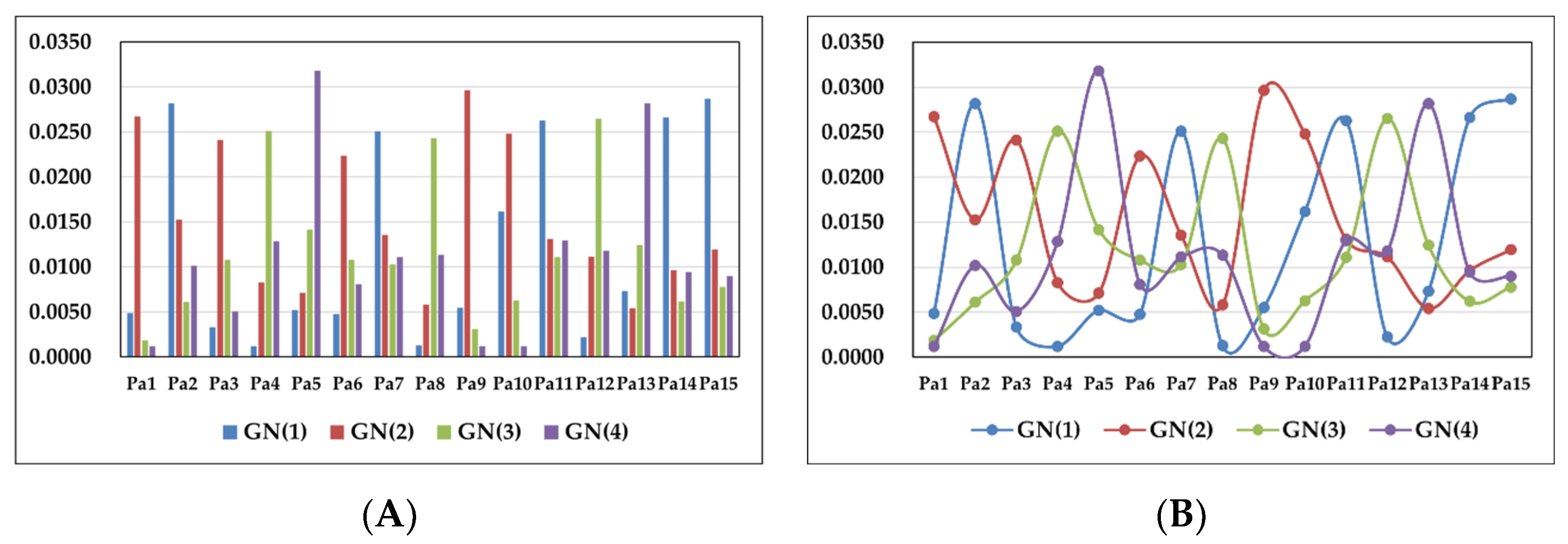
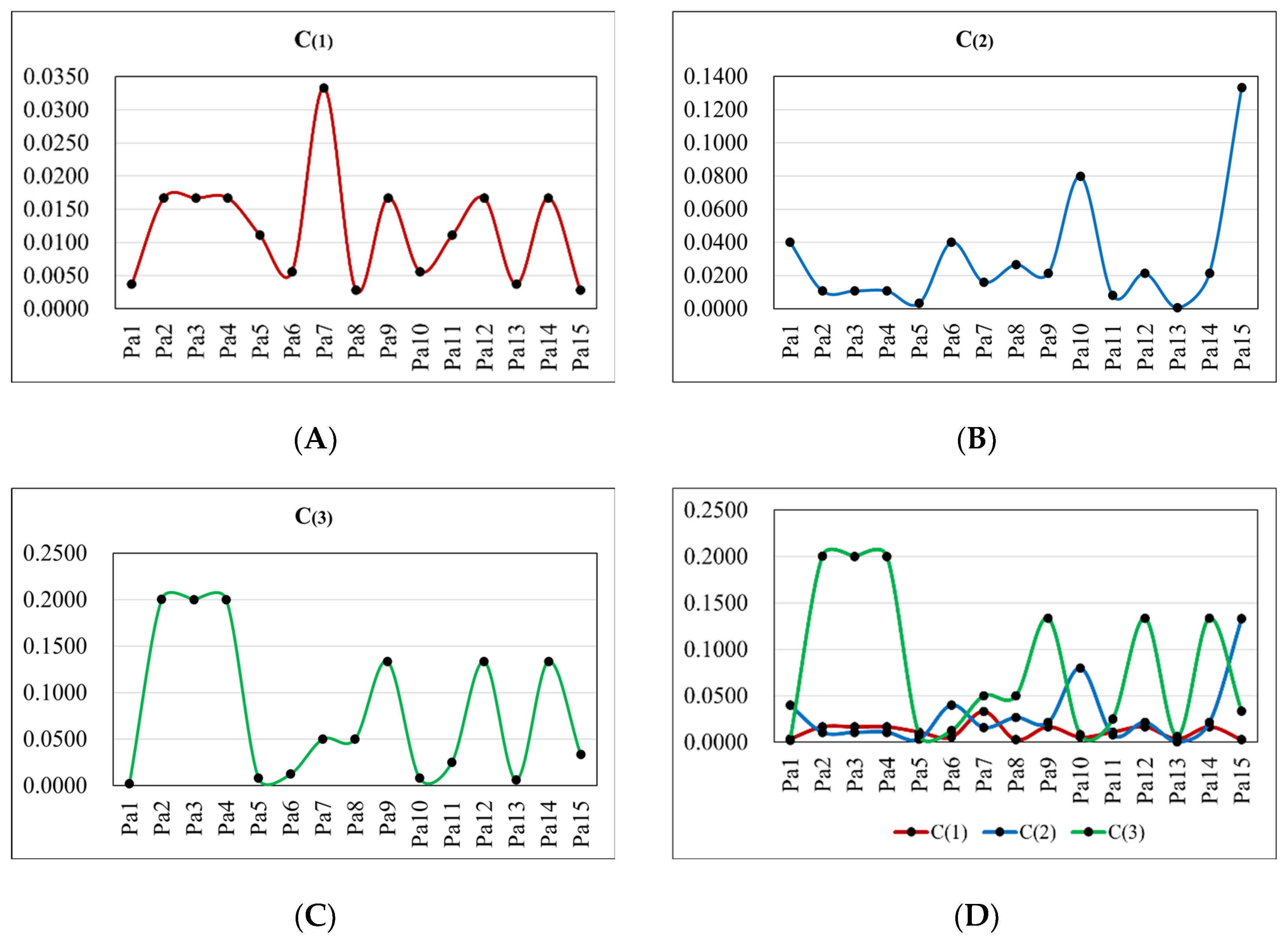
For the tourism attribute classification of destination POIs, suppose a sample tourist for the experiment. Use the tourist’s once-visited 15 POIs as well as their tourism attributes as the training set. The sample tourist determines the preference degree for each POI as: $C_{(1)}$: most favorite; $C_{(2)}$: favorite; $C_{(3)}$: like. The tourism attributes are: ${\lambda }_{T(1)}$ “travel cost” (Unit: yuan), ${\lambda }_{T(2)}$ “travel time” (Unit: hour), ${\lambda }_{T(3)}$ “POI- A Class” and ${\lambda }_{T(4)}$ “POI popularity”. The quantified sub-interval ${\lambda }_{T(i, j)}$ for each attribute is determined as shown in Table 3. Use the proposed symmetry-based Naive Bayes classification algorithm to classify the tourism attributes of the destination POIs, introduce the tourist interest weight ${\epsilon }_{(i)}$ and tourism attribute interest weight ${\omega }_{(i)}$, and construct the decision trees and the decision forest to obtain the optimal POI recommendation.

Table 3. The collected quantified tourism attribute data interval of POI.

$\mathbf{Label} {\mathit{\lambda }}_{\mathit{T}(\mathit{i})}$	$\mathbf{Quantified} \mathbf{Data} \mathbf{Interval} \mathbf{of} \mathbf{the} \mathbf{Sub}\text{-}\mathbf{Label} {\mathit{\lambda }}_{\mathit{T}(\mathit{i}, \mathit{j})}$
${\lambda }_{T(1)}$ Travel cost	$0\le {\lambda }_{T(1, 1)}\le 50$	$50<{\lambda }_{T(1, 2)}\le 100$	$100<{\lambda }_{T(1, 3)}\le 200$	${\lambda }_{T(1, 4)}>200$
${\lambda }_{T(2)}$ Travel time	$0\le {\lambda }_{T(2, 1)}\le 1$	$1<{\lambda }_{T(2, 2)}\le 2$	$2<{\lambda }_{T(2, 3)}\le 3$	${\lambda }_{T(2, 4)}>3$
${\lambda }_{T(3)}$ POI- A Class	$1\le {\lambda }_{T(3, 1)}\le 2$	$2<{\lambda }_{T(3, 2)}\le 3$	$3<{\lambda }_{T(3, 3)}\le 4$	${\lambda }_{T(3, 4)}>4$
${\lambda }_{T(4)}$ POI popularity	${\lambda }_{T(4, 1)}\le 0.9$	$0.9<{\lambda }_{T(4, 2)}\le 0.93$	$0.93<{\lambda }_{T(4, 3)}\le 0.96$	$0.96<{\lambda }_{T(4, 3)}\le 1$

Table 3. The collected quantified tourism attribute data interval of POI.

$\mathbf{Label} {\mathit{\lambda }}_{\mathit{T}(\mathit{i})}$	$\mathbf{Quantified} \mathbf{Data} \mathbf{Interval} \mathbf{of} \mathbf{the} \mathbf{Sub}\text{-}\mathbf{Label} {\mathit{\lambda }}_{\mathit{T}(\mathit{i}, \mathit{j})}$
${\lambda }_{T(1)}$ Travel cost	$0\le {\lambda }_{T(1, 1)}\le 50$	$50<{\lambda }_{T(1, 2)}\le 100$	$100<{\lambda }_{T(1, 3)}\le 200$	${\lambda }_{T(1, 4)}>200$
${\lambda }_{T(2)}$ Travel time	$0\le {\lambda }_{T(2, 1)}\le 1$	$1<{\lambda }_{T(2, 2)}\le 2$	$2<{\lambda }_{T(2, 3)}\le 3$	${\lambda }_{T(2, 4)}>3$
${\lambda }_{T(3)}$ POI- A Class	$1\le {\lambda }_{T(3, 1)}\le 2$	$2<{\lambda }_{T(3, 2)}\le 3$	$3<{\lambda }_{T(3, 3)}\le 4$	${\lambda }_{T(3, 4)}>4$
${\lambda }_{T(4)}$ POI popularity	${\lambda }_{T(4, 1)}\le 0.9$	$0.9<{\lambda }_{T(4, 2)}\le 0.93$	$0.93<{\lambda }_{T(4, 3)}\le 0.96$	$0.96<{\lambda }_{T(4, 3)}\le 1$

The once-visited POIs and tourist interest weights collected in the experiment are: $P_{b(1)}$ West Lake in Hangzhou (0.5); $P_{b(2)}$ Henan Museum (0.8); $P_{b(3)}$ Suzhou Gardens (0.7); $P_{b(4)}$ Zhengzhou Zhongyuan Wanda Plaza (0.1); $P_{b(5)}$ Xi’an Yanta Square (0.7); $P_{b(6)}$ Pingyao Ancient City (0.6); $P_{b(7)}$ Qinghai Lake (0.4); $P_{b(8)}$ Wangfujing, Beijing (0.2); $P_{b(9)}$ Yu Garden in Shanghai (0.5); $P_{b(10)}$ The Taihu Lake (0.6); $P_{b(11)}$ Xi’an Vientiane City (0.2); $P_{b(12)}$ Huangguoshu Waterfall (0.6); $P_{b(13)}$ Beijing Beihai Park (0.5); $P_{b(14)}$ Guangzhou Changlong Resort (0.3); $P_{b(15)}$ Zhengzhou Fangte Happy World (0.3).

The tourism attribute interest weights ${\omega }_{(i)}$ are set as: ${\lambda }_{T(1)}$: Travel cost (0.3); ${\lambda }_{T(2)}$: Travel time (0.3); ${\lambda }_{T(3)}$: POI- A Class (0.2); ${\lambda }_{T(4)}$: POI popularity (0.2).

(3)

Use the geospatial data of Chengdu as the constraint. Iteratively calculate the cost of each POI sub-interval $f_{subin·T_{ro(i,j)}}$ by using the tour route algorithm, and construct a sub-interval decision tree $subtr·T_{ro(i, j)}$ to output the optimal moving path for each sub-interval. Iteratively calculate the cost of each interval $f_{in·T_{ro}}$ based on the optimal cost of sub-intervals $f_{subin·T_{ro(i,j)}}$ and construct an interval decision tree $tr·T_{ro}$. Output the optimal route of the interval, corresponding to the optimal tour route. As to the geographic information collection in Chengdu city, the experiment collects the moving distances between road nodes within each sub-interval.

(4)

The comparative experiment is conducted to select the most commonly used electronic maps for tourism route planning, including GaoDe Map and 360 Map. The experimental group is the proposed tour route algorithm. The experimental conditions for the three methods are the recommended POIs and the same geospatial constraints. The control group searches for POI sub-interval moving paths, outputs the travel cost, and finally iteratively outputs the relative optimal tour routes and corresponding costs. By comparing the optimal routes and cost output of the three methods, the advantages of the proposed algorithm are demonstrated.

(5)

The tourist satisfaction degree evaluation experiment determines the sample size of tourists as $k=60$ and it evaluates satisfaction degrees in two aspects: Firstly, the recommended number of POIs is $N_{POI}=4$. The overall number of “dissatisfied” POIs that tourists may output meets $0\le N_{POI(i)}\le 4$. According to the quantity of destination POIs in Chengdu, there is $m=15$. Tourists provide constraints based on their interests, and PRA, IBCF, and UBCF, respectively, output the recommended POIs $N_{POI}=4$. Tourists determine the POIs of “dissatisfied” (NS) and “satisfied” (S) in each group of recommended POIs, calculate the average precision, average recall, and average deviation of attribute matching degree for the three sets of algorithms, and then make comparisons. Secondly, the starting point of the route is Tianfu Square, and the recommended number of routes meets $N_{Route}=4$. The overall number of “dissatisfied” routes that tourists may output meets $0\le N_{Route}\le 4$. Based on the recommended number of POIs $N_{POI}=4$, the overall sample of the route is $A(N_{POI},N_{POI})=24$. PRA, GDM, and 360M, respectively, output recommended routes $N_{Route}=4$, and tourists determine the “dissatisfied” (NS) and “satisfied” (S) routes in each group of recommended routes. The average precision, average recall, and average deviation of route cost of the three algorithms are calculated and compared.

4.3. Results and Analysis

4.3.1. The Results and Analysis on the POI Natural Attribute Classification

Calculate the label word frequency $t{f}_{({\lambda }_{N(i)})}$ and inverse text frequency $id{f}_{({\lambda }_{N(i)})}$ of each destination POI corresponding to the natural attribute classification $G_{N(i)}$ through the constructed text mining algorithm and decision tree algorithm $\mathrm{Tree}{G}_{N(i)}$, and finally calculate the label weight $tfid{f}_{({\lambda }_{N(i)})}$ corresponding to each natural attribute classification $G_{N(i)}$ of the POI.

Table 4. The calculated natural attribute weights of the destination POIs under each natural attribute classification.

	${\mathit{G}}_{\mathit{N}(1)}$	${\mathit{G}}_{\mathit{N}(2)}$	${\mathit{G}}_{\mathit{N}(3)}$	${\mathit{G}}_{\mathit{N}(4)}$		${\mathit{G}}_{\mathit{N}(1)}$	${\mathit{G}}_{\mathit{N}(2)}$	${\mathit{G}}_{\mathit{N}(3)}$	${\mathit{G}}_{\mathit{N}(4)}$
$P_{a(1)}$	0.0049	0.0267	0.0018	0.0012	$P_{a(9)}$	0.0055	0.0296	0.0031	0.0012
$P_{a(2)}$	0.0282	0.0153	0.0061	0.0102	$P_{a(10)}$	0.0162	0.0248	0.0063	0.0012
$P_{a(3)}$	0.0033	0.0241	0.0108	0.0051	$P_{a(11)}$	0.0263	0.0131	0.0111	0.0130
$P_{a(4)}$	0.0012	0.0083	0.0251	0.0128	$P_{a(12)}$	0.0022	0.0112	0.0265	0.0118
$P_{a(5)}$	0.0052	0.0071	0.0142	0.0318	$P_{a(13)}$	0.0073	0.0054	0.0124	0.0282
$P_{a(6)}$	0.0048	0.0223	0.0108	0.0081	$P_{a(14)}$	0.0266	0.0096	0.0062	0.0094
$P_{a(7)}$	0.0251	0.0135	0.0103	0.0111	$P_{a(15)}$	0.0287	0.0120	0.0078	0.0090
$P_{a(8)}$	0.0013	0.0058	0.0243	0.0114

shows the calculated label weights $tfid{f}_{({\lambda }_{N(i)})}$ of the destination POIs by the proposed algorithm. The bold data in the table represents the corresponding natural attribute classification of the destination POI. Figure 8 shows the trend of POI label weights $tfid{f}_{({\lambda }_{N(i)})}$ under each natural attribute classification. Figure 8A shows a histogram of the weight distribution of each POI for each classification $G_{N(i)}$, and Figure 8B shows the weight trend of each POI in each classification $G_{N(i)}$. The natural attribute classification of the destination POI could be determined through the results in Table 4 and the trend chart in Figure 8.

The constructed text mining algorithm is used to classify the natural attributes of destination POIs, and then the natural attribute features of the POIs are obtained and incorporated into the recommendation decision tree algorithm. According to the Table 4 data, the destination POI label weights $tfid{f}_{({\lambda }_{N(i)})}$ have different output values for different classifications $G_{N(i)}$. For arbitrary destination POI $P_{a(i)}$, the highest label weight value in $G_{N(1)}$ ~ $G_{N(4)}$ relates to the natural attribute classification of $P_{a(i)}$. The natural attribute calculation results are as follows:

(1)

POIs belonging to the classification of $G_{N(1)}$ “natural scenery” include: $P_{a(2)}$ Tazishan Park; $P_{a(7)}$ The People’s Park; $P_{a(7)}$ San Sheng Hua Xiang; $P_{a(14)}$ Qinglong Lake; $P_{a(15)}$ Huanhuaxi Park.

(2)

POIs belonging to the classification of $G_{N(2)}$ “culture history” include: $P_{a(1)}$ Jinsha Site; $P_{a(3)}$ Kuanzhai Alley; $P_{a(6)}$ Eastern Suburb Memory; $P_{a(9)}$ Sichuan Museum; $P_{a(10)}$ Du Fu Thatched Cottage.

(3)

POIs belonging to the classification of $G_{N(3)}$ “leisure shopping” include: $P_{a(4)}$ Jinniu Wanda; $P_{a(8)}$ Raffles Plaza; $P_{a(12)}$ Chunxi Road.

(4)

POIs belonging to the classification of $G_{N(4)}$ “amusement park and venue” include: $P_{a(5)}$ Happy Valley; $P_{a(13)}$ Guose Tianxiang Amusement Park.

The experiment proves that the proposed text mining algorithm can classify the natural attributes of the destination POIs, and the classification results are reasonable. Analyze the results in Figure 8. There is a significant difference in the label weight of the corresponding classification for each POI, in which the $G_{N(i)}$ weight that the POI belongs to is the highest. In the same natural attribute classification $G_{N(i)}$, the weight of each POI shows a fluctuating trend. For arbitrary one trend curve of $G_{N(i)}$, where there is a peak, the probability of the corresponding POI being included in the related category is higher, and vice versa. The POI corresponding to the maximum peak of one curve is the POI belonging to the classification of the curve.

4.3.2. The Results and Analysis on POI Tourism Attribute Classification and Recommendation Decision Tree

Quantify the tourism attribute labels ${\lambda }_{T(i)}$ and sub-labels ${\lambda }_{T(i, j)}$ of the once-visited POIs. The sample tourist determines the preferences to the classifications of the once-visited POIs: $C_{(1)}$: “Most Favorite”, $C_{(2)}$: “Favorite”, $C_{(3)}$: “Like”. Construct the symmetry-based Naive Bayes classification algorithm for the destination POI $P_{a(i)}$ classification, and calculate the recommendation degrees ${\delta }_{NB}$ of the destination POIs.

Table 5. The recommendation degrees ${\delta }_{NB}$ of the destination POIs $P_{a(i)}$ under the conditions of classifications $C_{(i)}$.

	$P_{a(1)}$	$P_{a(2)}$	$P_{a(3)}$	$P_{a(4)}$	$P_{a(5)}$	$P_{a(6)}$	$P_{a(7)}$	$P_{a(8)}$
$C_{(1)}$	0.0037	0.0167	0.0167	0.0167	0.0111	0.0056	0.0333	0.0028
$C_{(2)}$	0.0400	0.0107	0.0107	0.0107	0.0032	0.0400	0.0160	0.0266
$C_{(3)}$	0.0021	0.2003	0.2002	0.2002	0.0083	0.0125	0.0501	0.0501
	$P_{a(9)}$	$P_{a(10)}$	$P_{a(11)}$	$P_{a(12)}$	$P_{a(13)}$	$P_{a(14)}$	$P_{a(15)}$
$C_{(1)}$	0.0167	0.0056	0.0111	0.0167	0.0037	0.0167	0.0028
$C_{(2)}$	0.0213	0.0799	0.0080	0.0213	0.0005	0.0213	0.1332
$C_{(3)}$	0.1335	0.0083	0.0250	0.1335	0.0063	0.1335	0.0334

shows the recommendation degrees ${\delta }_{NB}$ of the destination POIs $P_{a(i)}$ under the conditions of classifications $C_{(i)}$ output by the constructed symmetry-based Naive Bayes classification algorithm. The bold data in the table corresponds to the tourism attribute classifications of the destination POIs. Figure 9 shows the recommendation degree distribution of each target POI belonging to $C_{(i)}$. In Figure 9A, the red curve represents the classification $C_{(1)}$, In Figure 9B, the blue curve represents the classification $C_{(2)}$, In Figure 9C, the green curve represents the classification $C_{(3)}$. Figure 9D shows the comparison of the three types of curves. By the tourism attribute interest network model $Net·{\lambda }_{T(i)}$ constructed by weight ${\epsilon }_{(i)}$ and ${\omega }_{(i)}$, and the recommendation degree model ${\delta }_{NB}$, ${\delta }_{MA}$ and ${\delta }_{(i)}$, the recommendation degrees ${\delta }_{(i)}$ of destination POIs are calculated, and the results are shown in

Table 6. The POI recommendation degree ${\delta }_{(i)}$ calculated by introducing the tourism attribute interest network model $Net·{\lambda }_{T(i)}$.

	$P_{a(1)}$	$P_{a(2)}$	$P_{a(3)}$	$P_{a(4)}$	$P_{a(5)}$	$P_{a(6)}$	$P_{a(7)}$	$P_{a(8)}$
${\delta }_{(i)}$	0.0389	0.1838	0.1837	0.1837	0.0094	0.0367	0.0461	0.0459
	$P_{a(9)}$	$P_{a(10)}$	$P_{a(11)}$	$P_{a(12)}$	$P_{a(13)}$	$P_{a(14)}$	$P_{a(15)}$
${\delta }_{(i)}$	0.1225	0.0770	0.0230	0.1225	0.0062	0.1225	0.1220

. According to the POI natural attribute classification results in Table 4 and the recommendation degrees ${\delta }_{(i)}$ in Table 6, the recommendation degree decision tree and decision forest are output. Figure 10 shows the constructed destination POI recommendation degree decision tree $\mathrm{Tree}{C}_{(i)}$ and decision forest $Forest C_{(i)}$.

Analyze the output recommendation degree results in Table 5 and the recommendation degree distribution of each destination POI belonging to the classification $C_{(i)}$ in Figure 9. The proposed improved symmetry-based Naive Bayes classification algorithm classifies each destination POI into a tourism attribute classification $C_{(i)}$. As to the classification problem for the POIs, the conditional probabilities of POIs belonging to different classifications are determined by the tourism attributes of the once-visited POIs and the classifications on tourists’ preferences. The higher the conditional probability value for $C_{(i)}$ is, the higher the tourists’ preference and recommendation degree for this type of POI will be. Figure 9A–C show the distributions of recommendation degrees for the destination POIs in the same classification $C_{(i)}$. The results show that the recommendation degrees for POIs in an arbitrary classification $C_{(i)}$ show the fluctuating trend. The higher the data peak is, the higher the probability of the POI belonging to the related classification $C_{(i)}$ will be, while the lower the data peak is, the lower the probability of POI belonging to the related classification $C_{(i)}$ will be. Analyzing Figure 9D, the same POI has different recommendation degrees for different classifications $C_{(i)}$ and different data peaks. The classification $C_{(i)}$ with the highest recommendation degree corresponds to the classification of the POI. According to the results of Table 5 and Figure 9, the destination POI that belongs to the $C_{(1)}$ “Most Favorite” is: $P_{a(5)}$ Happy Valley; The POIs that belong to the $C_{(2)}$: “Favorite” include: $P_{a(1)}$ Jinsha Site; $P_{a(6)}$ Eastern Suburb Memory; $P_{a(10)}$ Du Fu Thatched Cottage; $P_{a(15)}$ Huanhuaxi Park. The remaining POIs belong to the $C_{(3)}$ “like”. The system recommends POIs from the two categories: $C_{(1)}$ “Most Favorite” and $C_{(2)}$: “Favorite”.

Analyzing the POI recommendation degree decision tree and decision forest constructed in Figure 10, from the perspective of visualization, it can be seen that each tourism attribute classification’s branching sub-nodes contain four natural attribute classifications $G_{N(i)}$. The sub-nodes in each classification $G_{N(i)}$ are generated by the descending order of the recommendation degrees. Through the decision tree, the natural attribute classification, tourism attribute classification, and recommendation degrees of POIs could be easily found.

After analyzing the results in Table 6, the following conclusions can be obtained: (1) After introducing the tourism attribute interest network model $Net·{\lambda }_{T(i)}$ into the Naive Bayes classification algorithm, the calculated recommendation degrees ${\delta }_{(i)}$ show a fluctuating trend, with a smaller volatility compared to the recommendation degrees ${\delta }_{NB}$ output by the Naive Bayes classification algorithm. (2) According to Table 5 and Table 6, the variance of the recommendation degrees ${\delta }_{NB}$ for the POIs is calculated to be 0.0049. After introducing the interest network model $Net·{\lambda }_{T(i)}$, the recommendation degree variance is 0.0041, indicating that the improved Naive Bayes classification algorithm can integrate tourists’ interests in tourism attributes ${\lambda }_{T(i)}$ and the matching degree with POI tourism attributes, so that the recommendation results not only meet the classification criteria for tourists’ interests in historical visited POIs but also meet the matching criteria for tourists’ interests in POI tourism attributes. The recommendation results are more accurate. (3) The introduced tourism attribute interest network model $Net·{\lambda }_{T(i)}$ utilizes the tourism attribute interest weight ${\omega }_{(i)}$ to construct the spatial relationship between tourism attributes ${\lambda }_{T(i)}$. It is an optimization of the Naive Bayes classification algorithm that must require independent attributes. It better conforms to the objective laws of tourists choosing POIs and determining tourism attributes in real-world travel scenarios. Therefore, the recommendation results of the Naive Bayes classification algorithm are better after introducing the model $Net·{\lambda }_{T(i)}$. (4) The introduced tourism attribute interest network model $Net·{\lambda }_{T(i)}$ utilizes the historical visited POI interest weights ${\epsilon }_{(i)}$ to construct a relationship model between tourists and the tourism attributes of historical visited POIs. It can more accurately output tourists’ interests in tourism attributes, making the recommended POIs by the improved Naive Bayes classification algorithm more accurate.

4.3.3. Results and Analysis on the Tour Route Recommendation

Experiment sets that the natural attributes of the expected POIs for the sample tourist as: $G_{N(2)}$: “culture history” and $G_{N(3)}$: “leisure shopping”. According to the data in Table 6 and the results in Figure 9 and Figure 10, the optimal POIs recommended for the sample tourist are $P_{a(5)}$ Happy Valley in $C_{(1)}$, and $P_{a(1)}$ Jinsha Site, $P_{a(6)}$ Eastern Suburb Memory, $P_{a(10)}$ Du Fu Thatched Cottage, $P_{a(15)}$ Huanhua Creek Park in $C_{(2)}$. The system recommends four POIs $P_{a(1)}$ Jinsha sites, $P_{a(5)}$ Happy Valley, $P_{a(6)}$ Eastern Suburb Memory, and $P_{a(10)}$ Du Fu Thatched Cottage, as the destinations for the tour. The starting point $S$ is Tianfu Square. According to the constructed tour route recommendation algorithm, 10 route sub-intervals $subin·T_{ro(i, j)}$ are formed between the starting point and POIs. The sub-interval costs are calculated through the sub-interval cost function $f_{subin·T_{ro(i, j)}}$, and then the lowest cost of each sub-interval is output through the sub-interval decision tree $subtr·T_{ro(i, j)}$, as shown in

Table 7. The lowest cost of the sub-interval output by the sub-interval cost function $f_{subin·T_{ro(i, j)}}$ and decision tree $subtr·T_{ro(i, j)}$.

	$S,P_{a(1)}$	$S,P_{a(5)}$	$S,P_{a(6)}$	$S,P_{a(10)}$	$P_{a(1)},P_{a(5)}$
$f_{subin·T_{ro(i, j)}}$	6.0	8.1	6.6	4.2	5.2
	$P_{a(1)},P_{a(6)}$	$P_{a(1)},P_{a(10)}$	$P_{a(5)},P_{a(6)}$	$P_{a(5)},P_{a(10)}$	$P_{a(6)},P_{a(10)}$
$f_{subin·T_{ro(i, j)}}$	12.1	3.8	11.9	7.8	10.8

, in which “$A, B$” represents $subin·T_{ro(A, B)}$. All the sub-intervals $subin·T_{ro(i, j)}$ constitute a route interval $in·T_{ro}$, and the cost $f_{in·T_{ro}}$ of each route interval is calculated and output as shown in

Table 8. The tour route interval $in·T_{ro}$ cost output by the interval cost function $f_{in·T_{ro}}$ and decision tree $tr·T_{ro}$.

$\mathit{i}\mathit{n}·{\mathit{T}}_{\mathit{r}\mathit{o}}$	${\mathit{s}}_{\mathit{u}}(1)$	${\mathit{s}}_{\mathit{u}}(2)$	${\mathit{s}}_{\mathit{u}}(3)$	${\mathit{s}}_{\mathit{u}}(4)$	${\mathit{f}}_{\mathit{i}\mathit{n}·{\mathit{T}}_{\mathit{r}\mathit{o}}}$	$\mathit{i}\mathit{n}·{\mathit{T}}_{\mathit{r}\mathit{o}}$	${\mathit{s}}_{\mathit{u}}(1)$	${\mathit{s}}_{\mathit{u}}(2)$	${\mathit{s}}_{\mathit{u}}(3)$	${\mathit{s}}_{\mathit{u}}(4)$	${\mathit{f}}_{\mathit{i}\mathit{n}·{\mathit{T}}_{\mathit{r}\mathit{o}}}$
S,P-1,5,6,10	6.0	5.2	11.9	10.8	33.9	S,P-6,1,5,10	6.6	12.1	5.2	7.8	31.7
S,P-1,5,10,6	6.0	5.2	7.8	10.8	29.8	S,P-6,1,10,5	6.6	12.1	3.8	7.8	30.3
S,P-1,6,5,10	6.0	12.1	11.9	7.8	37.8	S,P-6,5,1,10	6.6	11.9	5.2	3.8	27.5
S,P-1,6,10,5	6.0	12.1	10.8	7.8	36.7	S,P-6,5,10,1	6.6	11.9	7.8	3.8	30.1
S,P-1,10,5,6	6.0	3.8	7.8	11.9	29.5	S,P-6,10,1,5	6.6	10.8	3.8	5.2	26.4
S,P-1,10,6,5	6.0	3.8	10.8	11.9	32.5	S,P-6,10,5,1	6.6	10.8	7.8	5.2	30.4
S,P-5,1,6,10	8.1	5.2	12.1	10.8	36.2	S,P-10,1,5,6	4.2	3.8	5.2	11.9	25.1
S,P-5,1,10,6	8.1	5.2	3.8	10.8	27.9	S,P-10,1,6,5	4.2	3.8	12.1	11.9	32.0
S,P-5,6,1,10	8.1	11.9	12.1	3.8	35.9	S,P-10,5,1,6	4.2	7.8	5.2	12.1	29.3
S,P-5,6,10,1	8.1	11.9	10.8	3.8	34.6	S,P-10,5,6,1	4.2	7.8	11.9	12.1	36.0
S,P-5,10,1,6	8.1	7.8	3.8	12.1	31.8	S,P-10,6,1,5	4.2	10.8	12.1	5.2	32.3
S,P-5,10,6,1	8.1	7.8	10.8	12.1	38.8	S,P-10,6,5,1	4.2	10.8	11.9	5.2	32.1

. In the table, the “S,P-1,5,6,10” represents the tour route, which is formed from the starting point $S$ and the sample tourist travels in the order of $P_{a(1)}$, $P_{a(5)}$, $P_{a(6)}$ and $P_{a(10)}$. The symbol $s_{u(x)}$ in Table 8 represents the sub-interval $subtr·T_{ro(i, j)(x)}$. Figure 11 shows the final output tour route interval cost decision tree $tr·T_{ro}$.

The optimal POIs are confirmed by the recommendation algorithm, and the constructed tour route recommendation algorithm is used to output the costs $f_{subin·T_{ro(i, j)}}$ of sub-intervals in Table 7 and the costs $f_{in·T_{ro}}$ of route intervals in Table 8. Analyzing the data in Table 8, when the starting point and POIs are identical, different tour route intervals are formed by the route vector $T_{ro}$. Each tour interval corresponds to a tour route, and the interval costs $f_{in·T_{ro}}$ of different tour routes are discrepant. The higher the interval cost is, the higher the travel cost of the tour route will be. The lower the interval cost is, the lower the travel cost of the tour route will be. According to the calculation results in Table 8, the travel cost of route “S,P-10,1,5,6” is the lowest, which is at 25.1, which means that the sample tourist will pay the lowest travel cost when traveling in the order of “$S$ Tianfu Square-$P_{a(10)}$ Du Fu Thatched Cottage-$P_{a(1)}$ Jinsha Site-$P_{a(5)}$ Happy Valley-$P_{a(6)}$ Eastern Suburb Memory”; the travel cost of route “S,P-6,10,1,5” takes second place at 26.4, which is “$S$-Tianfu Square-$P_{a(6)}$ Eastern Suburb Memory-$P_{a(10)}$ Du Fu Thatched Cottage-$P_{a(1)}$ Jinsha Site-$P_{a(5)}$ Happy Valley”; The third place is the cost of route “S,P-6,5,1,10”, which is 27.5, the route is “$S$-Tianfu Square-$P_{a(6)}$ Eastern Suburb Memory-$P_{a(5)}$ Happy Valley-$P_{a(1)}$ Jinsha Site-$P_{a(10)}$ Du Fu Thatched Cottage”. Figure 11 shows the constructed tour route interval cost decision tree $tr·T_{ro}$, which is a complete binary tree with 24 nodes and meets the rule of ascending heap sorting. The sub-node of the tree stores the optimal tour route “S,P-10,1,5,6” with the lowest cost. The decision tree could be used to quickly find and recommend the optimal tour route and the suboptimal ones.

4.3.4. Results and Analysis on the Methods Comparison

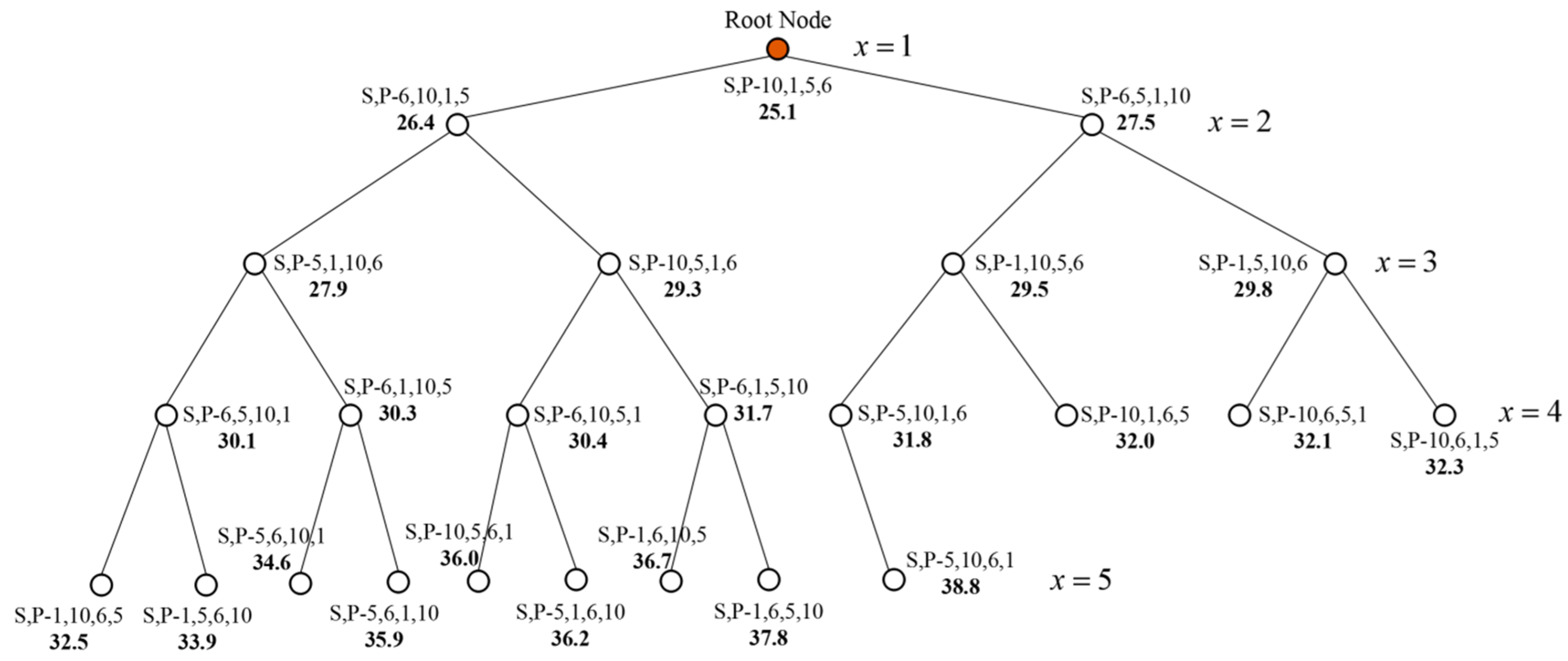
In the comparative experiment, the commonly used GaoDe map and 360 map for tourism route planning are selected as the control group, and the proposed algorithm is set as the experimental group. The control group uses relative route search methods to conduct the lowest-cost route searching performance on the same POIs $P_{a(1)}$ Jinsha Site, $P_{a(5)}$ Happy Valley, $P_{a(6)}$ Eastern Suburb Memory, and $P_{a(10)}$ Du Fu Thatched Cottage.

Table 9. The lowest cost $f_{subin·T_{ro(i, j)}}$ of sub-intervals output by the control group.

GDM	$S,P_{a(1)}$	$S,P_{a(5)}$	$S,P_{a(6)}$	$S,P_{a(10)}$	$P_{a(1)},P_{a(5)}$
	6.2	8.6	6.7	4.4	5.7
	$P_{a(1)},P_{a(6)}$	$P_{a(1)},P_{a(10)}$	$P_{a(5)},P_{a(6)}$	$P_{a(5)},P_{a(10)}$	$P_{a(6)},P_{a(10)}$
	12.1	3.9	12.3	8.7	10.9
360M	$S,P_{a(1)}$	$S,P_{a(5)}$	$S,P_{a(6)}$	$S,P_{a(10)}$	$P_{a(1)},P_{a(5)}$
	6.5	9.1	6.8	4.6	6.6
	$P_{a(1)},P_{a(6)}$	$P_{a(1)},P_{a(10)}$	$P_{a(5)},P_{a(6)}$	$P_{a(5)},P_{a(10)}$	$P_{a(6)},P_{a(10)}$
	12.7	4.0	12.8	9.4	11.3

shows the lowest cost of each sub-interval obtained by the control group methods. The control group outputs the interval cost decision trees based on the constructed interval decision tree algorithm and outputs three optimal tour routes. The sub-interval costs and interval costs are shown in

Table 10. The output optimal tour routes by the experimental group method and the control group methods.

PRA	$in·T_{ro}$	$s_u(1)$	$s_u(2)$	$s_u(3)$	$s_u(4)$	$f_{in·T_{ro}}$
	S,P-10,1,5,6	4.2	3.8	5.2	11.9	25.1
	S,P-6,10,1,5	6.6	10.8	3.8	5.2	26.4
	S,P-6,5,1,10	6.6	11.9	5.2	3.8	27.5
GDM	$in·T_{ro}$	$s_u(1)$	$s_u(2)$	$s_u(3)$	$s_u(4)$	$f_{in·T_{ro}}$
	S,P-10,1,5,6	4.4	3.9	5.7	12.3	26.3
	S,P-6,10,1,5	6.7	10.9	3.9	5.7	27.2
	S,P-6,5,1,10	6.7	12.3	5.7	3.9	28.6
360M	$in·T_{ro}$	$s_u(1)$	$s_u(2)$	$s_u(3)$	$s_u(4)$	$f_{in·T_{ro}}$
	S,P-10,1,5,6	4.6	4	6.6	12.8	28
	S,P-6,10,1,5	6.8	11.3	4	6.6	28.7
	S,P-6,5,1,10	6.8	12.8	6.6	4	30.2

.

Table 11. The sub-interval cost differences $\mathsf{\Delta }{f}_{subin·T_{ro(i, j)}}$, interval cost differences $\mathsf{\Delta }{f}_{in·T_{ro}}$ and route cost optimization rate $R_{imp}$ on the experimental group comparing to the control group.

$in·T_{ro}$		$\mathsf{\Delta }{s}_u(1)$	$\mathsf{\Delta }{s}_u(2)$	$\mathsf{\Delta }{s}_u(3)$	$\mathsf{\Delta }{s}_u(4)$	$\mathsf{\Delta }{f}_{in·T_{ro}}$	$R_{imp}$
S,P-10,1,5,6	GDM-PRA	0.2	0.1	0.5	0.4	1.2	4.56%
	360M-PRA	0.4	0.2	1.4	0.9	2.9	10.36%
$in·T_{ro}$		$\mathsf{\Delta }{s}_u(1)$	$\mathsf{\Delta }{s}_u(2)$	$\mathsf{\Delta }{s}_u(3)$	$\mathsf{\Delta }{s}_u(4)$	$\mathsf{\Delta }{f}_{in·T_{ro}}$	$R_{imp}$
S,P-6,10,1,5	GDM-PRA	0.1	0.1	0.1	0.5	0.8	2.94%
	360M-PRA	0.2	0.5	0.2	1.4	2.3	8.01%
$in·T_{ro}$		$\mathsf{\Delta }{s}_u(1)$	$\mathsf{\Delta }{s}_u(2)$	$\mathsf{\Delta }{s}_u(3)$	$\mathsf{\Delta }{s}_u(4)$	$\mathsf{\Delta }{f}_{in·T_{ro}}$	$R_{imp}$
S,P-6,5,1,10	GDM-PRA	0.1	0.4	0.5	0.1	1.1	3.85%
	360M-PRA	0.2	0.9	1.4	0.2	2.7	8.94%

takes the optimal route as an example to calculate the sub-interval cost differences $\mathsf{\Delta }{f}_{subin·T_{ro(i, j)}}$, interval cost differences $\mathsf{\Delta }{f}_{in·T_{ro}}$ and route cost optimization rate $R_{imp}$ on the experimental group compared to the control group. The symbol $s_u(x)$ in Table 10 and Table 11 represents the sub-interval.

Analyze the comparison results between the experimental group and the control group. Table 9 shows the costs $f_{subin·T_{ro(i, j)}}$ of sub-intervals searched by the control group methods, and the optimal routes and suboptimal routes of the control group are output based on the cost. Table 10 and Table 11 show the comparison of the optimal route and suboptimal route between the experimental group and the control group. The results show that the optimal route output by the experimental group and the control group is “S,P-10,1,5, 6”, and the suboptimal routes are “S,P-6,10,1,5” and “S,P-6,5,1,10”. It indicates that the experimental group and the control group have the same principle in searching for the optimal route. However, in terms of the output route cost, the control group methods produce a higher cost than that of the experimental group method, which is manifested in the sub-interval cost and the total route cost.

(1)

Comparison between GDM and the experimental group PRA: The sub-interval costs of the optimal route “S,P-10,1,5,6” are higher than those of PRA, and the route cost is 1.2 higher than that of PRA; the sub-interval costs of the suboptimal route “S,P-6,10,1,5” are all higher than those of PRA, and the route cost is 0.8 higher than that of PRA; the sub-interval costs of the suboptimal route “S,P-6,5,1,10” are all higher than those of PRA, and the route cost is 1.1 higher than that of PRA.

(2)

Comparison between 360M and the experimental group PRA: The sub-interval costs of the optimal route “S,P-10,1,5,6” are higher than those of PRA, and the route cost is 2.9 higher than that of PRA; the sub-interval costs of the suboptimal route “S,P-6,10,1,5” are all higher than those of PRA, and the route cost is 2.3 higher than that of PRA; the sub-interval costs of the suboptimal route “S,P-6,5,1,10” are all higher than those of PRA, and the route cost is 2.7 higher than that of PRA.

(3)

Comparing to the GDM, the PRA reduces the travel cost by 4.56% in terms of optimal route cost and 2.94% and 3.85% in terms of suboptimal route costs, respectively. Comparing to the 360M, the PRA reduces the travel cost by 10.36% in terms of optimal route cost, and 8.01% and 8.94% in terms of suboptimal route costs respectively. According to the comparison results, it can be concluded that the proposed tour route recommendation algorithm can effectively reduce the travel cost of the traditional routes and has obvious advantages over the traditional methods.

4.3.5. Evaluation and Analysis of Tourist Satisfaction

The data collection for the satisfaction evaluation experiment is conducted on a sample of 60 tourists, representing 60 kinds or pieces of tourists’ interests. And then the POIs are output through the proposed algorithm (PRA), the item-based collaborative filtering recommendation (IBCF), and the user-based collaborative filtering recommendation (UBCF). Then the satisfaction evaluations are conducted by sample tourists, and the average precision (${\overline{P}}_{recision}$), average recall (${\overline{R}}_{ecall}$), and average deviation of attribute matching degree (${\overline{D}}_{ev\mathrm{POI}}$) are calculated. The results are shown in

Table 12. The average precision (${\overline{P}}_{recision}$), average recall (${\overline{R}}_{ecall}$), and average deviation of attribute matching degree (${\overline{D}}_{ev\mathrm{POI}}$) of the recommended POIs.

	${\overline{\mathit{P}}}_{\mathit{r}\mathit{e}\mathit{c}\mathit{i}\mathit{s}\mathit{i}\mathit{o}\mathit{n}}$	${\overline{\mathit{R}}}_{\mathit{e}\mathit{c}\mathit{a}\mathit{l}\mathit{l}}$	${\overline{\mathit{D}}}_{\mathit{e}\mathit{v}\mathbf{POI}}$
PRA	0.5357	0.1429	1.0116
IBCF	0.3929	0.1048	1.8235
UBCF	0.3214	0.0857	2.0720

. Based on the recommended POIs, the proposed algorithm (PRA), GaoDe Map Method (GDM), and 360 Map Method (360M) are used to recommend routes, and the satisfaction evaluations are conducted by sample tourists. Then the average precision (${\overline{P}}_{recision}$), average recall (${\overline{R}}_{ecall}$), and average cost deviation of the recommended routes (${\overline{D}}_{ev\mathrm{Route}}$) are calculated. The results are shown in

Table 13. The average precision (${\overline{P}}_{recision}$), average recall (${\overline{R}}_{ecall}$), and average cost deviation of the recommended routes (${\overline{D}}_{ev\mathrm{Route}}$) of the recommended routes.

	${\overline{\mathit{P}}}_{\mathit{r}\mathit{e}\mathit{c}\mathit{i}\mathit{s}\mathit{i}\mathit{o}\mathit{n}}$	${\overline{\mathit{R}}}_{\mathit{e}\mathit{c}\mathit{a}\mathit{l}\mathit{l}}$	${\overline{\mathit{D}}}_{\mathit{e}\mathit{v}\mathbf{Route}}$
PRA	0.7500	0.1250	6.2714
GDM	0.5000	0.0833	9.0000
360M	0.3214	0.0536	10.7643

.

Sample tourists evaluate the satisfaction of each algorithm’s recommended POIs and routes and make choices based on the recommendation results. By using the satisfaction evaluation model we have proposed, the results in Table 12 and Table 13 that reflect tourists’ satisfactions are obtained. Analyzing the data in Table 12, in terms of POI recommendation satisfaction evaluations, PRA has the highest average precision of 0.5357, which is higher than that of the control group’s recommendation method IBCF of 0.3929 and UBCF of 0.3214. It indicates that the overall sample of tourists has the highest satisfaction with the POIs recommended by our proposed algorithm, and it also indicates that the precision of the POIs recommended by the proposed algorithm is the highest. The average recall rate of PRA is the highest, at 0.1429, which is higher than that of IBCF in the control group, which is 0.1048, and UBCF, which is 0.0857. It indicates that the overall sample of tourists has the highest satisfaction with the POIs recommended by our proposed algorithm, and the algorithm has the highest precision in recommending satisfied POIs from all destination POIs. The average deviation of attribute matching degree for PRA is the lowest, at 1.0116, which is lower than that of the control group’s recommendation method, IBCF, which is 1.8235, and UBCF, which is 2.0720. It indicates that the proposed algorithm has the strongest ability to recommend POIs that meet tourists’ interests.

Analyzing the data in Table 13, in terms of satisfaction evaluation of tourist routes, PRA has the highest average precision of 0.7500, which is higher than that of the control group’s route method GDM of 0.5000 and 360M of 0.3214. It indicates that the overall sample of tourists has the highest satisfaction with the recommended routes by the proposed algorithm, and it also indicates that the precision of the recommended routes by the proposed algorithm is the highest. The average recall of PRA is the highest, at 0.1250, which is higher than that of GDM in the control group, which is 0.0833, and that of 360M, which is 0.0536. It indicates that the overall sample of tourists has the highest satisfaction with the recommended routes of the proposed algorithm, and the algorithm has the highest precision in recommending satisfied routes from all the searched routes. The average cost deviation of the PRA route is the lowest, at 6.2714, and it is lower than that of the GDM, which is 9.0000, and that of 360M, which is 10.7643, indicating that the proposed algorithm has the strongest ability to recommend routes that meet tourists’ interests while saving travel costs.

From the perspective of satisfaction evaluation, the comparison experiment proves that the proposed algorithm can better satisfy tourists than traditional recommendation algorithms and map route planning methods. It performs better in terms of each satisfaction index and ability than traditional methods. The recommended POIs are better than traditional recommendation algorithms IBCF and UBCF in terms of satisfaction degree, and the recommended routes are better than traditional map route planning methods GDM and 360M in terms of satisfaction degree.

5. Conclusions

On the basis of analyzing the current research background and existing problems of POI tour routes, this paper proposes and constructs a POI tour route recommendation model based on the improved symmetry-based Naive Bayes mining and spatial decision forest search. The POI natural attribute classification model is constructed based on text mining, and the destination POIs are classified into natural attribute classifications. Furthermore, an improved symmetry-based Naive Bayes classification algorithm for the destination POI tourism attribute classification is constructed through once-visited POIs, and the destination POIs are classified into different tourism attribute classifications. By constructing a spatial decision forest algorithm, the POIs with natural attributes under different tourism attribute classifications are sorted, and a recommendation model is established to output the optimal POIs. Based on the recommended POIs, a POI tour route recommendation model based on the spatial decision tree algorithm is established, which outputs the tour route with the lowest sub-interval costs and interval cost. Finally, the validation experiment and the comparative experiment are performed to output the optimal POIs and tour routes by using the proposed algorithm. Then the proposed algorithm is compared with the commonly used route planning methods, GDM and 360M, demonstrating the advantages of the proposed algorithm compared to the traditional route planning methods. The output POI tour routes can effectively reduce travel costs using the proposed algorithm.

References

1. Darapisut, S.; Amphawan, K.; Leelathakul, N.; Rimcharoen, S. A Hybrid POI Recommendation System Combining Link Analysis and Collaborative Filtering Based on Various Visiting Behaviors. ISPRS Int. J. Geo-Inf. 2023, 12, 431. [Google Scholar] [CrossRef]
2. Lee, J.; Kim, J. Developing a Convenience Store Product Recommendation System through Store-Based Collaborative Filtering. Appl. Sci. 2023, 13, 11231. [Google Scholar] [CrossRef]
3. Aldayel, M.; Al-Nafjan, A.; Al-Nuwaiser, W.; Alrehaili, G.; Alyahya, G. Collaborative Filtering-Based Recommendation Systems for Touristic Businesses, Attractions, and Destinations. Electronics 2023, 12, 4047. [Google Scholar] [CrossRef]
4. Alabduljabbar, R. Matrix Factorization Collaborative-Based Recommender System for Riyadh Restaurants: Leveraging Machine Learning to Enhance Consumer Choice. Appl. Sci. 2023, 13, 9574. [Google Scholar] [CrossRef]
5. Lin, S. Implementation of Personalized Scenic Spot Recommendation Algorithm Based on Generalized Regression Neural Network for 5G Smart Tourism System. Comput. Intel. Neurosc. 2022, 2022, 3704494. [Google Scholar] [CrossRef] [PubMed]
6. Bin, C.; Gu, T.; Jia, Z.; Zhu, G.; Xiao, C. A Neural Multi-context Modeling Framework for Personalized Attraction Recommendation. Multimed. Tools. Appl. 2020, 79, 14951. [Google Scholar] [CrossRef]
7. Li, G.; Hua, J.; Yuan, T.; Wu, J.; Jiang, Z.; Zhang, H.; Li, T. Novel Recommendation System for Tourist Spots Based on Hierarchical Sampling Statistics and SVD++. Math. Probl. Eng. 2019, 2019, 2072375. [Google Scholar] [CrossRef]
8. Mizutani, Y.; Yamamoto, K. A Sightseeing Spot Recommendation System That Takes into Account the Change in Circumstances of Users. ISPRS Int. J. Geo-Inf. 2017, 6, 303. [Google Scholar] [CrossRef]
9. Huang, C.; Liu, M.; Gong, H.; Xu, F. Season-aware Attraction Recommendation Method with Dual-trust Enhancement. J. Intell. Fuzzy Syst. 2017, 33, 2437–2449. [Google Scholar] [CrossRef]
10. Kesorn, K.; Juraphanthong, W.; Salaiwarakul, A. Personalized Attraction Recommendation System for Tourists Through Check-In Data. IEEE Access 2017, 5, 26703–26721. [Google Scholar] [CrossRef]
11. Remigijus, P.; Linas, S.; Simona, S.; Dmitrij, K.; Ernestas, F. A Novel Greedy Genetic Algorithm-based Personalized Travel Recommendation System. Expert. Syst. Appl. 2023, 230, 120580. [Google Scholar]
12. Zhang, Y.; Liu, S. A Picture-Based Approach to Tourism Recommendation System. Front. Soc. Sci. Technol. 2023, 5, 124–130. [Google Scholar]
13. Liang, S.; Jin, J.; Ren, J.; Du, W.; Qu, S. An Improved Dual-Channel Deep Q-Network Model for Tourism Recommendation. Big Data 2023, 11, 268–281. [Google Scholar] [CrossRef] [PubMed]
14. Han, S.; Liu, C.; Chen, K.; Gui, D.; Du, Q. A Tourist Attraction Recommendation Model Fusing Spatial, Temporal, and Visual Embeddings for Flickr-Geotagged Photos. ISPRS Int. J. Geo-Inf. 2021, 10, 20. [Google Scholar] [CrossRef]
15. Mulia, W.; Chelsia, P.; Widi, B.; Rizqina, M. Discovering the Importance of Halal Tourism for Indonesian Muslim Travelers: Perceptions and Behaviors When Traveling to a Non-Muslim Destination. J. Islamic Mark. 2023, 14, 61–81. [Google Scholar]
16. Wang, Y.; Huang, Y.; Yang, K.; Chen, Z.; Luo, C. Generator Fault Classification Method Based on Multi-Source Information Fusion Naive Bayes Classification Algorithm. Energies 2022, 15, 9635. [Google Scholar] [CrossRef]
17. Wang, Q.; Wang, F.; Li, Z.; Jiang, P.; Ren, F.; Nie, F. Efficient Random Subspace Decision Forests with a Simple Probability Dimensionality Setting Scheme. Inform. Sci. 2023, 638, 118993. [Google Scholar] [CrossRef]
18. Li, L.; Gao, Q. Researching Tourism Space in China’s Great Bay Area: Spatial Pattern, Driving Forces and Its Coupling with Economy and Population. Land 2023, 12, 1878. [Google Scholar] [CrossRef]
19. Wang, H.; Chen, X.; Ge, J.; Yan, Z.; He, X.; Song, Y.; Zhou, Q. Research on the Spatiotemporal Distribution and Cultural Tourism Strategy of Modern Educational Architectural Heritage in Nanjing. Sustainability 2023, 15, 14392. [Google Scholar] [CrossRef]
20. Rabbiosi, C.; Meneghello, S. Questioning Walking Tourism from a Phenomenological Perspective: Epistemological and Methodological Innovations. Humanities 2023, 12, 65. [Google Scholar] [CrossRef]
Figure 1. The overall framework and flowchart of the research content.
Symmetry 15 02168 g001
Figure 2. The constructed POI natural attribute classification structure tree Tree   G N ( i ) .
Symmetry 15 02168 g002
Figure 3. The constructed tourism attribute interest network N e t · λ T ( i ) .
Symmetry 15 02168 g003
Figure 4. The modeling process to generate the decision tree Tree C ( i ) and decision forest F o r e s t C ( i ) . (A) shows the initial state of the root node C ( 1 ) and the growth child node G N ( t ) . (B) shows a complete binary tree. (C) shows a recommendation structure tree Tree C ( 1 ) consisting of k number of derived binary trees from k number of G N ( t ) . (D) shows a recommendation decision forest F o r e s t C ( i ) by w number of recommendation decision trees Tree C ( i ) .
Symmetry 15 02168 g004
Figure 8. The trend of POI label weights t f i d f ( λ N ( i ) ) under each natural attribute classification. (A) shows a histogram of the weight distribution of each POI for each classification G N ( i ) , and (B) shows the weight trend of each POI in each classification G N ( i ) .
Symmetry 15 02168 g008
Figure 9. The recommendation degree distribution of each target POI belonging to C ( i ) . In (A), the red curve represents the classification C ( 1 ) . In (B), the blue curve represents the classification C ( 2 ) . In (C), the green curve represents the classification C ( 3 ) . (D) shows the comparison of the three types of curves.
Symmetry 15 02168 g009
Figure 10. The constructed destination POI recommendation degree decision tree Tree C ( i ) and decision forest F o r e s t   C ( i ) .
Symmetry 15 02168 g010
Figure 11. The final output tour route interval cost decision tree t r · T r o .
Symmetry 15 02168 g011