Abstract
The Weibull distribution is a continuous probability distribution that finds wide application in various fields for analyzing real-world data. Specifically, wind speed data often adhere to the Weibull distribution. In our study, our aim is to compare the mean wind speed datasets from different areas in Thailand. To achieve this, we proposed simultaneous confidence intervals for all pairwise differences between the means of Weibull distributions. The generalized confidence interval (GCI), method of variance estimates recovery (MOVER), and a Bayesian approach, utilizing both gamma and uniform prior distributions, are proposed to construct simultaneous confidence intervals. Through simulations, we find that the Bayesian highest posterior density (HPD) interval using a gamma prior distribution demonstrates satisfactory performance, while the GCI proves to be a viable alternative. Finally, we applied these proposed approaches to real wind speed data in northeastern and southern Thailand to illustrate their effectiveness and practicality.
Keywords:
Bayesian; generalized confidence interval; method of variance estimates recovery; Weibull distribution MSC:
62F25; 62F15
1. Introduction
The Weibull distribution is widely used in various fields due to its heavy-tailed nature and remains asymmetric regardless of the chosen parameter values. Consequently, transforming it into a perfectly symmetric distribution is a complex task. However, it is feasible to make the Weibull distribution more symmetrical or to approximate symmetry. Techniques explored include a close-to-normal power approximation, logarithmic transformation, and the Box–Cox transformation. The Weibull distribution finds applications in diverse fields, such as insurance (Kreer et al. [1], Hamza and Sabri [2]), food science (Mafart et al. [3], Uribete et al. [4]), ecology (Mikolaj [5]), and medical science (Carroll [6]). In addition, numerous studies have presented examples of wind speed data that follow a Weibull distribution. For instance, Waewsak et al. [7] analyzed the statistical wind data obtained from the Thasala district in Nakhon Si Thammarat province, southern Thailand. Chauhan and Saini [8] examined the wind speed data from the Harshnath site in the Sikar district of Rajasthan, India. Kidmo et al. [9] studied the wind speed distribution based on six Weibull methods for wind power evaluation in Garoua, Cameroon. Bidaoui et al. [10] assessed and discussed the wind energy potential in five major cities in northern Morocco. Shu and Jesson [11] estimated Weibull parameters, which are used to evaluate wind power density in the UK. In the field of inferential statistics, researchers have shown interest in constructing confidence intervals for the mean and its functions in Weibull distributions. For example, Colosimo and Ho [12] conducted a study where they utilized censored reliability datasets to determine the confidence interval of the mean lifetime in Weibull distributions. In a different study, Muralidharan and Lathika [13] estimated the confidence interval for mean rainfall data by employing a modified version of the Weibull distribution. Krishnamoorthy et al. [14] conducted research in which they utilized the generalized variable method to establish confidence intervals for the mean of the Weibull distribution, and subsequently contrasted these results with Wald confidence intervals. In their study, La-ongkaew et al. [15] utilized the generalized confidence interval (GCI) and the method of variance estimates recovery (MOVER), along with the Wald confidence interval, to derive confidence intervals for the difference between means and the ratio of means of Weibull distributions.
The multiple comparisons of several parameters of interest correspond to the concept of simultaneous confidence intervals (SCIs). SCIs are intervals that comprise individual intervals for the separate components of the parameter. They allow for the estimation of all treatments at the same time. This problem has been extensively discussed in the literature. Hannig et al. [16] introduced the fiducial generalized pivotal quantities (FGPQ) method, which allows for the construction of SCIs for all pairwise ratios of means of lognormal distributions. Sadooghi-Alvandi and Malekzadeh [17] developed a new parametric bootstrap method for constructing SCIs for the ratios of means of multiple lognormal distributions. Their results indicated that the parametric bootstrap procedure consistently outperforms other procedures, which are based on the concepts of GPQ and FGPQ. In the same year, Zhang and Falk [18] introduced FGPQ-based SCIs for the ratios of means of multiple lognormal distributions, considering heteroscedastic variances and unequal group sizes. Li et al. [19] suggested a parametric bootstrap technique to construct SCIs for the differences of means from several two-parameter exponential distributions. Their outcomes showed that the suggested SCIs are typically closer to the nominal level. Also, in 2015, Abdel-Karim [20] presented a two-step MOVER, called FGCIs-MOVER and MOVER-MOVER, to estimate SCIs for ratios of means of lognormal distributions. Moving to 2018, Thangjai et al. [21] introduced a procedure to estimate SCIs for the differences in means of multiple normal populations with unknown coefficients of variation. They employed the GCI approach and the MOVER approach. Lastly, Maneerat et al. [22] proposed SCIs for pairwise comparisons of the means of delta-lognormal distributions. They used the parametric bootstrap approach, FGCI approach, MOVER approach, and Bayesian credible intervals with mixed and uniform priors. Their simulation results showed that Bayesian credible intervals-uniform prior and parametric bootstrap work well in different situations, even with large differences in variance.
As far as we know, there has not been any research examining the development of SCIs for all differences between the means of the Weibull distributions. In this particular study, we propose the GCI, MOVER, and Bayesian methods for establishing SCIs for all differences between the means of the Weibull distributions. The remaining sections of this paper are structured as follows. Section 2 outlines the materials and methods that are used to construct SCIs for all the differences between the means of the Weibull distributions. The simulation results were conducted on sample cases with sizes of 3 and 5 and are presented in Section 3. These methods were applied to wind speed datasets collected from three provinces in northeastern and southern Thailand, which are shown in Section 4. Lastly, we present the discussion and conclusion of this study.
2. Materials and Methods
Suppose that = , ,…, is the random vector from the p-dimensional Weibull distribution with and , denoted as . Waloddi Weibull proposed the Weibull distribution and defined the probability density function (pdf) of as
for and . The respective mean and variance can be derived as
and
The methods described in this section aim to construct SCIs. Our focus lies in constructing the SCIs for all pairwise differences between the means, then
where .
2.1. GCI
To construct the SCIs based on the GCI method, the GPQ concept is employed in the following manner.
Definition 1.
Let = , ,…, be a random variablesvector from p-independent Weibull distributions, which are based on a parameter of interest , and a nuisance parameter . Let = (, ,…, ) be an observed value of . Then, is called the GPQ when it fulfills the two conditions introduced by Weerahandi [23].
The GPQs for the scale and shape parameters of the Weibull distributions, which fulfill two conditions, were presented by Krishnamoorthy et al. [24]. Let be the GPQ for the shape parameter () and be the GPQ for the scale parameter (), respectively. They can be obtained from the following equations.
and
Let be the maximum likelihood estimators of from , and be the observed values of . Similarly, let be the maximum likelihood estimators of from , and be the observed values of . The research conducted by Thoman et al. [25] demonstrated that the distributions of and are independent of any parameters. Let and be the maximum likelihood estimators from . Consequently, it becomes clear that is distributed as and is distributed as .
Herein, we developed the GCI method to establish SCIs for . Firstly, the GPQ for estimating is determined as
From Equation (4), we can obtain
Therefore, the 100 SCI based on GCI for is given by
where is the 100/2-th quantiles of . Algorithm 1 is utilized to construct and .
| Algorithm 1: GCI approach |
2.2. MOVER
The MOVER method was introduced by Donner and Zou [26]. This technique allows for the construction of a confidence interval for a function for two parameters. Herein, we applied this method to construct a confidence interval for the difference between two parameters of interest. Therefore, the MOVER method is considered. For the difference in means, the confidence interval for parameter is given by
and
Consider the p parameters of interest, for and , the lower bound and the upper bound become
and
where and are defined as Equation (2). Let , , , and be the confidence interval for and of the Weibull distributions. In our work, the Wald method was considered to construct them. According to the Wald confidence interval, the 100 two-sided confidence interval for of the Weibull distribution is given by , where . The derivation is provided below.
and
where is the -th quantile of a standard normal distribution. The estimate of variance for is defined by
Using the Fisher information matrix enables the determination of estimates for the variance and covariance of and , which is
2.3. Bayesian Inference
In Bayesian statistics, prior distributions play a pivotal role by enabling the integration of pre-existing knowledge or assumptions about the parameters of interest before observing the data. Combining this prior distribution with the likelihood function derived from observed data yields the posterior distribution in Bayesian inference. The posterior distribution effectively encapsulates refined beliefs about the parameters after considering the data. Here, we explore the Bayesian inference of the parameters of the Weibull distribution, utilizing both a gamma prior distribution and a uniform prior distribution.
2.3.1. Bayesian Gamma Prior
The gamma distribution is a versatile family that can manifest in various shapes, including the generalized gamma, exponential, and Rayleigh distributions. Notably, it serves as a conjugate prior to the exponential likelihood function, ensuring that its structure remains intact in the posterior. This conjugate property simplifies the computations required for Bayesian updating. Additionally, when employing a gamma distribution as a prior for the parameters, it harmonizes well with the characteristics of the Weibull distribution, making it a natural choice for Bayesian inference in these contexts. In this particular part, we consider a gamma prior for the scale and shape parameters, assuming their independent distributions. Then, the gamma priors for a and k are
and
where corresponds to , and the hyperparameters are assumed to be known real numbers. Let be an associated likelihood function, then the joint density function of the data, and k, is
Therefore, the posterior density function, given the data, is
The Bayes estimates cannot be obtained in a simple, closed form due to the challenge of evaluating the integrals in Equation (21) analytically. As a result, an alternative method for parameter estimation is needed, and the Markov chain Monte Carlo (MCMC) method is often employed. The MCMC method has been proven to be successful in Bayesian computing, particularly through its ability to sample from full conditional distributions. One commonly used variant of MCMC is the Gibbs sampler. In this study, we propose using the Gibbs sampling procedure to generate MCMC samples and compute the Bayes estimate, as described by (Geman and Geman [27]). The wholly conditional posterior distributions of and k are
and
Equation (22) corresponds to a gamma density with parameters and . Generating samples of can be easily accomplished using any gamma-generating routine. However, for Equation (23), relying solely on the Gibbs sampling procedure to update them is not sufficient. Instead, we need to employ the Metropolis–Hastings algorithm to update the shape parameter. This algorithm is particularly useful when direct sampling from a distribution is challenging, making it the chosen method for generating samples of the shape parameter. In this research, we applied both the Gibbs sampling procedure and the Metropolis–Hastings algorithm to generate samples from full conditional distributions using the R (version 4.1.2) programming software package. OpenBUGS (Bayesian inference Using Gibbs Sampling) is a software package designed for performing Bayesian analysis with MCMC methods. It offers a flexible and intuitive approach for specifying and fitting Bayesian statistical models, particularly suitable for complex models. To utilize OpenBUGS in R, it is necessary to have the “R2OpenBUGS” package installed, provinding an interface between R and OpenBUGS.
Let us once again consider the p parameters of interest, for ; the differences between means were computed as Equation (4). Therefore, the 100 SCI based on Bayesian equal-tailed using gamma prior distribution for is given by
where and are the lower and upper bounds of the 100 equal-tailed confidence intervals of . In Bayesian statistics, alongside equal-tailed confidence intervals, there exists another type known as the highest posterior density (HPD) interval. This interval delineates the most densely populated region in the posterior distribution, encapsulating the parameter’s most probable values. The Bayesian-HPD interval is the shortest among all of the available Bayesian credible intervals for some given . The assumption is that the probability density within it is higher compared to the values outside of it [28]. As a result, it tends to be the narrowest possible interval. Using the R statistical program with a package of HDInterval, the 100 SCI based on the Bayesian-HPD interval using gamma prior distribution for is
Algorithm 3 is utilized to construct [,] and [,].
| Algorithm 3: Bayesian equal-tailed and Bayesian-HPD interval using gamma prior |
2.3.2. Bayesian Uniform Prior
In the previous subsection, we explored how Bayesian estimation incorporates prior knowledge about the parameter. However, in situations where prior knowledge is lacking, we can employ a non-informative prior in Bayesian analysis. In the context of this subsection, we assume a uniform prior distribution for the scale and shape parameters: and .
To estimate the parameters based on Bayesian with a uniform prior, the OpenBUGS (version 3.2-3.2.1) software in R programming is discussed again. By utilizing Equation (4) and considering the prior information, we make estimations to determine the differences in means for the p parameters of interest.
As a result, the 100 SCI based on Bayesian equal-tailed using uniform prior distribution for is given by
Similarly, the 100 SCI based on the Bayesian-HPD interval using uniform prior distribution for is
Algorithm 4 is utilized to construct [,] and [,].
| Algorithm 4: Bayesian equal-tailed and Bayesian-HPD interval using uniform prior |
|
3. Results
A simulation analysis was conducted to evaluate the efficacy of the suggested approaches. The evaluation of these methods involved analyzing the coverage probabilities (CPs), expected lengths (ELs), and standard error (s.e) of the confidence intervals. The simulation study consisted of 5000 simulation runs, and for the GCI, there were 2500 replications. Furthermore, we utilized Gibbs sampling in conjunction with the Metropolis–Hastings algorithm, conducting 20,000 iterations with a burn-in of 1000. The hyperparameter values were fixed at . To be considered satisfactory, the SCI should exhibit CPs that are near or above the nominal confidence level of 0.95 while also demonstrating the shortest EL. The simulation studies were conducted with parameter combinations chosen accordingly.
- Sample cases: p = 3, 5;
- Shape parameter: = 2;
- Sample size: ;
- Population mean: .
According to Table 1 and Table 2, these factors were both fixed and varied in various situations. Obtaining CPs for the SCIs is facilitated by following Algorithm 5.
| Algorithm 5: The CP of the SCIs estimates for the differences between means of Weibull distributions |
|

Table 1.
The CPs and ELs of 95% SCIs for all differences between means of Weibull distributions for .
Table 2.
The CPs and ELs of 95% SCIs for all differences between means of Weibull distributions for .
The CPs and ELs of the proposed methods in Table 1 and Table 2 are summarized in Figure 1 and Figure 2. For , the , , and demonstrate satisfactory CPs. Nevertheless, when comparing the ELs and the standard errors, it becomes apparent that consistently yields smaller values compared to the other methods in all scenarios. One noteworthy result from the study is that the performs well in situations where the means and sample sizes of each group are unequal. For and , the CPs are close to 1 when , regardless of the sample sizes. However, when , outperforms the other methods. Lastly, the method consistently underestimates the CPs, yielding values below the target across all scenarios. The findings for are similar to those for . Considering the equal sample sizes, showed the best performance in terms of CPs, ELs, and standard errors. The has good performance when the means of each population are not equal . The had CPs higher than the goal when for , and 30. When the sample sizes are not equal, both and are similarly effective in achieving CPs greater than or close to 0.95. Nevertheless, yielded narrower ELs and standard errors compared to the . Thus, we recommend using the Bayesian-HPD interval with a gamma prior distribution for constructing SCIs for the difference between the means of the Weibull distributions, both in cases of equal and unequal sample sizes. This recommendation is based on the observation that the results for yielded similar outcomes to those for .
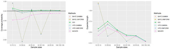
Figure 1.
Comparison of method performance in terms of CPs and ELs according to the number of samples ().
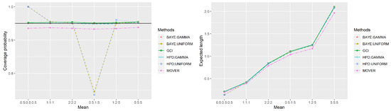
Figure 2.
Comparison of method performance in terms of CPs and ELs according to the mean ().
4. Applications
Thailand, located in tropical Southeast Asia, can be categorized into five distinct regions: the North, Northeast, Central, East, and South. Each region has distinct geographical features. The North is characterized by valleys, while the Central region consists of lowlands. The Northeast region is renowned for its mountains, whereas the East has a combination of mountains and plains. The South, on the other hand, is a peninsula. A study conducted by the Department of Alternative Energy Development and Efficiency, Ministry of Energy, explored the potential sources of wind energy and found that most areas in Thailand have low wind speed potentials. However, specific regions stand out as promising sources of wind energy. The southern region of Nakhon Si Thammarat province, along with areas near the shores of Songkhla Lake, have been identified as good sources of wind energy. According to a report by the Electricity Generating Authority of Thailand, approximately 86% of the areas with significant wind energy potential are concentrated in the Northeastern region. Moreover, private sector studies have also identified the Lopburi, Nakhon Ratchasima, and Chaiyaphum provinces as having significant wind energy potential. Multiple reports from various agencies corroborate the notion that there are numerous areas in Thailand that could serve as excellent sources of wind energy.
4.1. Example 1
In this section, we utilized monthly wind speed (in knot) data from three provinces in northeastern Thailand—namely Surin, Nong Khai, and Sakon Nakhon—as examples for to examine the efficiency of the proposed method. The data, collected over four years from 2018 to 2021, were obtained from the Meteorological Department of Thailand [29]. To determine the fit of the distributions to the collected data, we employed the Akaike information criterion (AIC). The AIC results are presented in Table 3, demonstrating that the datasets from all three areas were well-suited to Weibull distributions. Additionally, we generated Q-Q plots to visualize the datasets, depicted in Figure 3. For further insight, we also compiled summary statistics for the three datasets, which can be found in Table 4. Subsequently, Table 5 provides an overview of the 95% SCIs for all pairwise differences between the means in wind speed data among the three provinces in northeastern Thailand, computed using all the methods.
Table 3.
AIC values for the wind speed datasets representing three provinces in northeastern.
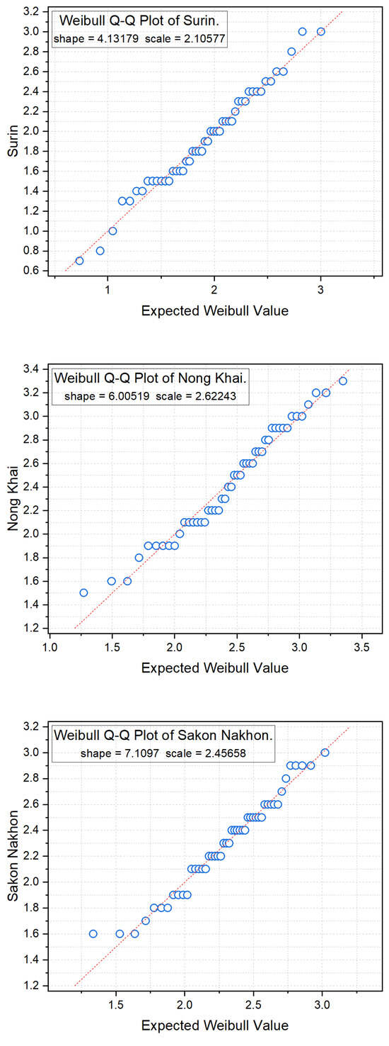
Figure 3.
Weibull Q-Q plots of the dataset from three provinces in northeastern Thailand.
Table 4.
Summary statistics for the wind speed datasets from three provinces in northeastern Thailand.
Table 5.
The 95% simultaneous confidence intervals for all pairwise differences between means of the wind speed data from three provinces in northeastern Thailand.
When considering the length of the pairwise differences of means from Table 5, the MOVER method had the smallest length. However, in the simulation results of the MOVER method, the CP did not reach 0.95 in all cases. As a result, the MOVER method will not be considered. Therefore, when considering both CP and the smallest length, it is recommended to use the Bayesian HPD-interval using gamma prior to estimating the SCIs for all pairwise differences between the means of wind speed data from the three provinces in northeastern Thailand. It has been confirmed that the Bayesian HPD-interval using a gamma prior is suitable for constructing SCIs for all pairwise differences between the means of Weibull distributions, particularly in cases of equal sample sizes.
4.2. Example 2
For , we used monthly wind speed (in knot) data from three provinces in southern Thailand—namely Pattni, Chumphon, and Songkhla—as an example. The data for each province were collected from 2008 to 2012 and were obtained from the Meteorological Department of [29]. Wind speed data from Pattani Province were collected from one station, Chumphon Province from two stations, and Songkhla Province from three stations. This results in an unequal number of samples in each province. To evaluate the appropriateness of the distributions, we revisited the AIC results. The findings indicated that the Weibull distributions were well-matched to the datasets from all three areas, as detailed in Table 6. Q-Q plots illustrating the datasets were generated and can be seen in Figure 4. The summary statistics for the wind speed dataset of three provinces in southern Thailand are presented in Table 7. The 95% SCIs for all pairwise differences between the means in wind speed data among the three provinces in southern Thailand reported in Table 8 indicated that the length of the Bayesian HPD-interval using gamma prior was the shortest. Once again, it has been confirmed that the Bayesian HPD-interval, utilizing a gamma prior, is well-suited for establishing SCIs for all pairwise differences in the means of Weibull distributions, even when dealing with uneven sample sizes.
Table 6.
AIC values for the wind speed datasets representing three provinces in southern Thailand.
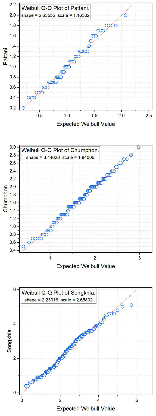
Figure 4.
Weibull Q-Q plots of the dataset from three provinces in southern Thailand.
Table 7.
Summary statistics for the wind speed datasets from three provinces in southern Thailand.
Table 8.
The 95% simultaneous confidence intervals for all pairwise differences between means of the wind speed data from three provinces in southern Thailand.
5. Discussion
La-ongkaew et al. [30] presented Bayesian methods relying on a gamma prior distribution to establish the difference in parameter values of Weibull distributions. The results of their investigation demonstrated that both the Bayesian HPD-interval and GCI methods outperformed others in different scenarios. Buliding on this concept, we extended our work to construct estimates for the confidence interval for the differences of means of Weibull populations simultaneously.
The concepts of GCI, MOVER, and Bayesian methods were used to estimate the SCIs for all pairwise differences between the means of Weibull distributions. This study presented a Bayesian approach utilizing gamma and uniform prior distributions. The Bayesian HPD-interval using the gamma prior performed well in most cases, with CPs frequently meeting or closely approaching the set target while also yielding the shortest ELs. However, there are limitations for the Bayesian HPD-interval using the gamma prior in the case of small sample sizes. It is possible that these limitations stem from the hyperparameter configuration in the gamma prior distribution. Additionally, there are other algorithms available to address the issue of a non-closed-form posterior distribution, such as the independent Metropolis–Hastings algorithm, slice sampling, or Lindley’s approximation. These alternatatives provide an interesting avenue for future research. Furthermore, an increase in sample size consistently led to a decrease in ELs, with the s.e. producing consistent outcomes.
Finally, the results were further supported by the computation of an example involving wind speed data from three provinces in northeastern and southern Thailand. Armed the with knowledge of the difference in the means of wind speed between two areas, related agencies can more effectively comprehend, utilize, plan for, and even anticipate suitable wind speed levels.
6. Conclusions
Herein, six methods for constructing SCIs for all pairwise differences between the means of Weibull distributions using GCI, MOVER, Bayesian equal-tailed, and HPD-interval, based on gamma and uniform priors, are presented. Our findings indicated that the HPD-interval using gamma prior had a reasonable CP, along with a satisfactory EL. Therefore, we recommend this method for constructing the SCIs for all pairwise differences between the means of Weibull distributions. Additionally, the GCI showed a CP higher than the goal in many cases, making it a viable alternative method.
Author Contributions
Conceptualization, S.-A.N.; Methodology, M.L.-o., S.-A.N., and S.N.; Software, M.L.-o.; Formal analysis, M.L.-o. and S.N.; Investigation, S.-A.N. and S.N.; Project administration, S.-A.N.; Resources, S.-A.N.; Data curation, M.L.-o.; Writing—original draft, M.L.-o.; Writing—review and editing, S.-A.N. and S.N.; Supervision, S.-A.N. and S.N. All authors have read and agreed to the published version of the manuscript.
Funding
This research was funded by King Mongkut’s University of Technology North Bangkok, Contract no. KMUTNB-67-KNOW-09.
Institutional Review Board Statement
Not applicable.
Informed Consent Statement
Not applicable.
Data Availability Statement
Data may be made available by contacting the corresponding author.
Acknowledgments
The authors would like to express their gratitude to King Mongkut’s University of Technology North Bangkok for funding their research and providing a venue for programming.
Conflicts of Interest
The authors declare no conflict of interest.
Abbreviations
The following abbreviations are used in this manuscript:
| AIC | Akaike information criterion |
| BAYE.g | Bayesian equal-tailed using gamma prior distribution |
| BAYE.u | Bayesian equal-tailed using uniform prior distribution |
| CP | Coverage probability |
| EL | Expected length |
| GCI | Generalized confidence interval |
| GPQ | Generalized pivotal quantities |
| HPD | Highest posterior density |
| HPD.g | Highest posterior density using gamma prior distribution |
| HPD.u | Highest posterior density using uniform prior distribution |
| MCMC | Markov chain Monte Carlo |
| MOVER | Method of variance estimates recovery |
| SCI | Simultaneous confidence interval |
| s.e. | Standard error |
References
- Kreer, M.; Kızılersü, A.; Thomas, A.W.; Egídio dos Reis, A.D. Goodness-of-fit tests and applications for left-truncated Weibull distributions to non-life insurance. Eur. Actuar. J. 2015, 5, 139–163. [Google Scholar] [CrossRef]
- Hamza, A.; Sabri, S.R.M. Weibull Distribution for claims modelling: A Bayesian Approach. In Proceedings of the International Conference on Decision Aid Sciences and Applications, Chiangrai, Thailand, 23–25 March 2022. [Google Scholar]
- Mafart, P.; Couvert, O.; Gaillard, S.; Leguérinel, I. On calculating sterility in thermal preservation methods: Application of the Weibull frequency distribution model. Int. J. Food Microbiol. 2002, 72, 107–113. [Google Scholar] [CrossRef] [PubMed]
- Uribe, E.; Vega-Gálvez, A.; Di Scala, K.; Oyanadel, R.; Saavedra Torrico, J.; Miranda, M. Characteristics of convective drying of pepino fruit (Solanum muricatum Ait.): Application of Weibull distribution. Food Bioprocess Technol. 2011, 4, 1349–1356. [Google Scholar] [CrossRef]
- Mikolaj, P.G. Environmental applications of the Weibull distribution function: Oil pollution. Science 1972, 176, 1019–1021. [Google Scholar] [CrossRef] [PubMed]
- Carroll, K.J. On the use and utility of the Weibull model in the analysis of survival data. Control Clin. Trials 2003, 24, 682–701. [Google Scholar] [CrossRef] [PubMed]
- Waewsak, J.; Chancham, C.; Landry, M.; Gagnon, Y. An analysis of wind speed distribution at Thasala. Thailand. J. Sustain. Energy Environ. 2011, 2, 51–55. [Google Scholar]
- Chauhan, A.; Saini, R.P. Statistical analysis of wind speed data using Weibull distribution parameters. In Proceedings of the International Conference on Non-Conventional Energy, Kalyani, India, 16–17 January 2014. [Google Scholar]
- Kidmo, D.K.; Danwe, R.; Doka, S.Y.; Djongyang, N. Statistical analysis of wind speed distribution based on six Weibull Methods for wind power evaluation in Garoua, Cameroon. Rev. Des. Energies Renouvelables 2015, 18, 105–125. [Google Scholar]
- Bidaoui, H.; El Abbassi, I.; El Bouardi, A.; Darcherif, A. Wind speed data analysis using Weibull and Rayleigh distribution functions, case study: Five cities northern Morocco. Procedia Manuf. 2019, 32, 786–793. [Google Scholar] [CrossRef]
- Shu, Z.R.; Jesson, M. Estimation of Weibull parameters for wind energy analysis across the UK. J. Renew. Sustain. Energy 2021, 13, 023303. [Google Scholar] [CrossRef]
- Colosimo, E.A.; Ho, L.L. Practical approach to interval estimation for the Weibull mean lifetime. Qual. Eng. 1999, 12, 161–167. [Google Scholar] [CrossRef]
- Muralidharan, K.; Lathika, P. Statistical modelling of rainfall data using modified Weibull distribution. Mausam 2005, 56, 765–770. [Google Scholar] [CrossRef]
- Krishnamoorthy, K.; Lin, Y.; Xia, Y. Confidence limits and prediction limits for a Weibull distribution based on the generalized variable approach. J. Stat. Plan. Inference 2009, 1139, 2675–2684. [Google Scholar] [CrossRef]
- La-ongkaew, M.; Niwitpong, S.A.; Niwitpong, S. Confidence Intervals for Difference Between Means and Ratio of Means of Weibull Distribution. In Proceedings of the International Conference of the Thailand Econometrics Society, Chiang Mai, Thailand, 9–11 January 2019. [Google Scholar]
- Hannig, J.; Lidong, E.; Abdel-Karim, A.; Iyer, H. Simultaneous fiducial generalized confidence intervals for ratios of means of lognormal distributions. Austrian J. Stat. 2006, 35, 261–269. [Google Scholar]
- Sadooghi-Alvandi, S.M.; Malekzadeh, A. Simultaneous confidence intervals for ratios of means of several lognormal distributions: A parametric bootstrap approach. Comput. Stat. Data Anal. 2014, 69, 133–140. [Google Scholar] [CrossRef]
- Zhang, G.; Falk, B. Inference of Several Log-Normal Distributions. Technical Report. 2014. Available online: https://api.semanticscholar.org/CorpusID:38415786 (accessed on 15 October 2023).
- Li, J.; Song, W.; Shi, J. Parametric bootstrap simultaneous confidence intervals for differences of means from several two-parameter exponential distributions. Stat. Probab. Lett. 2015, 106, 39–45. [Google Scholar] [CrossRef]
- Abdel-Karim, A.H. Construction of simultaneous confidence intervals for ratios of means of lognormal distributions. Commun. Stat.-Simul. Comput. 2015, 15, 271–283. [Google Scholar] [CrossRef]
- Thangjai, W.; Niwitpong, S.A.; Niwitpong, S. Simultaneous confidence intervals for all differences of means of normal distributions with unknown coefficients of variation. In Proceedings of the International Conference of the Thailand Econometrics Society, Chiang Mai, Thailand, 10–12 January 2018. [Google Scholar]
- Maneerat, P.; Niwitpong, S.A.; Niwitpong, S. Simultaneous confidence intervals for all pairwise comparisons of the means of delta-lognormal distributions with application to rainfall data. PLoS ONE 2021, 16, e0253935. [Google Scholar] [CrossRef]
- Weerahandi, S. Generalized confidence intervals. J. Am. Stat. Assoc. 1993, 88, 899–905. [Google Scholar] [CrossRef]
- Krishnamoorthy, K.; Mukherjee, S.; Guo, H. Inference on reliability in two-parameter exponential stress–strength model. Metrika 2007, 65, 261. [Google Scholar] [CrossRef]
- Thoman, D.R.; Bain, L.J.; Antle, C.E. Inferences on the parameters of the Weibull distribution. Technometrics 1969, 11, 445–460. [Google Scholar] [CrossRef]
- Donner, A.; Zou, G.Y. Closed-form confidence intervals for functions of the normal mean and standard deviation. Stat. Methods Med. Res. 2010, 21, 347–359. [Google Scholar] [CrossRef] [PubMed]
- Geman, S.; Geman, D. Stochastic relaxation, Gibbs distributions, and the Bayesian restoration of images. IEEE Trans. Pattern Anal. Mach. Intell. 2010, 6, 721–741. [Google Scholar]
- Kruschke, J.K. (Ed.) Chapter 12-Bayesian Approaches to Testing a Point (“Null”) Hypothesis in 478 Doing Bayesian Data Analysis; Academic Press: Boston, MA, USA, 2015. [Google Scholar]
- Meteorological Department of Thailand. Available online: https://www.tmd.go.th/en/weather/provinces (accessed on 1 May 2023).
- La-ongkaew, M.; Niwitpong, S.A.; Niwitpong, S. Confidence intervals for the difference between the coefficients of variation of Weibull distributions for analyzing wind speed dispersion. PeerJ 2021, 9, e11676. [Google Scholar] [CrossRef] [PubMed]
Disclaimer/Publisher’s Note: The statements, opinions and data contained in all publications are solely those of the individual author(s) and contributor(s) and not of MDPI and/or the editor(s). MDPI and/or the editor(s) disclaim responsibility for any injury to people or property resulting from any ideas, methods, instructions or products referred to in the content. |
© 2023 by the authors. Licensee MDPI, Basel, Switzerland. This article is an open access article distributed under the terms and conditions of the Creative Commons Attribution (CC BY) license (https://creativecommons.org/licenses/by/4.0/).