Artificial Neural Networks Using Quiver Representations of Finite Cyclic Groups

Abstract

In this paper, we propose using quiver representations as a tool for understanding artificial neural network algorithms. Specifically, we construct these algorithms by utilizing the group algebra of a finite cyclic group as vertices and convolution transformations as maps. We will demonstrate the neural network using convolution operation in the group algebra. The convolution operation in the group algebra that is formed by a finite cyclic group can be seen as a circulant matrix. We will represent a circulant matrix as a map from a cycle permutation matrix to a polynomial function. Using the permutation matrix, we will see some properties of the circulant matrix. Furthermore, we will examine some properties of circulant matrices using representations of finite symmetric groups as permutation matrices. Using the properties, we also examine the properties of moduli spaces formed by the actions of the change of basis group on the set of quiver representations. Through this analysis, we can compute the dimension of the moduli spaces.

1. Introduction

In the modern age, artificial intelligence has seamlessly woven into our daily lives. Whether it is the video assistant referees in football matches or the autonomous cars navigating our city streets, artificial intelligence’s presence is undeniable [1]. At its core, artificial intelligence often relies on the remarkable capabilities of artificial neural networks, a technology that mirrors the workings of the human brain, enabling object recognition, tracking, and much more [2].

The human brain, a marvel of complexity, processes information through the intricate interplay of neurons, transferring signals with astonishing precision. In artificial neural networks, these neurons find their mathematical counterpart as nodes, and the transmission of information takes on the guise of maps. We craft a mathematical model that employs quiver representations to better understand and manipulate these networks. In this model, nodes become vertices, and the transfer of information is akin to connecting paths between them. Quiver representations offer a visual means of grasping the intricate connectivity between artificial neurons, facilitating our exploration of information flows within neural networks.

Crucially, within this framework, the activation function emerges as the arbiter of information significance, determining which data are worthy of propagation through the network. Yet, this is only the beginning of our journey into the captivating world of artificial neural networks.

To further enrich our understanding and empower our analysis, we introduce the concept of Group algebra. It is a mathematical construct formed by mapping a group onto a field—in our case, the complex number set. This addition becomes particularly essential when dealing with situations where a single neuron must process multi-dimensional information, such as colors. Group algebra’s functional properties offer a versatile toolkit for convolution and transformation, allowing us to explore the intricate relationships between different functions within the neural network.

In our exploration, we particularly focus on applying group algebra in the context of cyclic groups, finite groups, with cyclic properties. This choice becomes especially pertinent when creating a quiver group algebra representation, where we draw connections with neural networks. These representations provide us with the means to compare and contrast various artificial neural networks through the lens of morphisms of quiver representations [3,4,5].

As we traverse this intricate web of mathematical constructs, neural science, and data analysis, our journey leads us to the intriguing concept of moduli spaces. These spaces offer a glimpse into the diverse dimensions and possibilities within neural networks, shedding light on their potential and limitations.

In this paper, we will embark on a comprehensive exploration of the interplay between artificial intelligence, quiver representations, group algebras, cyclic groups, and moduli spaces. By the journey’s end, it will become evident that these seemingly disparate threads are tightly woven into a unified tapestry that reshapes the landscape of mathematics, neural science, and data-driven discovery.

2. Quiver Representation from Convolution Group Algebras

2.1. Quiver Representation

Let $Q=(V,E,s,t)$ be a quiver where V is a set of vertices, E is a set of arrows and $s,t:E\to V$ map every arrow $ϵ\in E$ to its source vertex $s\left(ϵ\right)\in V$ and target vertex $t\left(ϵ\right)\in V$, respectively. A quiver can have loops. An arrow $ϵ\in E$ is a loop if $s\left(ϵ\right)=t\left(ϵ\right)$ [4]. Quiver Q is said to be arranged by layers if it satisfies the following conditions:

• All vertices $v\in V$ can be arranged in columns from left to right;
• There are no arrows from vertices in the right columns to vertices in the left columns;
• There are no arrows between vertices in the same column [4].

A quiver Q is called a network quiver if it satisfies the following conditions:

• Q is arranged by layers;
• Every input, output, and bias vertex does not have any loop;
• Every hidden vertex has exactly one loop [4].

Now, we will describe a quiver representation.

Definition 1.

Let $Q=(V,E,s,t)$ be a quiver. A quiver representation is defined by a tuple $(W,T)$ where $W={\left\{W_v\right\}}_{v\in V}$ is a sequence of vector spaces that indices by vertices in V and $T={\left\{T_{ϵ}\right\}}_{ϵ\in E}$ is a sequence of linear maps that indices by arrows in E, such that for every ϵ, $T_{ϵ}:W_{s\left(ϵ\right)}\to W_{t\left(ϵ\right)}$ is a linear map [6].

Definition 2.

Let $(W,T)$ and $(U,S)$ be two quiver representations of a quiver Q. A morphism of representations is defined by $\tau ={\left\{{\tau }_v\right\}}_{v\in V}$ a sequence of linear maps where ${\tau }_v=W_v\to U_v$ satisfy

if ${\tau }_v$ is a bijection for every $v\in V$, we say that τ is an isomorphism and $(W,T)$ and $(U,S)$ are isomorphic to each other [6].

2.2. Convolution Representation

Now, we will see a quiver representation that uses group algebra and a convolution operation that induces linear transformation.

Definition 3.

A non-empty set G, is called a group if there exists a map $·:G\times G\to G$, that is called an operation of the group, such that

• $(a·b)·c=a·(b·c)$ for all $a,b,c\in G$,
• There is $e\in G$ such that $e·a=a=a·e$ for all $a\in G$, called the identity of G;
• For every $a\in G$ there is $a^{-1}\in G$ such that $a·a^{-1}=e=a^{-1}a$.

If there is $n\in \mathbb{N}$ such that $\left|G\right|=n$, then G is called a finite group.

Definition 4.

Let G be a finite group. Define

$${\mathbb{C}}^G=\{f:G\to \mathbb{C}\}$$

where

• For every $f,g\in {\mathbb{C}}^G$ and $x\in G$, we have $(f+g)\left(x\right)=f\left(x\right)+g\left(x\right)$;
• For every $f\in {\mathbb{C}}^G$, $z\in \mathbb{C}$, and $x\in G$, we have $\left(zf\right)\left(x\right)=z\left(f\right(x\left)\right)$;
• For every $f,g\in {\mathbb{C}}^G$, we define $\langle f,g\rangle ={\sum }_{x\in G}f\left(x\right)\overline{g\left(x\right)}$;
• For every $f,g\in {\mathbb{C}}^G$, we define $(f\ast g)\left(x\right)={\sum }_{y\in G}f\left(y\right)g\left(y^{-1}x\right)$ (convolution operation) [7].

Using the group algebra, we will define the Fourier transformation as follows.

Definition 5.

Let $n\in \mathbb{Z}$ and $G\cong {\mathbb{Z}}_n$. Let ${\omega }_n=e^{\frac{2\pi i}{n}}$. Define

$$\begin{array}{cc}\hfill \mathcal{F}:& {\mathbb{C}}^G\to {\mathbb{C}}^G\hfill \\ \hfill & a\mapsto \widehat{a}\hfill \end{array}$$

where $\widehat{a}\left(g\right)={\sum }_{h\in G}a\left(h\right){\omega }_n^{-gh}$. The transformation $\mathcal{F}$ is called a Fourier transformation [7].

From the definition, the Fourier transformation can be represented by the Fourier matrix

$$F=\left(\begin{array}{ccccc}1& 1& 1& \cdots & 1\\ 1& {\omega }_n& {\omega }_n^2& \cdots & {\omega }_n^{n-1}\\ 1& {\omega }_n^2& {\omega }_n^4& \cdots & {\omega }_n^{2(n-1)}\\ ⋮& ⋮& ⋮& \ddots & ⋮\\ 1& {\omega }_n^{n-1}& {\omega }_n^{2(n-1)}& \cdots & {\omega }_n^{(n-1)(n-1)}\end{array}\right).$$

Now, we obtain group algebra with a Fourier transformation and convolution operation. Using the group algebra, we will define a quiver representation that is called a ${\mathbb{C}}^G$-representation.

Definition 6.

Let $Q=(V,E,s,t)$ be a quiver and G be a finite group. Let $W=({\left\{W_v\right\}}_{v\in V},{\left\{W_{ϵ}\right\}}_{ϵ\in E})$ be a representation of Q. The representation W is called a ${\mathbb{C}}^G$-representation if $W_v={\mathbb{C}}^G$ for every $v\in V$ where ${\mathbb{C}}^G$ is the group algebra related to G and $\mathbb{C}$.

Definition 7.

Let $W=({\left\{{\mathbb{C}}^G\right\}}_{v\in V},{\left\{W_{ϵ}\right\}}_{ϵ\in E})$ be a ${\mathbb{C}}^G$-representation of a quiver $Q=(V,E,s,t)$. The representation W is called a ${\mathbb{C}}^G$-convolution representation if for every $ϵ\in E$ there is $w_{ϵ}\in {\mathbb{C}}^G$ such that

$$\begin{array}{cc}\hfill W_{ϵ}:& {\mathbb{C}}^G\to {\mathbb{C}}^G\hfill \\ \hfill & a\mapsto w_{ϵ}\ast a.\hfill \end{array}$$

We can compare two representations using a transformation called a morphism in quiver representation. The morphism of representations is defined as follows:

Definition 8.

Let $U,W$ be two ${\mathbb{C}}^G$-representations of a quiver $Q=(V,E,s,t)$. A morphism of ${\mathbb{C}}^G$-representations $\tau :W\to U$ is given by $\tau ={\left\{{\tau }_v\right\}}_{v\in V}$, where ${\tau }_v:W_v\to U_v$ is a linear map such that for every $\epsilon \in E$, we have

$${\tau }_{t\left(\epsilon \right)}{W}_{\epsilon }=U_{\epsilon }{\tau }_{s\left(\epsilon \right)}.$$

If for every $v\in V$, ${\tau }_v$ is invertible then τ is an isomorphism and W is isomorphic to U.

Define $H\left(Q\right)$ as the set of all morphisms of ${\mathbb{C}}^G$-representations.

Theorem 1.

Let $Q=(V,E,s,t)$ be a quiver. Let ${\mathbb{C}}^G\left(Q\right)$ be the set of all ${\mathbb{C}}^G$-representations of Q. Define

$$\Gamma \left(Q\right)=\left\{\tau \in H\left(Q\right)|\exists U,W\in {\mathbb{C}}^G\left(Q\right)\mathit{such}\mathit{that}\tau :W\to U\mathit{is}\mathit{an}\mathit{isomorphism}\right\}$$

where for every $\tau ,\sigma \in \Gamma$, we have

$$\tau ·\sigma ={\left\{{\tau }_v{\sigma }_v\right\}}_{v\in V}.$$

The set Γ under operation · forms a group. Furthermore,

$$\Gamma \left(Q\right)=\prod _{v\in V}GL\left({\mathbb{C}}^G\right).$$

Proof. 

It is easy to see that for every $\tau ,\sigma \in \Gamma \left(Q\right)$, $\tau ·\sigma \in \Gamma \left(Q\right)$ because ${\tau }_v{\sigma }_v$ is invertible for every $v\in V$ and $\tau ·\sigma$ commutes with the representations. Next, we will see the associative property of the operation · in $\Gamma \left(Q\right)$. Let $\tau ,\sigma ,\rho \in \Gamma \left(Q\right)$. We have

$$(\tau ·\sigma )·\rho ={\left\{\left({\tau }_v{\sigma }_v\right){\rho }_v\right\}}_{v\in V}={\left\{{\tau }_v{\sigma }_v{\rho }_v\right\}}_{v\in V}={\left\{{\tau }_v\left({\sigma }_v{\rho }_v\right)\right\}}_{v\in V}=\tau ·(\sigma ·\rho ).$$

The identity morphism $id={\left\{i{d}_{{}^G}\right\}}_{v\in V}$ is the identity element in $\Gamma \left(Q\right)$. It is easy to see that every $\tau \in \Gamma \left(Q\right)$ has an inverse because for every $v\in V$, ${\tau }_v$ is an isomorphism and commutes with the representations. Therefore $\Gamma \left(Q\right)$ forms a group. Now, we will prove that ${\displaystyle \Gamma \left(Q\right)=\prod _{v\in V}GL\left({\mathbb{C}}^G\right)}$. It is clear that ${\displaystyle \Gamma \left(Q\right)\subseteq \prod _{v\in V}GL\left({\mathbb{C}}^G\right)}$. Let ${\displaystyle \tau ={\left\{{\tau }_v\right\}}_{v\in V}\in \prod _{v\in V}GL\left({\mathbb{C}}^G\right)}$. We know that $\tau$ has an inverse, that is ${\tau }^{-1}={\left\{{\tau }_v^{-1}\right\}}_{v\in V}$ because ${\tau }_v\in GL({\mathbb{C}}^G)$. We only need to show that $\tau$ is a morphism of ${\mathbb{C}}^G$-representation. Let W be a ${\mathbb{C}}^G$-representation and define a ${\mathbb{C}}^G$-representation

$$U=\tau W{\tau }^{-1}$$

where for every $\epsilon \in E$, we have

$$U_{\epsilon }={\tau }_{t\left(\epsilon \right)}{W}_{\epsilon }{\tau }_{s\left(\epsilon \right)}^{-1}.$$

This means that $\tau \in \Gamma \left(Q\right)$. Therefore, ${\displaystyle \Gamma \left(Q\right)=\prod _{v\in V}GL\left({\mathbb{C}}^G\right)}$. □

Now, we will define a ${\mathbb{C}}^G$-representation that uses convolutions as linear transformations.

Definition 9.

Let $W=({\left\{{\mathbb{C}}^G\right\}}_{v\in V},{\left\{W_{\epsilon }\right\}}_{\epsilon \in E})$ be a ${\mathbb{C}}^G$-representation of a quiver $Q=(V,E,s,t)$. The representation W is called a convolution representation if for every $\epsilon \in E$ there is $w_{\epsilon }\in {\mathbb{C}}^G$ such that

$$\begin{array}{cc}\hfill W_{\epsilon }:& {\mathbb{C}}^G\to {\mathbb{C}}^G\hfill \\ \hfill & a\mapsto w_{\epsilon }\ast a.\hfill \end{array}$$

Definition 10.

Let $W,U$ be two ${\mathbb{C}}^G$ convolution representations of a quiver. A morphism of convolution representations $\tau :W\to U$ is a morphism of ${\mathbb{C}}^G$-representation. Furthermore, if τ is an isomorphism of ${\mathbb{C}}^G$-representation, then τ is an isomorphism of convolution representations, and we say W is isomorphic to U.

Let G be a finite group. We write ${\mathcal{C}}_{{\mathbb{C}}^G}\left(Q\right)$ for the set of all convolution representations of a quiver Q and $\mathcal{C}\left(Q\right)$ for the set of all isomorphisms of convolution representations of quiver Q. Obviously $\mathcal{C}\left(Q\right)\subseteq \Gamma \left(Q\right)$. Define

$${\mathcal{C}}_{\Gamma }\left(Q\right)=\left\{\tau \in \mathcal{C}\left(Q\right)|\tau W{\tau }^{-1}\in {\mathcal{C}}_{{\mathbb{C}}^G}\left(Q\right),\forall W\in {\mathcal{C}}_{{\mathbb{C}}^G}\left(Q\right)\right\}.$$

If $\left|G\right|=n$ then ${\mathbb{C}}^G$ is isomorphic to ${\mathbb{C}}^n$ as a $\mathbb{C}$-vector space. From now on, we assume that G is cyclic. Let $w\in {\mathbb{C}}^G$ and write $w={(w_0,w_1,w_2,\cdots ,w_n)}^T$. Define a linear map

$$\begin{array}{cc}\hfill W:& {\mathbb{C}}^G\to {\mathbb{C}}^G\hfill \\ \hfill & a\mapsto w\ast a.\hfill \end{array}$$

By definition, ${\displaystyle (w\ast a)\left(x\right)=\sum _{y\in G}w\left(y\right)a\left(y^{-1}x\right)}$ for all $x\in G.$ Under the standard basis ${\left\{{\delta }_g\right\}}_{g\in G}$ where ${\delta }_g\left(x\right)=1$ if $x=g$ and ${\delta }_g\left(x\right)=0$ if $x\ne g$, we can write

$$W\left(a\right)=\left(\begin{array}{cccc}{w}_0& w_{n-1}& \cdots & w_1\\ w_1& w_0& \cdots & w_2\\ ⋮& ⋮& \ddots & ⋮\\ w_{n-1}& w_{n-2}& \cdots & w_0\end{array}\right)\left(\begin{array}{c}{a}_0\\ a_1\\ ⋮\\ a_{n-1};\end{array}\right).$$

It means that the matrix representation of a convolution linear map is a circulant matrix. Circulant matrices have a nice property.

Lemma 1.

Let $\pi =circ(0,1,0,\cdots ,0)=\left(\begin{array}{ccccc}0& 1& 0& \cdots & 0\\ 0& 0& 1& \cdots & 0\\ ⋮& ⋮& ⋮& \ddots & ⋮\\ 1& 0& 0& \cdots & 0\end{array}\right)$. Let A be $n\times n$ matrix, then A is circulant if and only if

$$A\pi =\pi A$$

Proof. 

We know that $\pi$ is the permutation matrix of $\sigma =(1,2,\cdots ,n)$. So, we can get ${\pi }^{-1}={\pi }^{\ast }$ where ${\pi }^{\ast }$ is the conjugate transpose of $\pi$. Let $A=\left(a_{i,j}\right)$. We know that

$$\pi A{\pi }^{\ast }=\left(a_{\sigma \left(i\right),\sigma \left(j\right)}\right).$$

We know that A is a circulant matrix if and only if $a_{i,j}=a_{\sigma \left(i\right),\sigma \left(j\right)}$. So, we can conclude $\pi A{\pi }^{\ast }=A$ if and only if A is a circulant matrix. Because of ${\pi }^{\ast }={\pi }^{-1}$, we can get $\pi A=A\pi$ if and only if A is a circulant matrix. □

Lemma 2.

Let $A,B$ be two invertible matrices. If $ACB$ is a circulant matrix for every circulant matrix C, then $A,B$ are also circulant.

Proof. 

Let $A,B$ be two invertible matrices and $\pi =circ(0,1,0,\cdots ,0)$. Let $ACB$ be a circulant matrix for every circulant matrix C. We have

$$\pi \left(AIB\right)=\pi \left(AB\right)=\left(AB\right)\pi$$

(1)

where I is the identity matrix. From Equation (1), we have $\pi A=AB\pi B^{-1}$. Now we have

$$\begin{array}{cc}\hfill \left(A\pi B\right)\pi & =\pi \left(A\pi B\right)\hfill \\ \hfill A\pi B\pi & =\left(\pi A\right)\pi B\hfill \\ \hfill A\pi B\pi & =\left(AB\pi B^{-1}\right)\pi B\hfill \\ \hfill \pi B\pi & =\left(B\pi B^{-1}\right)\pi B\hfill \\ \hfill B& ={\pi }^{\ast }B\pi B^{-1}\pi B{\pi }^{\ast }.\hfill \end{array}$$

We get $B={\pi }^{\ast }B\pi B^{-1}\pi B{\pi }^{\ast }$. Notice that

$$\begin{array}{cc}\hfill B\pi B^{-1}& =\left({\pi }^{\ast }B\pi B^{-1}\pi B{\pi }^{\ast }\right)\pi B\hfill \\ \hfill & ={\pi }^{\ast }B\pi B^{-1}\pi .\hfill \end{array}$$

Hence $B\pi B^{-1}$ is a circulant matrix. From the diagonalization of circulant matrices, we get

$$B\pi B^{-1}=F^{\ast }DF$$

where F is a Fourier matrix and D is a diagonal matrix. Now, we have

$$\begin{array}{cc}\hfill B\pi B^{-1}=B{F}^{\ast }\Omega F{B}^{-1}& =F^{\ast }DF\hfill \\ \hfill FB{F}^{\ast }\Omega F{B}^{-1}{F}^{\ast }& =D\hfill \end{array}$$

where $\Omega =diag(1,{\omega }^k,{\omega }^{2k},\cdots ,{\omega }^{(n-1)k})$. Let $D=diag(d_1,d_2,d_3,\cdots ,d_n)$ and

$$M=FB{F}^{\ast }=\left(\begin{array}{ccccc}{m}_{1,1}& m_{1,2}& m_{1,3}& \cdots & m_{1,n}\\ m_{2,1}& m_{2,2}& m_{2,3}& \cdots & m_{2,n}\\ ⋮& ⋮& ⋮& \ddots & ⋮\\ m_{n,1}& m_{n,2}& m_{n,3}& \cdots & m_{n,n}\end{array}\right).$$

We get

$$M\Omega =DM.$$

$$\begin{array}{c}\hfill \Rightarrow \left(\begin{array}{cccc}{m}_{1,1}& m_{1,2}& \cdots & m_{1,n}\\ m_{2,1}& m_{2,3}& \cdots & m_{2,n}\\ ⋮& ⋮& ⋮& \ddots & ⋮\\ m_{n,1}& m_{n,2}& \cdots & m_{n,n}\end{array}\right)\left(\begin{array}{cccc}1& 0& \cdots & 0\\ 0& {\omega }^k& \cdots & 0\\ ⋮& ⋮& \ddots & ⋮\\ 0& 0& \cdots & {\omega }^{(n-1)k}\end{array}\right)\\ \hfill =\left(\begin{array}{cccc}{d}_1& 0& \cdots & 0\\ 0& d_2& \cdots & 0\\ ⋮& ⋮& \ddots & ⋮\\ 0& 0& \cdots & d_n\end{array}\right)\left(\begin{array}{cccc}{m}_{1,1}& m_{1,2}& \cdots & m_{1,n}\\ m_{2,1}& m_{2,2}& \cdots & m_{2,n}\\ ⋮& ⋮& \ddots & ⋮\\ m_{n,1}& m_{n,2}& \cdots & m_{n,n}\end{array}\right).\\ \hfill \Rightarrow \left(\begin{array}{cccc}{m}_{1,1}& {\omega }^k{m}_{1,2}& \cdots & {\omega }^{(n-1)k}{m}_{1,n}\\ m_{2,1}& {\omega }^k{m}_{2,2}& \cdots & {\omega }^{(n-1)k}{m}_{2,n}\\ ⋮& ⋮& \ddots & ⋮\\ m_{n,1}& {\omega }^k{m}_{n,2}& \cdots & {\omega }^{(n-1)k}{m}_{n,n}\end{array}\right)=\left(\begin{array}{cccc}{d}_1{m}_{1,1}& d_1{m}_{1,2}& \cdots & d_1{m}_{1,n}\\ d_2{m}_{2,1}& d_2{m}_{2,2}& \cdots & d_2{m}_{2,n}\\ ⋮& ⋮& \ddots & ⋮\\ d_n{m}_{n,1}& d_n{m}_{n,2}& \cdots & d_n{m}_{n,n}\end{array}\right).\end{array}$$

We know $d_i\ne 0$ for all $i\in \{1,2,\cdots ,n\}$ because D is invertible. Now, let us see the component of the matrices in the last equation. For column j we get that $d_i={\omega }^{(j-1)k}$ for every $i\in \{1,2,\cdots ,n\}$ or $m_{i,j}=0$ for $i\ne j$. If $d_i=\omega (j-1)k$ for every $i\in \{1,2,\cdots n\}$, we must get $m_{i,l}=0$ for $l\ne j$ but that is impossible because M is an invertible matrix. So, we can get $m_{i,j}=0$ for $i\ne j$. It means that M must be a diagonal matrix and $D=\Omega$. So, we have

$$\begin{array}{cc}\hfill FB{F}^{\ast }\Omega F{B}^{-1}{F}^{\ast }& =D\hfill \\ \hfill FB{F}^{\ast }\Omega F{B}^{-1}{F}^{\ast }& =\Omega \hfill \\ \hfill B\pi B^{-1}& =F^{\ast }\Omega F\hfill \\ \hfill B\pi B^{-1}& =\pi .\hfill \end{array}$$

Therefore, B is a circulant matrix. Notice that

$$\begin{array}{cc}\hfill \pi \left(AB\right)& =\left(AB\right)\pi \hfill \\ \hfill \pi AB& =A\left(B\pi \right)\hfill \\ \hfill \left(\pi A\right)B& =A\left(\pi B\right)\hfill & \hfill \mathrm{because}B\mathrm{is}\mathrm{circulant}.\end{array}$$

We conclude that $\pi A=A\pi$ and A is a circulant matrix. □

Let $Cir\left({\mathbb{C}}^n\right)$ be the set of all $n\times n$ invertible circulant matrices over $\mathbb{C}$.

Theorem 2.

Let G be a cyclic group of order $n.$ The set ${\mathcal{C}}_{\Gamma }\left(Q\right)$ under the operation · forms a subgrup of Γ. Furthermore,

$${\mathcal{C}}_{\Gamma }\left(Q\right)=\prod _{v\in V}Cir\left({\mathbb{C}}^n\right)$$

Proof. 

Let $\tau \in {\mathcal{C}}_{\Gamma }\left(Q\right)$ and $W\in {\mathcal{C}}_{{\mathbb{C}}^G}\left(Q\right)$. From the definition, we know that $\tau W{\tau }^{-1}$ in ${\mathcal{C}}_{{}^G}\left(Q\right)$. Let $\tau W{\tau }^{-1}=U$, then for every $ϵ\in E$ we have

$$U_{ϵ}={\tau }_{t\left(ϵ\right)}{W}_{ϵ}{\tau }_{s\left(ϵ\right)}^{-1}$$

We know that $U_{ϵ},W_{ϵ}\in \left({\mathbb{C}}^G\right)$, so from Lemma 2 we get that ${\tau }_{t\left(ϵ\right)},{\tau }_{s\left(ϵ\right)}^{-1}$ must be in ${\mathcal{C}}_{{\mathbb{C}}^G}$ too because the inverse of a circulant matrix is a circulant matrix. We have that every $v\in V$${\tau }_v$ must be a circulant matrix, so we have ${\displaystyle {\mathcal{C}}_{\Gamma }\left(Q\right)\subseteq \prod _{v\in V}Cir\left({\mathbb{C}}^G\right)=\prod _{v\in V}Cir\left({\mathbb{C}}^G\right)}$. Now, we will see ${\displaystyle \prod _{v\in V}Cir\left({\mathbb{C}}^G\right)\subseteq {\mathcal{C}}_{\Gamma }\left(Q\right)}$. We know that the multiplication of two circulant matrices must also become a circulant matrix. So we must have ${\displaystyle \prod _{v\in V}Cir\left({\mathbb{C}}^G\right)\subseteq {\mathcal{C}}_{\Gamma }\left(Q\right)}$. It is easy to see ${\mathcal{C}}_{\Gamma }\left(Q\right)$ is a group because ${\displaystyle \prod _{v\in V}Cir\left({\mathbb{C}}^G\right)}$ forms a group under · operation. □

3. Moduli Space of Neural Networks from Convolution Group Algebras

3.1. Neural Network Function

Definition 11.

Let $Q=(V,E,s,t)$ be a quiver. The delooped quiver is the quiver $Q°=(V°,E°,s°,t°)$ where $V°=V$, $E°=\{ϵ\in E|s\left(ϵ\right)\ne t\left(ϵ\right)\}$, $s°=s{\upharpoonright }_{E°}$, and $t°=t{\upharpoonright }_{E°}$ [4].

Definition 12.

Let $Q=(V,E,s,t)$ be a network quiver. The hidden quiver is the quiver $\tilde{Q}=(\tilde{V},\tilde{E},\tilde{s},\tilde{t})$ where $\tilde{V}$ is a set of all vertices in the hidden layer, $\tilde{E}$ is a set of all arrows between hidden vertices, $\tilde{s},\tilde{t}:\tilde{E}\to \tilde{V}$ induced by $s,t$ [4].

Definition 13.

Let Q be a network quiver. Let $Q°$ be a delooped quiver of Q. A neural network over quiver Q is a pair of $(W,f)$ such that W is a convolution representation of $Q°$ and $f={\left\{f_v\right\}}_{\{v\in \tilde{V}\}}$ where for every $v\in \tilde{V}$ we have $f_v:{\mathbb{C}}^G\to {\mathbb{C}}^G$ is a differentiable function. The function $f_v$ is called the activation function [4].

Now, we will define a neural network function using the vertex output function.

Definition 14.

Let $(W,f)$ be a neural network over quiver Q. Define ${\zeta }_v=\{ϵ\in E|t\left(ϵ\right)=v\}$ and a function $a{(W,f)}_v:{\left({\mathbb{C}}^G\right)}^d\to {\mathbb{C}}^G$ where

$$a{(W,f)}_v\left(x\right)=\left\{\begin{array}{cc}{x}_v\hfill & \mathit{if}v\mathit{is}\mathit{an}\mathit{input}\mathit{vertex}\hfill \\ 1\hfill & \mathit{if}v\mathit{is}a\mathit{bias}\mathit{vertex}\hfill \\ f\left(\sum _{ϵ\in {\zeta }_v}{w}_{ϵ}a{(W,f)}_{s°\left(ϵ\right)}\left(x\right)\right)\hfill & \mathit{if}v\mathit{is}a\mathit{vertex}\mathit{that}\mathit{has}\mathit{activation}\mathit{function}\hfill \\ \sum _{ϵ\in {\zeta }_v}{w}_{ϵ}a{(W,f)}_{s°\left(ϵ\right)}\left(x\right)\hfill & \mathit{if}v\mathit{is}\mathit{an}\mathit{output}\mathit{vertex}\hfill \end{array}\right..$$

Define the function $\Psi (W,f):{\left({\mathbb{C}}^G\right)}^d\to {\left({\mathbb{C}}^G\right)}^k$ where every $x\in {\left({\mathbb{C}}^G\right)}^d$ is mapped to $\Psi (W,f)\left(x\right)={\left\{a{(W,f)}_v\left(x\right)\right\}}_{\{v\in V_{out}\}}$ with $V_{out}=\{v\in V|v\mathit{is}\mathit{an}\mathit{output}\mathit{vertex}\}$ [4].

Using the concept of morphism of quiver representations, we can define a morphism of neural networks.

Definition 15.

Let $(W,f)$ and $(W^{\prime },f^{\prime })$ be two neural networks over a network quiver Q. A morphism of neural networks is a morphism of convolution representations $\tau :(W,f)\to (W^{\prime },f^{\prime })$ that satisfies

• ${\tau }_v=1$ for every $v\notin \tilde{V}$ ;
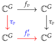
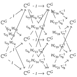
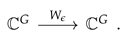
• For every $v\in \tilde{V}$, we have this commutative diagram:

where $\tilde{V}$ is a set of all vertices in the hidden layer. If for every $v\in V$, ${\tau }_v$is bijective, then τ is an isomorphism and $(W,f)$ is isomorphic to $(W^{\prime },f^{\prime })$ [4].

Now, we will see the similarity of neural network functions from two isomorphic neural networks.

Theorem 3.

If $(W,f)$ and $(V,g)$ are two isomorphic ${\mathbb{C}}^G$-neural networks then

$$\Psi (W,f)\left(x\right)=\Psi (V,g)\left(x\right).$$

Proof. 

Let $(W,f)$ and $(V,g)$ be two isomorphic ${\mathbb{C}}^G$-neural networks. It means that there is an isomorphism $\tau$ such that $\tau \diamond (W,f)=(V,g)$. Let $ϵ:s\left(ϵ\right)\to t\left(ϵ\right)$ be an arrow in Q. Let $x\in \left({\mathbb{C}}^G\right)d$ be an input vertex for $(W,f)$ and $(V,g)$. If v is an input vertex, we have

$$a{(W,f)}_v\left(x\right)=a{(V,g)}_v\left(x\right)=\left\{\begin{array}{cc}{x}_v\hfill & v\mathrm{is}\mathrm{an}\mathrm{input}\mathrm{vertex}\hfill \\ 1\hfill & v\mathrm{is}\mathrm{a}\mathrm{bias}\mathrm{vertex}\hfill \end{array}\right.$$

because ${\tau }_v=id$.

If v is in the first hidden layer, we have

$$\begin{array}{cc}\hfill a{(V,g)}_v\left(x\right)& =g_v\left(\sum _{ϵ\in {\zeta }_v}{V}_{ϵ}a{(V,g)}_{s\left(ϵ\right)}\left(x\right)\right)\hfill \\ \hfill & ={\tau }_v{f}_v\left({\tau }_v^{-1}\sum _{ϵ\in {\zeta }_v}{V}_{ϵ}a{(V,g)}_{s\left(ϵ\right)}\left(x\right)\right)\hfill \\ \hfill & ={\tau }_v{f}_v\left({\tau }_v^{-1}\sum _{ϵ\in {\zeta }_v}{\tau }_{t\left(ϵ\right)}{W}_{ϵ}{\tau }_{s\left(ϵ\right)}a{(V,g)}_{s\left(ϵ\right)}\left(x\right)\right)\hfill \\ \hfill & ={\tau }_v{f}_v\left(\sum _{ϵ\in {\zeta }_v}{\tau }_v^{-1}{\tau }_v{W}_{ϵ}a{(V,g)}_{s\left(ϵ\right)}\left(x\right)\right)\hfill & \hfill & \mathrm{because}{\tau }_{s\left(ϵ\right)}=1\hfill \\ \hfill & ={\tau }_v{f}_v\left(\sum _{ϵ\in {\zeta }_v}{W}_{ϵ}a{(V,g)}_{s\left(ϵ\right)}\left(x\right)\right).\hfill \end{array}$$

Since $s\left(ϵ\right)$ is an output vertex, then $a{(V,g)}_{s\left(ϵ\right)}\left(x\right)=a{(W,f)}_{s\left(ϵ\right)}\left(x\right)$. Hence, we get

$$a{(V,g)}_v\left(x\right)={\tau }_v{f}_v\left(\sum _{ϵ\in {\zeta }_v}{W}_{ϵ}a{(W,f)}_{s\left(ϵ\right)}\left(x\right)\right).$$

Therefore, we get

$$a{(V,g)}_v\left(x\right)={\tau }_{v}a{(W,f)}_v\left(x\right).$$

(2)

For v in the second hidden layer, we have

$$\begin{array}{cc}\hfill a{(V,g)}_v\left(x\right)& =g_v\left(\sum _{ϵ\in {\zeta }_v}{V}_{ϵ}a{(V,g)}_{s\left(ϵ\right)}\left(x\right)\right)\hfill \\ \hfill & ={\tau }_v{f}_v\left({\tau }_v^{-1}\sum _{ϵ\in {\zeta }_v}{V}_{ϵ}a{(V,g)}_{s\left(ϵ\right)}\left(x\right)\right)\hfill \\ \hfill & ={\tau }_v{f}_v\left({\tau }_v^{-1}\sum _{ϵ\in {\zeta }_v}{\tau }_{t\left(ϵ\right)}{W}_{ϵ}{\tau }_{s\left(ϵ\right)}^{-1}a{(V,g)}_{s\left(ϵ\right)}\left(x\right)\right)\hfill \\ \hfill & ={\tau }_v{f}_v\left(\sum _{ϵ\in {\zeta }_v}{\tau }_v^{-1}{\tau }_v{W}_{ϵ}{\tau }_{s\left(ϵ\right)}^{-1}{\tau }_{s\left(ϵ\right)}a{(W,f)}_{s\left(ϵ\right)}\left(x\right)\right)\hfill & \hfill & \mathrm{because}ϵ\in {\zeta }_v\hfill \\ \hfill & ={\tau }_v{f}_v\left(\sum _{ϵ\in {\zeta }_v}{W}_{ϵ}a{(W,f)}_{s\left(ϵ\right)}\left(x\right)\right)\hfill \\ \hfill & ={\tau }_{v}a{(W,f)}_v\left(x\right)\hfill & \hfill & \mathrm{from}\mathrm{the}\mathrm{definition}\mathrm{of}(W,f).\hfill \end{array}$$

It means if v is in the second hidden layer, we get

$$a{(V,g)}_v\left(x\right)={\tau }_{v}a{(W,f)}_v\left(x\right).$$

Inductively, we will get $a{(V,g)}_v\left(x\right)={\tau }_{v}a{(W,f)}_v\left(x\right)$ for every v in the hidden layer. If v is an output vertex, we have

$$\begin{array}{cc}\hfill a{(V,g)}_v\left(x\right)& =\sum _{ϵ\in {\zeta }_v}{V}_{ϵ}a{(V,g)}_{s\left(ϵ\right)}\left(x\right)\hfill \\ \hfill & =\sum _{ϵ\in {\zeta }_v}{\tau }_{t\left(ϵ\right)}{W}_{ϵ}{\tau }_{s\left(ϵ\right)}a{(V,g)}_{s\left(ϵ\right)}\left(x\right)\hfill \\ \hfill & =\sum _{ϵ\in {\zeta }_v}{\tau }_v{W}_{ϵ}{\tau }_{s\left(ϵ\right)}^{-1}{\tau }_{s\left(ϵ\right)}a{(W,f)}_{s\left(ϵ\right)}\left(x\right)\hfill & \hfill & \mathrm{because}s\left(ϵ\right)\mathrm{is}\mathrm{in}\mathrm{hidden}\mathrm{layer}\hfill \\ \hfill & =\sum _{ϵ\in {\zeta }_v}{W}_{ϵ}a{(W,f)}_{s\left(ϵ\right)}\left(x\right)\hfill & \hfill & \mathrm{because}{\tau }_v=1\mathrm{for}v\in V^{\prime }.\hfill \end{array}$$

Therefore, we get

$$a{(V,g)}_v\left(x\right)=a{(W,f)}_v\left(x\right).$$

It means for every output vertex v we get

$$\Psi (W,f)=\Psi (V,g).$$

□

3.2. Moduli Spaces of Neural Network

The last theorem tells us two isomorphic neural networks will have the same neural network function. The moduli spaces can be defined by the isomorphic classes of neural networks as follows.

Definition 16.

Let G be a group and X be a set. An action of G on X is a map $·:G\times X\to X$, denoted by $a·x$ such that

• $e·x=x$ for every $x\in X$ where e is the identity in G,
• $a·(b·x)=(a·b)·x$ for all $a,b\in G$ and all $x\in X$.

The set $\mathcal{O}=\left\{a·x|a\in G\right\}$ is called an orbit of the action [8].

We know that $\Gamma \left(Q\right)$ is a group of isomorphisms. Let ${}^G\left(Q\right)$ be a set of all ${\mathbb{C}}^G$-representation of Q. Define a map

$$\begin{array}{cc}\hfill ·:& \Gamma \left(Q\right)\times {\mathbb{C}}^G\left(Q\right)\to {\mathbb{C}}^G\left(Q\right)\hfill \\ \hfill & (\tau ·W)\mapsto \tau ·W.\hfill \end{array}$$

where $\tau ·W=\tau W{\tau }^{-1}$. We know that the map · is an action of $\Gamma \left(Q\right)$ on ${\mathbb{C}}^G\left(Q\right)$ because we have $I={\left\{i{d}_{{}^G}\right\}}_{v\in V}\in \Gamma \left(Q\right)$ and $IW{I}^{-1}=IWI=W$ for all $W\in {\mathbb{C}}^G\left(Q\right)$. We also have

$$\tau ·(\sigma ·W)=\tau ·\left(\sigma W{\sigma }^{-1}\right)=\tau \sigma W{\sigma }^{-1}\tau -1=\left(\tau \sigma \right)W{\left(\tau \sigma \right)}^{-1}=(\tau ·\sigma )·W$$

for all $\tau ,\sigma \in \Gamma \left(Q\right)$ and all $W\in {\mathbb{C}}^G\left(Q\right)$. Now, we can define $M\left(Q\right)$ as the set of all orbits of the action of $\Gamma$ on ${\mathbb{C}}^G\left(Q\right)$. The set $M\left(Q\right)$ is the moduli space of ${\mathbb{C}}^G$-representations (see also [9]). We will apply the same group action to ${\mathbb{C}}^G\left(Q\right)$ as a subgroup of $\Gamma \left(Q\right)$ and ${\mathcal{C}}_{{\mathbb{C}}^G}\left(Q\right)$ as a subset of ${\mathbb{C}}^G\left(Q\right)$. We know that the map · is also a group action of ${\mathcal{C}}_{\Gamma }\left(Q\right)$ on ${\mathcal{C}}_{{\mathbb{C}}^G}\left(Q\right)$.

Definition 17.

Let $Q=(V,E,s,t)$ be a network quiver. Define an action of ${\mathcal{C}}_{\Gamma }\left(Q\right)$ on ${\mathcal{C}}_{{\mathbb{C}}^G}\left(Q\right)$ as $\tau ·W=\tau W{\tau }^{-1}$. The moduli space $\mathcal{M}\left(Q\right)$ of the convolution representation is the set of all orbits from the group action.

Let $\tilde{W}$ be a convolution representation of $\tilde{Q}$. We can fix a family of vector spaces ${\left\{U_v\right\}}_{v\in \tilde{V}}$ indexed by $v\in \tilde{V}$ and given $V_v={\left({\mathbb{C}}^G\right)}^k$ if v is an output vertex in $\tilde{Q}$ and $V_v=0$ for any other vertices in $\tilde{Q}$. A choice of convolution representations $\tilde{W}$ of hidden quiver $\tilde{Q}$ and a linear map $h_v:{\tilde{W}}_v\to V_v$ for each $v\in \tilde{V}$ determines a pair $(\tilde{W},h)$ where $h={\left\{h_v\right\}}_{v\in \tilde{V}}$ that is known as a framed quiver representation of $\tilde{Q}$ by the family of vector spaces ${\left\{V_v\right\}}_{v\in \tilde{V}}$. From the definition, we can say $ker\left(h\right)={\left\{ker{\left(h\right)}_v\right\}}_{v\in \tilde{V}}$.

Dually, we can fix a family of vector spaces ${\left\{U_v\right\}}_{v\in \tilde{V}}$ indexed by $v\in \tilde{V}$ and given $U_v={\left({\mathbb{C}}^G\right)}^d$ when v is an input vertex of $\tilde{Q}$ and $U_v=0$ for any other $v\in \tilde{V}$. A choices of convolution representation $\tilde{W}$ of hidden quiver $\tilde{Q}$ and a linear map $l_v:U_v\to \tilde{W}$ for each $v\in \tilde{V}$ determines a pair $(l,\tilde{W})$ where $l={\left\{l_v\right\}}_{v\in \tilde{V}}$, that is known as co-framed quiver representation of $\tilde{Q}$ by the family of vector spaces ${\left\{U_v\right\}}_{v\in \tilde{V}}$. From the definition we can say $Im\left(l\right)={\left\{Im{\left(l\right)}_v\right\}}_{v\in \tilde{V}}$.

Definition 18.

A double-framed convolution quiver representation is a triple $(l,\tilde{W},h)$ where $\tilde{W}$ is a convolution representation of quiver $\tilde{Q}$, $(\tilde{W},h)$ is a framed quiver representation of $\tilde{Q}$, and $(l,\tilde{W})$ is a co-framed quiver representation of $\tilde{Q}$ [4].

Now, we will see the stability of the double-framed moduli space.

Definition 19.

A double-framed quiver representation $(l,\tilde{W},h)$ is stable if

• The subrepresentation that contained in $ker\left(h\right)$ is only zero sub representation;
• The subrepresentation that contains $Im\left(l\right)$ is only $\tilde{W}$ [4].

From this definition, we can get this lemma.

Lemma 3.

Let $(l,\tilde{W},h)$ be a double-framed convolution representation. We say $(l,\tilde{W},h)$ is stable if

• For every output vertex v, $ker\left(h_v\right)={\bigcap }_{i=1}^{k}ker({\left(h_v\right)}_i$ holds;
• For every input vertex v, $Im\left(l_v\right)=span({\bigcup }_{i=1}^{k}Im\left({\left(l_v\right)}_i\right)$ holds.

This lemma only gives us a sufficient condition for the stability condition. Not all double-framed convolution representations are stable. Nevertheless, we can see the dimension of the moduli space. Let us see this example first.

Example 1.

Let Q be a network quiver that is drawn like this:

We can make the delooped quiver from Q as $Q°$

After that, we will make a new quiver as follows:

The quiver will be denoted as $Q^v$. The ${\mathbb{C}}^G$ quiver representation of Q is as follows:

We can also choose a morphism of representation τ such that ${\tau }_{a_3}={W_{{ϵ}_1}}^{-1}$, ${\tau }_{a_4}=W_{{ϵ}_5}^{-1}$, ${\tau }_{a_5}=W_{{ϵ}_6}^{-1}$, ${\tau }_{a_6}={W_{{ϵ}_1}}^{-1}{\tau }_{W_{{ϵ}_7}}^{-1}$, ${\tau }_{a_7}={W_{{ϵ}_5}}^{-1}{W_{{ϵ}_{11}}}^{-1}$, ${\tau }_{a_8}={W_{{ϵ}_6}}^{-1}{W_{{ϵ}_{15}}}^{-1}$, and ${\tau }_{a_1}={\tau }_{a_2}={\tau }_{a_9}={\tau }_{a_{1}0}=I$ such that quiver $Q^V$ has weight equal to identity for all arrows:

So, we will get that the dimension of double-framed convolution representation is proportioned by the number of arrows that are not equal to identity.

Theorem 4.

Let $V_{in}$ be the set of input vertices of Q and $V_{out}$ be the set of output vertices from Q. Define

$${\mathcal{C}}_{\Gamma }\left(\tilde{Q}\right)={\left\{I\right\}}_{v\in V_{in}}\times \prod _{v\in \tilde{V}}Cir\left({\mathbb{C}}^G\right)\times {\left\{I\right\}}_{v\in V_{out}}.$$

Let $\mathcal{M}\left(\tilde{Q}\right)$ be the set of all orbits from the action of ${\mathcal{C}}_{\Gamma }\left(\tilde{Q}\right)$ on ${\mathcal{C}}_{{}^G}\left(\tilde{Q}\right)$, then the set $\mathcal{M}\left(\tilde{Q}\right)$ will form the moduli space. Furthermore, the dimension of the moduli space is $\left|G\right|\left(\right|E°|-|\tilde{V}\left|\right)$.

Proof. 

Let Q be a network quiver with $\tilde{Q}$ as the hidden quiver and $Q°$ as the delooped quiver. Let W be a convolution representation of quiver $Q°$. Let $v\in \tilde{V}$. We know that there is $ϵ\in E°$ such that $t\left(ϵ\right)=v$. We only choose one $ϵ\in E°$ that $t\left(ϵ\right)=v$ for every $v\in \tilde{V}$ to build a new quiver $Q^v$. Because of the construction, no two arrows have the same target. This implies that $Q^v$ is a union of trees, and the intersection of any two trees can only be a source vertex of Q. Furthermore, for any of those trees, only a vertex that is hidden is a unique source corresponding to that tree. Now, we will construct a morphism of quiver representations $\tau ={\left\{{\tau }_v\right\}}_{\{v\in V\}}$. If v is the input vertex, set the ${\tau }_v=1$. If v is not the input vertex, we have an arrow $\alpha \in Q^v$ such that $t\left(\alpha \right)=v$. So, we can set ${\tau }_v=W_{\alpha }^{-1}{\tau }_{s\left(\alpha \right)}$. Using the recursive formula, we can get a new convolution representation of $Q^v$ such that every arrow in $Q^v$ will be represented as identity linear maps from ${\mathbb{C}}^G$ to ${\mathbb{C}}^G$. From that fact, we can conclude that the number of free choices of quiver representation will be the same as the number of arrows in $Q°$ that have not been set to identity. Consider

Using Fourier transformation, we know the dimension of $C=\{T:{\mathbb{C}}^G\to {\mathbb{C}}^G|\exists a\in {\mathbb{C}}^G\ni T\left(f\right)=a\ast f\}$ is equal to $\left|G\right|$. Therefore, the dimension of the moduli space is $\left|G\right|\left(\right|E°|-|\tilde{V}\left|\right)$. □

4. Conclusions

We have defined a neural network function from an artificial neural network formed by ${\mathbb{C}}^G$ representation, especially for convolution representation. We can also see some moduli space properties formed by the action of the isomorphism group on the set of all convolution representations. From this work, we can minimize the complexity of the neural network algorithm.

In further research, we will explore the moduli spaces from recurrent neural networks and the topology of moduli spaces. We will see some properties of neural network functions with some types of activation functions and their effect on the continuity of neural network functions.

References

- Zhang, Q.; Wang, Y. Construction of composite mode of sports education professional football teaching based on sports video recognition technology. In Proceedings of the 2020 5th International Conference on Mechanical, Control and Computer Engineering (ICMCCE), Harbin, China, 25–27 December 2020; Volume 5, pp. 1889–1893. [Google Scholar]
- Schöller, F.E.T.; Blanke, M.; Plenge-Feidenhans, M.K.; Nalpantidis, L. Vision-based Object Tracking in Marine Environments using Features from Neural Network Detections. IFAC-PapersOnLine 2020, 52, 14517–14523. [Google Scholar] [CrossRef]
- Belov-Kanel, A.; Rowen, L.H.; Vishne, U. Application of Full Quivers of Representations of Algebras, to Polynomial Identities. Commun. Algebra 2011, 39, 4536–4551. [Google Scholar] [CrossRef]
- Armenta, M.; Jodoin, P.-M. The Representation Theory of Neural Networks. Mathematics 2021, 9, 3216. [Google Scholar] [CrossRef]
- Armenta, M.; Judge, T.; Painchaud, N.; Skandarani, Y.; Lemaire, C.; Gibeau Sanchez, G.; Spino, P.; Jodoin, P.-M. Neural Teleportation. Mathematics 2023, 11, 480. [Google Scholar] [CrossRef]
- Assem, I.; Simson, D.; Skowronski, A. Quivers and Algebras. In Elements of the Representation Theory of Associative Algebras; CUP: New York, NY, USA, 2007; Volume 1, pp. 41–96. [Google Scholar]
- Wanditra, L.C.; Muchtadi Alamsyah, I.; Rachmaputri, G. Wave Packet Transform on Finite Abelian Group. Southeast Asian Bull. Math. 2020, 44, 843–857. [Google Scholar]
- Isaacs, I.M. Quivers and Algebras. In Algebra; Graduate Studies in Mathematics; American Mathematical Society: New York, NY, USA, 2009; pp. 42–54. [Google Scholar]
- Armenta, M.; Brüstle, T.; Hassoun, S.; Reineke, M. Double framed moduli spaces of quiver representations. Linear Algebra Its Appl. 2022, 650, 98–131. [Google Scholar] [CrossRef]
Disclaimer/Publisher’s Note: The statements, opinions and data contained in all publications are solely those of the individual author(s) and contributor(s) and not of MDPI and/or the editor(s). MDPI and/or the editor(s) disclaim responsibility for any injury to people or property resulting from any ideas, methods, instructions or products referred to in the content. |
© 2023 by the authors. Licensee MDPI, Basel, Switzerland. This article is an open access article distributed under the terms and conditions of the Creative Commons Attribution (CC BY) license (https://creativecommons.org/licenses/by/4.0/).
Share and Cite
Wanditra, L.C.; Muchtadi-Alamsyah, I.; Nasution, D. Artificial Neural Networks Using Quiver Representations of Finite Cyclic Groups. Symmetry 2023, 15, 2110. https://doi.org/10.3390/sym15122110
Wanditra LC, Muchtadi-Alamsyah I, Nasution D. Artificial Neural Networks Using Quiver Representations of Finite Cyclic Groups. Symmetry. 2023; 15(12):2110. https://doi.org/10.3390/sym15122110
Chicago/Turabian StyleWanditra, Lucky Cahya, Intan Muchtadi-Alamsyah, and Dellavitha Nasution. 2023. "Artificial Neural Networks Using Quiver Representations of Finite Cyclic Groups" Symmetry 15, no. 12: 2110. https://doi.org/10.3390/sym15122110
APA StyleWanditra, L. C., Muchtadi-Alamsyah, I., & Nasution, D. (2023). Artificial Neural Networks Using Quiver Representations of Finite Cyclic Groups. Symmetry, 15(12), 2110. https://doi.org/10.3390/sym15122110