Multiplicity Dependence of the Freeze-Out Parameters in Symmetric and Asymmetric Nuclear Collisions at Large Hadron Collider Energies

Abstract

Strange hadron transverse momentum spectra are analyzed in symmetric $pp$ and $PbPb$ and asymmetric $pPb$ collision systems for their dependence on rapidity and event charged-particle multiplicity. The thermodynamically consistent Tsallis models with and without flow velocity are used to reproduce the experimental data, extracting the freeze-out parameters to gain insights into the underlying physics of the collision processes by looking into the parameters change with different multiplicities, particle types, and collision geometries. We found that with an increase in the event multiplicity, the average transverse flow velocity, effective, and kinetic freezeout temperatures increase, with heavier strange particle species exhibiting a more significant increase. The value of the non-extensivity parameter decreases with an increase in the multiplicity of the particles. For heavier particles, larger $T_{eff}$ and $T_0$ and smaller q have been observed, confirming the quick thermalization and equilibrium for massive particles. Furthermore, the differences in parameter values for particle species are more significant in $pp$ and $pPb$ collisions than in $PbPb$ collisions. In addition, in symmetric $pp$ and $PbPb$ collisions, parameter values ($q,T_0,{\beta }_T$) show more significant shifts for heavier particles compared to the lighter ones. In contrast, in asymmetric $pPb$ collisions, both heavier and lighter particles display uniform linear progression.

1. Introduction

Studies of strange particles produced in high-energy collisions of hadrons and heavy ions provide insight into the dynamics of collision processes. Previous measurements reported by the RHIC at BNL and SPS at CERN demonstrated increased strangeness production compared to proton–proton collisions [1,2]. This phenomenon is believed to be attributed to the creation of a quark–gluon medium with high energy density [3]. The observed quantities of strange particles at various center-of-mass energies are well reproduced by thermal statistical models [4,5,6,7]. In RHIC’s gold–gold (AuAu) collisions, notable correlations were detected in the azimuthal direction among the final-state hadrons, which suggests the creation of a medium that exhibits characteristics akin to those of a nearly perfect fluid undergoing an anisotropic expansion driven by pressure [2]. Similarly, investigations of the production and behavior of strange and light-flavored particles in heavy-ion collisions have yielded a deeper understanding of the fluid-like nature of the medium, which shows the collective behavior of the medium at the partonic level [2,8].

In this paper, we provide analyses of strange-particle spectra in $pp$, $pPb$, and $PbPb$ collisions taken from [9], observing their variation with event multiplicity. We focus on the spectra of $K_S^0$, $\mathrm{\Lambda }$, and $\mathrm{\Xi }$ particles, considering the charge-conjugate states for $\mathrm{\Xi }$ and $\mathrm{\Lambda }$ particles. For the analyses, we applied both the thermodynamically consistent Tsallis distribution functions (with and without the transverse flow velocity)to extract parameters pertinent to the collective characteristics of nuclear matter. The extensive utilization of the Tsallis distribution function [10,11,12,13] within high-energy proton–proton collisions finds justification in its remarkably effective description of experimental $p_T$ spectra for hadrons. This is achieved using a minimal set of parameters: the first being the effective temperature ($T_{eff}$), the second being the non-extensivity parameter (q), which captures deviations from the Boltzmann–Gibbs exponential distribution, and the third parameter being the fitting constant, proportionally associated with system volume. In contrast to other statistical distributions, the Tsallis distribution function stands out due to its distinctive advantage: a direct link to thermodynamics through entropy [14]. The non-extensivity index (q) of the Tsallis function holds significant relevance in quantifying the extent of departure of the particle’s transverse momentum distribution from the exponential Boltzmann–Gibbs distribution. Importantly, the parameter q also acts as an indicator of non-equilibrium or the degree of non-thermalization within a system [15]. Its significance within non-extensive statistical mechanics is reaffirmed by recent work [16] conducted by Tsallis. This underscores the intrinsic value of the q parameter and its pivotal role in understanding system dynamics and deviations from traditional statistical behavior.

Several adaptations of the Tsallis function have been equally successful in accurately characterizing the $p_T$ distributions of end-state hadrons in proton–proton collisions, encompassing the entire range of available $p_T$ values observed in experiments at both the Relativistic Heavy Ion Collider (RHIC) and the Large Hadron Collider (LHC) [17,18,19,20]. Various transverse flow models have been integrated with Tsallis statistics to elucidate the $p_T$ distributions of hadrons in nuclear collisions at both RHIC and LHC [21,22,23,24,25,26,27,28]. We employed the Tsallis formula with and without an intrinsic flow velocity to deduce the kinetic freeze-out temperature, transverse expansion velocity, and non-extensive parameter [13,24,25,29].

2. The Method and Formalism

In this study, we conducted an analysis of experimental data gathered by the CMS collaboration [9] from collisions involving $pp$, $pPb$, and $PbPb$ at energies of 7, 5.02, and 2.76 TeV, respectively. The track selection was established based on the specific kinematic criteria of |$\eta$| < 2.4 and $p_T$> 0.4 GeV/c [30,31]. These criteria were chosen to ensure the precision and reliability of the track selection process. In the source paper [9], data from pp, pPb, and PbPb collisions were sorted using $N_{trk}^{offline}$, representing the number of offline reconstructed tracks. Correction for detector and algorithm inefficiencies was performed within the kinematic region ($\left|\eta \right|<2.4$ and $p_T>0.4$ GeV) denoted by $N_{trk}^{corrected}$. The analysis determined fractions of total multiplicity within $N_{trk}^{offline}$ intervals and tracked the average number of corrected tracks. The tracking efficiency uncertainty was 3.9% for single tracks [32]. For pp data, six multiplicity intervals were created, inclusive for lower bounds, matching $N_{trk}^{offline}<35$ for minimum-bias events. PbPb and pPb data featured eight intervals, with pPb’s $N_{trk}^{offline}$ not in the center-of-mass frame. In the latter case, when using the CMS frame, an insignificant difference is disregarded. Detector stability was confirmed across various multiplicities [9]. To gain insights into the collective characteristics of strongly interacting matter, we employed the thermodynamically consistent simple Tsallis distribution function, and the one incorporating a definition for flow velocity. These functions were utilized to extract parameters that offer insights into the overall properties of the strongly interacting medium. The following simple form of the Tsallis distribution function is used to fit the data.

$$\frac{1}{N_{ev}}\frac{1}{2\pi p_T}\frac{d^{2}N}{dyd{p}_T}=C{m}_T{\left(1+(q-1)\frac{m_T}{T_{eff}}\right)}^{-q/(q-1)}$$

(1)

Here, $m_T$ is the transverse mass which is given by $m_T=\sqrt{p_T^2+m_0^2}$ where $p_T$ and $m_0$ are the transverse momentum and rest mass of the observed particle, respectively, $T_{eff}$ (Effective Temperature) reflects the average thermal motion of particles within the system. It governs how particles are distributed in terms of their transverse momentum. A higher $T_{eff}$ generally corresponds to particles with higher transverse momenta and more energy. The q is the non-extensivity parameter that characterizes deviations from the standard Boltzmann–Gibbs distribution. A value of q close to 1 indicates a distribution resembling the conventional exponential distribution, while q values different from 1 signify non-extensive effects that might arise from complex interactions or correlations among particles. The symbol C is used to reflect the Normalization Constant that ensures that the probability density integrates to unity over the entire range of possible values. It helps scale the distribution function appropriately to match the experimental data.

Likewise, transverse flow is introduced into the Tsallis function given above through a transformation involving the replacement of the term $m_T$ with $<m_T>(m_T-p_T<{\beta }_T>)$ [33]. This manipulation results in a functional form of the Tsallis distribution function given below.

$$\begin{array}{c}\hfill \frac{1}{N_{ev}}\frac{1}{2\pi p_T}\frac{d^{2}N}{dyd{p}_T}=C<{\gamma }_T>\left(m_T-p_T<{\beta }_T>\right)\\ \hfill \times {\left(1+<{\gamma }_T>\frac{(q-1)(m_T-p_T<{\beta }_T>)}{T_0}\right)}^{-q/(q-1)}\end{array}$$

(2)

The parameters used in the function are: $<{\gamma }_T>$ is the Average Boost Factor given by $<{\gamma }_T>$ = $1/\sqrt{1-{\beta }_T^2}$, $<{\beta }_T>$ is the average flow velocity that signifies the average speed at which particles collectively flow, $T_0$ is the kinetic freeze-out Temperature denoting the temperature at which particles cease interactions resulting in the transverse momentum $p_T$ of the particle constant, and q is the non-extensivity parameter defined above. The function was originally derived in Ref. [33] and utilized in Refs. [33,34], to study final particles within high-energy heavy-ion and proton–proton collisions. To achieve this, a straightforward Lorentz transformation was employed, facilitating the inclusion of transverse expansion velocity into the simple and thermodynamically consistent Tsallis functions. This approach proved successful in examining the centrality dependence of the $p_T$ distributions of identified hadrons in Xe + Xe collisions at a collision energy of $\sqrt{s_{NN}}$ = 5.44 TeV [33] and PbPb collisions at 5.02 TeV [34]. These specific distributions were initially recorded by the ALICE Collaboration and documented in Refs. [35,36].

3. Results and Discussion

In this section, we present the analyses of the transverse momentum spectra of strange hadrons through the application of Tsallis statistics. The strange particles $K_S^0$, $\mathrm{\Lambda }$, and $\mathrm{\Xi }$ are investigated using diverse collision scenarios, including $pp$, $pPb$, and $PbPb$ collisions, each occurring at energies of 7, 5.02, and 2.76 TeV, respectively. The production of strange particles in high multiplicity pp events is one of the signatures of the existence of the parton dominant medium, i.e., QGP. Therefore, it is important to analyze the strange particles to have an insight into the strongly interacting matter. The data employed for these analyses were collected using the advanced CMS detector situated at the CERN Large Hadron Collider (LHC).

The $p_T$ distributions of the particles are studied in several event-based charged-particle multiplicities. The research explores freeze-out parameters in relation to particle species and event multiplicity. The study aimed to understand how particles freezeout and how this process is connected to the produced particles in various collisions. In Figure 1, Figure 2 and Figure 3, we applied scaling to the data and performed the line fitting using a scaling factor defined as scale_factor = scale_factor × N. The initial scale factor was set to 10, and ’N’ is an integer starting from 1. As a result, the data were scaled by factors such as 10, 20, 60, 240, and so forth. This approach was adopted to improve the clarity of visualizing the fit results and to prevent data overlap. Figure 1, Figure 2 and Figure 3 depict $p_T$ distributions of charged particles categorized by various multiplicity classes. The geometric symbols represent experimental data, while solid and dashed lines indicate fits generated by the Tsallis without and with flow, respectively. Figure 1 shows $p_T$ distributions of $K_S^0$, $\mathrm{\Lambda }$, and $\mathrm{\Xi }$ in 7 TeV $pp$ collisions; Figure 2 illustrates the same for $pPb$ collisions at 5.02 TeV; and Figure 3 portrays the scenario in $PbPb$ collisions at 2.76 TeV. The overlaid lines demonstrate an excellent fit of both functions to the data. Beneath each plot, a ratio of data to fit is presented, indicating the accuracy of the function’s representation. While the solid and dashed lines distinguish the two equations in the graphs, the distinction is marked by full and hollow geometric symbols in the ratio graphs. Solid symbols represent the Tsallis function (given as Equation (1)), while hollow symbols signify the function given as Equation (2). The results obtained from the fitting procedure using Equations (1) and (2) are tabulated in six separate tables. Table 1, Table 2 and Table 3 provide fitting results for Figure 1, Figure 2 and Figure 3, respectively, using the Tsallis function (Equation (1)). Correspondingly, Table 4, Table 5 and Table 6 present fitting outcomes for the same figures using Equation (2).

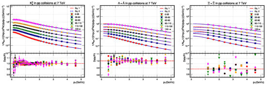
Figure 1. The graphical representation displays the fit function outcomes depicted as lines superimposed on the experimental data, visualized using colored symbols. These observations pertain to strange particles distributed across various multiplicity classes and obtained from proton–proton ($pp$) collisions at an energy of 7 TeV [9]. Specifically, the solid line corresponds to the outcomes derived from the fit function defined in Equation (1), while the dashed line corresponds to the outcomes yielded by the fit function outlined in Equation (2). The fits are performed utilizing partial measurements with |$\eta$| < 2.4 and $p_T$> 0.4 GeV/c. The lower section of each figure shows the data-to-fit ratio, which serves as an indicator of the fit’s quality. Within this ratio plot, filled symbols represent the outcomes of the fit based on Equation (1) in relation to the data, whereas hollow symbols signify the outcomes of the fit utilizing Equation (2) in relation to the data.

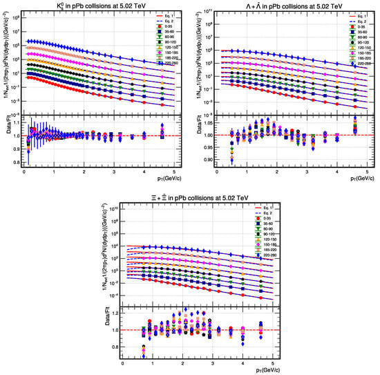
Figure 2. The graphical representation displays the fit function outcomes depicted as lines superimposed on the experimental data, visualized using colored symbols. These observations pertain to strange particles distributed across various multiplicity classes and obtained from proton–lead ($pPb$) collisions at an energy of 5.02 TeV [9]. Specifically, the solid line corresponds to the outcomes derived from the fit function defined in Equation (1), while the dashed line corresponds to the outcomes yielded by the fit function outlined in Equation (2). The fits are performed utilizing partial measurements with |$\eta$| < 2.4 and $p_T$> 0.4 GeV/c. The lower section of each figure shows the data-to-fit ratio, which serves as an indicator of the fit’s quality. Within this ratio plot, filled symbols represent the outcomes of the fit based on Equation (1) in relation to the data, whereas hollow symbols signify the outcomes of the fit utilizing Equation (2) in relation to the data.

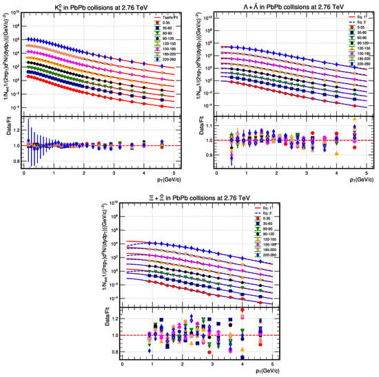
Figure 3. The graphical representation displays the fit function outcomes depicted as lines superimposed on the experimental data, visualized using colored symbols. These observations pertain to strange particles distributed across various multiplicity classes and obtained from lead–lead ($PbPb$) collisions at an energy of 2.76 TeV [9]. Specifically, the solid line corresponds to the outcomes derived from the fit function defined in Equation (1), while the dashed line corresponds to the outcomes yielded by the fit function outlined in Equation (2). The fits are performed utilizing partial measurements with |$\eta$| < 2.4 and $p_T$> 0.4 GeV/c. The lower section of each figure shows the data-to-fit ratio, which serves as an indicator of the fit’s quality. Within this ratio plot, filled symbols represent the outcomes of the fit based on Equation (1) in relation to the data, whereas hollow symbols signify the outcomes of the fit utilizing Equation (2) in relation to the data.

Table 1. Freeze-out parameter extracted from the fit procedure on experimental data [9] for $K_S^0$, $\mathrm{\Lambda }$, and $\mathrm{\Xi }$ in $pp$ collisions at 7 TeV with the fit function given in Equation (1).

Particle	Mult.	${\mathit{T}}_{\mathit{eff}}$ (GeV/c)	q	C	${\mathit{\chi }}^2$	$\mathit{ndof}$
	0–35	0.09816 ± 0.00128	1.15244 ± 0.00099	40.20290 ± 2.00218	1.15170	25
	35–60	0.14767 ± 0.00112	1.14342 ± 0.00083	25.27069 ± 0.64541	0.56557	25
$K_S^0$	60–90	0.17642 ± 0.00217	1.13986 ± 0.00158	18.09327 ± 0.70491	1.47367	25
$pp$	90–110	0.20807 ± 0.00429	1.13130 ± 0.00307	14.27054 ± 0.87777	5.17861	25
7 TeV	110–130	0.22167 ± 0.00368	1.13071 ± 0.00262	13.14619 ± 0.63434	3.45691	25
	130–∞	0.23760 ± 0.00541	1.12904 ± 0.00381	11.61978 ± 0.75382	6.30689	25
	0–35	0.12185 ± 0.00547	1.10901 ± 0.00261	67.57438 ± 14.93095	1.55954	14
	35–60	0.24379 ± 0.00503	1.08185 ± 0.00233	8.25738 ± 0.66556	0.75211	14
$\mathrm{\Lambda }+\overline{\mathrm{\Lambda }}$	60–90	0.31297 ± 0.01090	1.06923 ± 0.00497	4.03398 ± 0.49937	2.20260	14
$pp$	90–110	0.41362 ± 0.01531	1.04504 ± 0.00684	1.96147 ± 0.23214	3.66630	14
7 TeV	110–130	0.44500 ± 0.01968	1.04290 ± 0.00884	1.67442 ± 0.22677	4.97901	14
	130–∞	0.47042 ± 0.01648	1.03890 ± 0.00729	1.56011 ± 0.16516	2.83025	14
	0–35	0.14474 ± 0.03052	1.10333 ± 0.01199	4.58444 ± 4.93836	1.02112	6
	35–60	0.27596 ± 0.02425	1.07055 ± 0.00952	0.90585 ± 0.44000	2.6662	6
$\mathrm{\Xi }+\overline{\mathrm{\Xi }}$	60–90	0.34538 ± 0.09520	1.0557 ± 0.03937	0.45905 ± 0.0724	4.3445	6
$pp$	90–110	0.53090 ± 0.05117	1.02418 ± 0.01925	0.11338 ± 0.03536	0.80319	6
7 TeV	110–130	0.54760 ± 0.05179	1.02287 ± 0.01983	0.11934 ± 0.03549	0.81505	6
	130–∞	0.55205 ± 0.07805	1.0199 ± 0.03039	0.13738 ± 0.06348	3.68301	6

Table 2. Freeze-out parameter extracted from the fit procedure on experimental data [9] for $K_S^0$, $\mathrm{\Lambda }$, and $\mathrm{\Xi }$ in $pPb$ collisions at 5.02 TeV with the fit function given in Equation (1).

Particle	Multi.	${\mathit{T}}_{\mathit{eff}}$ (GeV/c)	q	C	${\mathit{\chi }}^2$	$\mathit{ndof}$
	0–35	0.11641 ± 0.00150	1.14201 ± 0.00114	26.50584 ± 1.25312	1.40998	25
	35–60	0.15136 ± 0.00129	1.13314 ± 0.00094	24.29349 ± 0.69950	0.79333	25
$K_S^0$	60–90	0.17255 ± 0.00147	1.12616 ± 0.00106	22.73868 ± 0.63223	0.91968	25
$pPb$	90–120	0.18774 ± 0.00169	1.12074 ± 0.00120	22.97426 ± 0.65810	1.10686	25
5.02 TeV	120–150	0.20263 ± 0.00217	1.11446 ± 0.00152	21.21529 ± 0.70591	1.74373	25
	150–185	0.21415 ± 0.00270	1.10922 ± 0.00187	20.49728 ± 0.79215	2.57615	25
	185–220	0.22551 ± 0.00329	1.10487 ± 0.00226	19.84267 ± 0.87372	3.66680	25
	220–260	0.23375 ± 0.00365	1.10004 ± 0.00249	20.00286 ± 0.93772	4.46033	25
	0–35	0.15943 ± 0.00303	1.09423 ± 0.00144	23.10003 ± 2.01989	0.43027	14
	35–60	0.26104 ± 0.00485	1.06850 ± 0.00222	6.29745 ± 0.45623	0.76934	14
	60–90	0.31750 ± 0.00729	1.05555 ± 0.00329	4.18432 ± 0.34717	1.41758	14
$\mathrm{\Lambda }+\overline{\mathrm{\Lambda }}$	90–120	0.37058 ± 0.00928	1.04056 ± 0.00412	3.13811 ± 0.26934	1.99797	14
$pPb$	120–150	0.40355 ± 0.00982	1.03270 ± 0.00433	2.73724 ± 0.22075	2.08080	14
5.02 TeV	150–185	0.43193 ± 0.01276	1.02479 ± 0.00558	2.46909 ± 0.23587	3.32342	14
	185–220	0.46165 ± 0.01354	1.01715 ± 0.00588	2.24793 ± 0.20796	3.47132	14
	220–260	0.48056 ± 0.01473	1.01034 ± 0.00635	2.21437 ± 0.21183	4.03902	14
	0–35	0.20413 ± 0.01664	1.07876 ± 0.00714	1.55049 ± 0.57371	1.89588	13
	35–60	0.32748 ± 0.01604	1.05114 ± 0.00671	0.49918 ± 0.09293	1.25786	13
	60–90	0.44485 ± 0.01626	1.01587 ± 0.00654	0.23903 ± 0.03021	1.11461	13
$\mathrm{\Xi }+\overline{\mathrm{\Xi }}$	90–120	0.51076 ± 0.03303	1.01154 ± 0.01301	0.18726 ± 0.03980	4.06315	13
$pPb$	120–150	0.53344 ± 0.04025	1.00579 ± 0.01611	0.19584 ± 0.04629	5.69623	13
5.02 TeV	150–185	0.55165 ± 0.00324	1.00283 ± 0.00378	0.20042 ± 0.00841	7.08035	13
	185–220	0.57872 ± 0.00000	1.00108 ± 0.00028	0.18537 ± 0.00703	11.80581	13
	220–260	0.58911 ± 0.05250	1.00048 ± 0.02086	0.19240 ± 0.05261	16.05159	13

Table 3. Freeze-out parameter extracted from the fit procedure on experimental data [9] for $K_S^0$, $\mathrm{\Lambda }$, and $\mathrm{\Xi }$ in $PbPb$ collisions at 2.76 TeV with the fit function given in Equation (1).

Particle	Multi.	${\mathit{T}}_{\mathit{eff}}$ (GeV/c)	q	C	${\mathit{\chi }}^2$	$\mathit{ndof}$
	0–35	0.09329 ± 0.00108	1.13940 ± 0.00084	79.94100 ± 3.73468	1.10688	25
	35–60	0.11231 ± 0.00088	1.13510 ± 0.00067	110.29351 ± 3.29644	0.62700	25
	60–90	0.12027 ± 0.00118	1.13089 ± 0.00092	133.52572 ± 4.85411	0.98610	25
$K_S^0$	90–120	0.12727 ± 0.00163	1.12654 ± 0.00121	150.56144 ± 7.10797	2.03220	25
$PbPb$	120–150	0.13869 ± 0.00193	1.11909 ± 0.00141	139.63669 ± 7.08373	2.85833	25
2.76 TeV	150–185	0.14657 ± 0.00255	1.11368 ± 0.00184	139.70330 ± 8.76329	4.92728	25
	185–220	0.15239 ± 0.00301	1.11066 ± 0.00216	142.42572 ± 10.03561	6.69866	25
	220–260	0.16127 ± 0.00364	1.10521 ± 0.00258	134.22032 ± 10.69523	9.76880	25
	0–35	0.11688 ± 0.00374	1.09731 ± 0.00182	140.66656 ± 23.39859	0.94394	14
	35–60	0.16609 ± 0.00350	1.08694 ± 0.00166	68.54274 ± 6.68959	0.65705	14
	60–90	0.18277 ± 0.00532	1.08279 ± 0.00251	67.60518 ± 8.82441	1.44519	14
$\mathrm{\Lambda }+\overline{\mathrm{\Lambda }}$	90-120	0.21310 ± 0.00555	1.07004 ± 0.00256	48.08948 ± 5.43211	1.58931	14
$PbPb$	120–150	0.22694 ± 0.00976	1.06434 ± 0.00449	47.12234 ± 8.64532	4.77884	14
2.76 TeV	150–185	0.25286 ± 0.00816	1.05488 ± 0.00366	36.07677 ± 4.85110	3.41946	14
	185–220	0.25877 ± 0.01121	1.05394 ± 0.00506	38.13211 ± 6.78243	6.18669	14
	220–260	0.27668 ± 0.01138	1.04696 ± 0.00507	33.66422 ± 5.60034	6.36931	14
	0–35	0.09604 ± 0.03564	1.11311 ± 0.01596	69.10235 ± 14.33018	4.38199	12
	35–60	0.18285 ± 0.03660	1.07637 ± 0.01564	10.00403 ± 9.76479	5.42418	12
	60–90	0.24458 ± 0.03529	1.06118 ± 0.01497	3.60504 ± 2.28459	4.63508	12
$\mathrm{\Xi }+\overline{\mathrm{\Xi }}$	90–120	0.25787 ± 0.02371	1.05875 ± 0.00979	4.09751 ± 1.64070	2.19908	12
$PbPb$	120–150	0.26953 ± 0.02738	1.05434 ± 0.01133	4.25415 ± 1.85393	2.75330	12
2.76 TeV	150–185	0.32521 ± 0.03051	1.03333 ± 0.01232	2.21788 ± 0.85624	3.70418	12
	185–220	0.36798 ± 0.02712	1.01452 ± 0.01065	1.60090 ± 0.47966	3.11295	12
	220–260	0.41949 ± 0.00000	1.00000 ± 0.00001	1.07724 ± 0.03487	5.37221	12

Table 4. Freeze-out parameter extracted from the fit procedure on experimental data [9] for $K_S^0$, $\mathrm{\Lambda }$, and $\mathrm{\Xi }$ in $pp$ collisions at 7 TeV with the fit function given in Equation (2).

Particle	Multi.	${\mathit{T}}_0$ (GeV/c)	q	${\mathit{\beta }}_{\mathit{T}}$ (c)	C	${\mathit{\chi }}^2$	$\mathit{ndof}$
	0–35	0.09816 ± 0.00782	1.15244 ± 0.00180	0.00000 ± 0.04290	40.20289 ± 8.92670	1.15170	24
	35–60	0.14767 ± 0.00951	1.14342 ± 0.00154	0.00000 ± 0.04269	25.27069 ± 3.55667	0.56557	24
$K_S^0$	60–90	0.16595 ± 0.00557	1.1386 ± 0.00129	0.08652 ± 0.2359	17.9399 ± 2.97038	6.4971	24
$pp$	90–110	0.1941 ± 0.00401	1.1292 ± 0.00163	0.08915 ± 0.01398	14.8873 ± 5.5033	6.9439	24
7 TeV	110–130	0.20456 ± 0.00267	1.12821 ± 0.00099	0.09851 ± 0.00911	13.87909 ± 2.4346	5.2616	24
	130–∞	0.22996 ± 0.00443	1.1143 ± 0.00211	0.10653 ± 0.0133	10.9672 ± 6.8724	10.9398	24
	0–35	0.12185 ± 0.03149	1.10901 ± 0.00623	0.00000 ± 0.09336	67.57434 ± 7.14162	1.55954	13
	35–60	0.24339 ± 0.01073	1.08165 ± 0.00153	0.00087 ± 0.02469	8.24154 ± 1.23023	1.02823	13
$\mathrm{\Lambda }+\overline{\mathrm{\Lambda }}$	60–90	0.28730 ± 0.01215	1.06845 ± 0.00348	0.08310 ± 0.02172	4.65312 ± 1.93277	2.33069	13
$pp$	90–110	0.37130 ± 0.00871	1.04506 ± 0.00322	0.10100 ± 0.01121	2.3696 ± 1.1451	3.6305	13
7 TeV	110–130	0.38812 ± 0.12554	1.0423 ± 0.00666	0.1054 ± 0.01662	2.2876 ± 1.1448	6.0564	13
	130–∞	0.43905 ± 0.02507	1.02246 ± 0.00881	0.1185 ± 0.03114	1.7134 ± 0.2977	6.2846	13
	0–35	0.14474 ± 0.34686	1.10333 ± 0.04743	0.00000 ± 1.01087	4.58444 ± 4.07319	1.02112	5
	35–60	0.24834 ± 0.16553	1.0859 ± 0.02341	0.04169 ± 0.03755	1.06262 ± 0.61478	1.08590	5
$\mathrm{\Xi }+\overline{\mathrm{\Xi }}$	60–90	0.31669 ± 0.33704	1.04937 ± 0.13531	0.12405 ± 0.1240	0.8333 ± 0.7457	4.7373	5
$pp$	90–110	0.48390 ± 0.46638	1.01517 ± 0.03202	0.1310 ± 0.1301	0.12338 ± 0.11338	0.93604	5
7 TeV	110–130	0.49815 ± 0.96597	1.01087 ± 0.02984	0.15521 ± 0.10345	0.12112 ± 0.11122	1.27588	5
	130–∞	0.51605 ± 0.50647	1.00991 ± 0.09605	0.16382 ± 0.11996	0.11120 ± 0.10401	2.19537	5

Table 5. Freeze-out parameter extracted from the fit procedure on experimental data [9] for $K_S^0$, $\mathrm{\Lambda }$, and $\mathrm{\Xi }$ in $pPb$ collisions at 5.02 TeV with the fit function given in Equation (2).

Particle	Multi.	${\mathit{T}}_0$ (GeV/c)	q	${\mathit{\beta }}_{\mathit{T}}$ (c)	C	${\mathit{\chi }}^2$	$\mathit{ndof}$
	0–35	0.10900 ± 0.00886	1.14336 ± 0.00204	0.03809 ± 0.04535	31.442 ± 6.869	1.37406	24
	35–60	0.11165 ± 0.00319	1.14200 ± 0.00135	0.16983 ± 0.01978	51.698 ± 3.715	1.23295	24
	60–90	0.11299 ± 0.00303	1.13900 ± 0.00128	0.24112 ± 0.01777	62.810 ± 4.323	1.30728	24
	90–120	0.11531 ± 0.00317	1.13600 ± 0.00136	0.28130 ± 0.01779	71.928 ± 5.085	1.49815	24
$K_S^0$	120–150	0.12070 ± 0.00226	1.13000 ± 0.00135	0.31152 ± 0.01201	68.498 ± 3.267	0.76719	24
$pPb$	150–185	0.12491 ± 0.00224	1.12500 ± 0.00154	0.33240 ± 0.01145	67.439 ± 3.054	0.74423	24
5.02 TeV	185–220	0.12994 ± 0.00181	1.12000 ± 0.00134	0.35164 ± 0.00887	64.739 ± 2.246	0.46576	24
	220–260	0.13565 ± 0.00201	1.11400 ± 0.00164	0.35838 ± 0.00956	62.449 ± 2.259	0.53207	24
	0–35	0.11256 ± 0.00389	1.10419 ± 0.00135	0.12068 ± 0.01793	101.731 ± 15.801	0.56214	13
	35–60	0.11656 ± 0.00427	1.09952 ± 0.00143	0.29884 ± 0.01610	139.660 ± 24.358	0.99827	13
	60–90	0.11881 ± 0.00430	1.09852 ± 0.00133	0.36823 ± 0.01442	154.594 ± 27.044	1.13990	13
	90–120	0.12237 ± 0.00485	1.09446 ± 0.00132	0.42044 ± 0.01475	160.711 ± 31.236	1.59247	13
$\mathrm{\Lambda }+\overline{\mathrm{\Lambda }}$	120-150	0.12611 ± 0.00563	1.09317 ± 0.00123	0.44419 ± 0.01613	153.397 ± 33.455	2.20917	13
$pPb$	150–185	0.12854 ± 0.00478	1.09012 ± 0.00183	0.46833 ± 0.01296	154.238 ± 28.276	1.70219	13
5.02 TeV	185–220	0.13148 ± 0.00528	1.08843 ± 0.00174	0.48724 ± 0.01365	150.564 ± 29.834	2.11514	13
	220–260	0.13148 ± 0.00528	1.08843 ± 0.00153	0.48724 ± 0.01365	150.564 ± 29.834	2.11514	13
	0–35	0.11648 ± 0.01667	1.09826 ± 0.00143	0.16999 ± 0.06600	19.163 ± 13.813	2.23239	12
	35–60	0.12101 ± 0.00810	1.09288 ± 0.00153	0.34871 ± 0.02508	27.854 ± 9.952	0.81344	12
	60–90	0.12406 ± 0.00681	1.08312 ± 0.00134	0.44960 ± 0.01778	33.558 ± 10.442	0.82696	12
$\mathrm{\Xi }+\overline{\mathrm{\Xi }}$	90–120	0.12910 ± 0.00778	1.07112 ± 0.00143	0.52367 ± 0.01734	35.276 ± 12.721	1.31682	12
$pPb$	120–150	0.13206 ± 0.00601	1.06854 ± 0.00135	0.55045 ± 0.01227	37.410 ± 10.315	0.99554	12
5.02 TeV	150–185	0.13565 ± 0.00518	1.06612 ± 0.00126	0.56865 ± 0.00994	36.707 ± 8.512	0.78719	12
	185–220	0.13852 ± 0.00473	1.06115 ± 0.00120	0.60083 ± 0.00815	36.505 ± 7.754	0.71687	12
	220–260	0.14276 ± 0.00590	1.05361 ± 0.00119	0.62169 ± 0.00964	36.845 ± 9.691	1.17673	12

Table 6. Freeze-out parameter extracted from the fit procedure on experimental data [9] for $K_S^0$, $\mathrm{\Lambda }$, and $\mathrm{\Xi }$ in $PbPb$ collisions at 2.76 TeV with the fit function given in Equation (2).

Particle	Multi.	${\mathit{T}}_0$ (GeV/c)	q	${\mathit{\beta }}_{\mathit{T}}$ (c)	C	${\mathit{\chi }}^2$	$\mathit{ndof}$
	0–35	0.08506 ± 0.00261	1.14212 ± 0.00164	0.03874 ± 0.02076	106.939 ± 9.378	1.39417	24
	35–60	0.10327 ± 0.00205	1.13676 ± 0.0113	0.04831 ± 0.01438	138.212 ± 7.037	0.55595	24
	60–90	0.10878 ± 0.00257	1.13246 ± 0.00132	0.06333 ± 0.01728	172.451 ± 10.249	0.75522	24
$K_S^0$	90–120	0.11220 ± 0.00361	1.12812 ± 0.00173	0.08423 ± 0.02380	205.341 ± 16.408	1.54786	24
$PbPb$	120–150	0.11752 ± 0.00367	1.12037 ± 0.00162	0.11953 ± 0.02325	205.871 ± 15.857	1.66426	24
2.76 TeV	150–185	0.12170 ± 0.00530	1.11487 ± 0.00124	0.13826 ± 0.03263	213.511 ± 22.644	3.35738	24
	185–220	0.12723 ± 0.00684	1.11082 ± 0.00165	0.14301 ± 0.04084	210.861 ± 26.987	5.04506	24
	220–260	0.13045 ± 0.00815	1.10520 ± 0.00143	0.17073 ± 0.04736	211.048 ± 31.361	7.42133	24
	0–35	0.10849 ± 0.00545	1.09980 ± 0.00154	0.01719 ± 0.02771	201.233 ± 45.601	1.04337	13
	35–60	0.11489 ± 0.00462	1.09780 ± 0.00154	0.13106 ± 0.02119	332.061 ± 60.763	0.90290	13
$\mathrm{\Lambda }+\overline{\mathrm{\Lambda }}$	60–90	0.11767 ± 0.00502	1.09560 ± 0.00132	0.16801 ± 0.02216	422.845 ± 82.678	1.14618	13
$PbPb$	90–120	0.12192 ± 0.00270	1.08720 ± 0.00153	0.22664 ± 0.01130	466.330 ± 48.599	0.41096	13
2.76 TeV	120–150	0.12448 ± 0.00622	1.08292 ± 0.00135	0.25262 ± 0.02528	527.582 ± 125.819	2.36163	13
	150–185	0.12809 ± 0.00232	1.07752 ± 0.00153	0.29110 ± 0.00903	530.117 ± 46.487	0.38440	13
	185–220	0.13208 ± 0.00443	1.07552 ± 0.00132	0.29960 ± 0.01675	521.559 ± 83.920	1.34793	13
	220–260	0.13500 ± 0.00378	1.07125 ± 0.00133	0.32289 ± 0.01392	531.449 ± 72.088	1.06973	13
	0–35	0.09603 ± 0.04651	1.11311 ± 0.00145	0.00000 ± 0.22742	69.130 ± 164.159	4.38199	11
	35–60	0.11740 ± 0.04148	1.09117 ± 0.00143	0.13363 ± 0.17861	79.528 ± 139.895	5.62790	11
$\mathrm{\Xi }+\overline{\mathrm{\Xi }}$	60–90	0.12723 ± 0.02786	1.07817 ± 0.00132	0.25155 ± 0.10147	60.127 ± 69.339	4.01827	11
$PbPb$	90–120	0.14850 ± 0.02579	1.07804 ± 0.00165	0.25651 ± 0.09338	38.745 ± 31.238	2.29808	11
2.76 TeV	120–150	0.14856 ± 0.02742	1.07491 ± 0.00142	0.25779 ± 0.09737	47.353 ± 41.423	2.75218	11
	150–185	0.15825 ± 0.02461	1.05791 ± 0.00127	0.34040 ± 0.07896	37.594 ± 29.275	3.21912	11
	185–220	0.16811 ± 0.02255	1.04591 ± 0.00125	0.37109 ± 0.06948	33.292 ± 22.638	3.07647	11
	220–260	0.17707 ± 0.01700	1.02591 ± 0.00143	0.47379 ± 0.04490	28.408 ± 15.163	2.86650	11

Figure 4 shows the behavior of the extracted parameters from the Equation (1) with varying charged particle event multiplicity. Figure 5 (see below) shows the variation in $T_{eff}$ obtained by the Tsallis distribution function in relation to their respective q parameter. The Figure 6 shows the behavior of the extracted parameters from the Equation (2) Tsallis models, with varying charged particle event multiplicity. Finally, Figure 7 shows the variation in $T_0$ obtained by the Equation (2) of the Tsallis function in relation to their respective q parameter. Different colors and geometric symbols are used to represent different strange particles. Errors have also been drawn in all figures for both the quantities laying along both axes. In cases where one or even both error bars are not visible in the graphs, it means that the errors in the parameters are so small that they become comparable to the size of the data point. Figure 4a,c,e and Figure 6a,d,g show the increasing behavior of the $T_{eff}$ and $T_0$, respectively, in three collision systems, $p-p$ at 7 TeV, $p-Pb$ at 5.02 TeV and $Pb-Pb$ at 2.76 TeV, with increasing multiplicity. This is because of the reason that higher multiplicities are associated with a highly energetic collision, which results in greater temperature. The same plots also show that heavier particles have greater $T_{eff}$ and $T_0$ than the lighter particles which proves the early decoupling of the heavier particles from the fireball. The high energetic collisions of particles produce the deconfined state of matter called QGP. Due to the pressure gradient and to attain equilibrium with the surroundings, it expands and continues to cool down as long as it expands. The heavier particles, due to their greater inertia, are not able to move with the expanding system for a longer time and are left behind from the system and hence decouple earlier from the system, while the lighter particles, due to smaller inertia are able to remain intact with the system throughout its expansion for longer time. As with the passage of time, the system (QGP) expands and cools down, therefore, the heavier particles have greater temperature being decoupled earlier and hence taking the temperature characteristic to the system at that earlier time while the lighter particles have smaller temperature being decoupled from the system later and hence taking the temperature characteristic to the system at that later time. Furthermore, there is a sharper increase in the case of heavier particles with multiplicity than the lighter one which is in accordance with the literature. Figure 4b,d,f and Figure 6b,e,h show the decreasing trend of the non-extensive parameter (q), in all three collision systems, which indicates that particles at higher multiplicities are closer to equilibrium. The same plots also show that heavier particles have smaller q than lighter particles which confirms the quick equilibration of heavier particles compared to lighter particles. Heavier particles have greater temperature and smaller value of q, where q measures the deviation of the system from the Boltzmann–Gibbs statistic which assumes the system to be in thermal equilibrium. Therefore, smaller values of q for heavier particles proves the quick equilibration compared to lighter particles. Again, there is a sharp decrease in q with multiplicity as compared to the lighter one. At higher multiplicity, transverse flow velocity (${\beta }_T$) is observed to be maximum for all collision systems in Figure 6c,f,i. The reason behind this correlation is that higher multiplicity results from the violent collision which produces a huge pressure gradient in the collision zone, which results in the rapid expansion of the system. The zero-flow velocity for low multiplicity classes may imply that in such low multiplicity scenarios, there is a lack of collective transverse motion among the charged hadrons. In other words, the particles do not exhibit a significant expansion or flow in the transverse direction. This might suggest that the collision events in these low multiplicity classes are less central and involve fewer participating particles, leading to a different dynamic compared to high multiplicity events where transverse flow is more prominent.

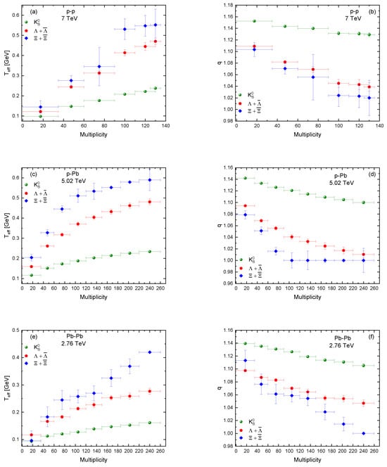
Figure 4. The figures show the effective temperature ($T_{eff}$) and the non-extensive parameter (q) dependence on the event multiplicity for various types of strange particles in different collision scenarios: (i) In proton–proton ($p-p$) collisions at a center-of-mass energy of $\sqrt{s}$ = 7 TeV, given as (a,b). (ii) In proton–lead ($p-Pb$) collisions at a center-of-mass energy of $\sqrt{s}$ = 5.02 TeV, given as (c,d). (iii) In lead–lead ($Pb-Pb$) collisions at a center-of-mass energy of $\sqrt{s}$ = 2.76 TeV, given as (e,f).

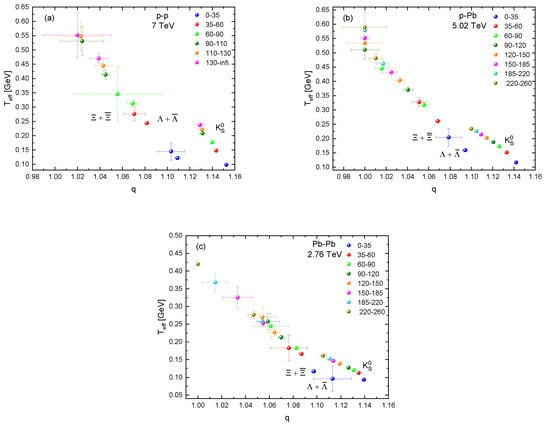
Figure 5. Effective temperature ($T_{eff}$) as a function of non-extensive parameter (q) for different strange particles in different multiplicity slices in (a) $p-p$ collision at $\sqrt{s}$ = 7 TeV, (b) $p-Pb$ collision at $\sqrt{s}$ = 5.02 TeV and (c) $Pb-Pb$ collision at $\sqrt{s}$ = 7 TeV.

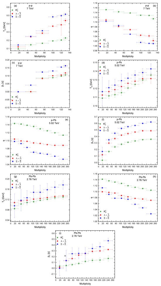
Figure 6. Kinetic freeze-out temperature ($T_0$), non-extensive parameter (q) and transverse flow velocity ${\beta }_T$ as a function of multiplicity for different strange particles in $p-p$, $p-Pb$ and $Pb-Pb$ collisions at $\sqrt{s}$ = 7 TeV, $\sqrt{s_{NN}}$ = 5.02 TeV and $\sqrt{s_{NN}}$ = 2.76 TeV, respectively.

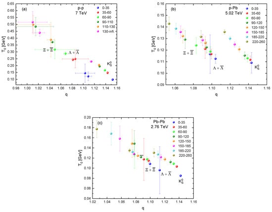
Figure 7. $T_0$ as a function of q for (a) $p-p$ collision at $\sqrt{s}$ = 7 TeV, (b) $p-Pb$ collision at $\sqrt{s_{NN}}$ = 5.02 TeV and (c) $Pb-Pb$ collision at $\sqrt{s_{NN}}$ = 2.76 TeV.

One more interesting observation in the context of symmetric proton–proton ($pp$), lead–lead ($PbPb$), and asymmetric proton–lead ($pPb$) collisions pertains to the distinct behavior of parameter values for heavier baryons. Specifically, these values exhibit a more pronounced rise/fall compared to the corresponding parameter associated with the lighter $K_S^0$ meson in the $pp$ and $PbPb$ scenarios. But in the case of asymmetric $pPb$ collisions, the parameter values for both heavier baryons and the lighter $K_S^0$ meson follow a linear progression, maintaining equal intervals between them.

Figure 5 shows the variation in $T_{eff}$ obtained by the Tsallis distribution function, and Figure 7 shows the variation in $T_0$ obtained by the Equation (2) of the Tsallis function in relation to their respective q parameter. Within these figures, distinct geometrical symbols and colors are utilized to represent different multiplicity segments, indicated as legends in the upper right corner of each plot. The trend showcased in these plots reveals that an increase in the q parameter corresponds to a decrease in both $T_{eff}$ and $T_0$. This observation further leads to the inference that heavier particles exhibit smaller q values, accompanied by larger $T_{eff}$ and $T_0$ values. This pattern lends support to the notion of attaining fast equilibrium and thermal state among the more massive particles. The symmetry and asymmetry observation highlighted earlier is underscored by a distinct and more pronounced distinction observed in the correlation between $T_0$ and q in asymmetric proton–lead ($pPb$) collisions compared to symmetric proton–proton ($pp$) and lead–lead ($PbPb$) collisions.

To provide a comprehensive comparison with existing literature, it is important to note that the study conducted by Murad Badshah and colleagues [13] extensively utilized data from RHIC [37,38,39,40], ALICE [41,42,43], and CMS [44]. Their primary objective was to investigate the centrality dependence of $p_T$ spectra for identified charged hadrons at both 200 GeV and 2.76 TeV. Their results demonstrated a clear trend where both temperature (T) and the average transverse flow velocity ($<{\beta }_T>$) increased as centrality increased. These findings are notably consistent with the observations reported by Olimov et al. [33,34,45]. In our own research, we have observed a similar pattern, with these parameters showing an increase in response to growing particle multiplicity.

In the literature, there are three distinct scenarios: (i) Single Freeze-Out Scenario: in this scenario, particles decouple from the system at the same time or temperature [46]. (ii) Triple Freeze-Out Scenario: this scenario involves three distinct decoupling times or temperatures for identified particles, single strange particles, and multi-strange particles [47]. (iii) Multi-Freeze-Out Scenario: In this scenario, each particle decouples from the system at different times or temperatures. Extensive references to this scenario can be found in the literature [13,48], among others. In the case of simultaneous fitting (in single or even triple freeze-out scenarios), the combined properties such as temperature, flow velocity, and non-extensivity parameters are determined for groups of different particle species. However, this approach does not provide insight into the properties of each individual particle within the group. This can be misleading and lead to a loss of information for each individual particle. Conversely, in the separate fit (multi-freeze-out scenario), the focus is on the properties and interaction mechanisms of each individual particle. This approach minimizes the chances of losing valuable information for each particle.

4. Conclusions

The measurements presented in this study focus on the analyses of the transverse momentum spectra of strange hadrons by Tsallis statistics. The strange particles used are $K_S^0$, $\mathrm{\Lambda }$, and $\mathrm{\Xi }$, in $pp$, $pPb$, and $PbPb$ collisions. The data selected for the analyses were collected and analyzed using the CMS detector at the CERN LHC. We analyzed a wide range of rapidity and event charged-particle multiplicity to examine how the freeze-out parameters, extracted from the $p_T$ spectra of the strange particles, vary with multiplicity and particle species. The $T_{eff}$ and $T_0$ (q) are reported to be increasing (decreasing) with the increase in event charge particle multiplicity, showing a greater temperature and smaller q for particles at higher multiplicity. Similarly, $T_{eff}$ and $T_0$ are found to be decreasing as particle masses drop which shows that lighter particles decouple from the fireball later than heavier particles. Moreover, the non-extensivity parameter is reported to be decreasing with increasing particle masses, confirming the fast equilibrium of the heavier particles than the lighter ones. We found that the average transverse flow velocity increases with multiplicity which indicates the rapid expansion of the fireball at higher multiplicities because of the violent squeeze in the system at such higher multiplicities. Moreover, this increase is observed to be more pronounced for heavier strange particle species in all collision systems ($pp$, $pPb$, and $PbPb$). Furthermore, the study compares the freeze-out parameters differences between different particle species. These differences are more significant in $pp$ and $pPb$ collisions compared to $PbPb$ collisions at similar multiplicities. Furthermore, in symmetric $pp$ and $PbPb$ collisions, parameter values ($q,T_0,{\beta }_T$) exhibit more significant shifts for heavier particles, contrasting the lighter ones. In contrast, in asymmetric $pPb$ collisions, both heavier and lighter particles follow a consistent linear pattern.

References

- Andersen, E.; Antinori, F.; Armenise, N.; Bakke, H.; Bán, J.; Barberis, D.; Beker, H.; Beusch, W.; Bloodworth, I.; Böhm, J.; et al. Enhancement of central Λ, Ξ and Ω yields in Pb-Pb collisions at 158 A GeV/c. Phys. Lett. B 1998, 433, 209–216. [Google Scholar] [CrossRef]
- Adams, J.; Aggarwal, M.; Ahammed, Z.; Amonett, J.; Anderson, B.; Arkhipkin, D.; Averichev, G.; Badyal, S.; Bai, Y.; Balewski, J.; et al. Experimental and theoretical challenges in the search for the quark–gluon plasma: The STAR Collaboration’s critical assessment of the evidence from RHIC collisions. Nucl. Phys. A 2005, 757, 102–183. [Google Scholar] [CrossRef]
- Rafelski, J.; Muller, B. Strangeness production in the quark–gluon plasma. Phys. Rev. Lett. 1982, 48, 1066. [Google Scholar] [CrossRef]
- Abelev, B.I.; Aggarwal, M.M.; Ahammed, Z.; Anderson, B.D.; Arkhipkin, D.; Averichev, G.S.; Bai, Y.; Balewski, J.; Barannikova, O.; Barnby, L.S.; et al. Enhanced strange baryon production in Au+ Au collisions compared to p + p at s NN = 200 GeV. Phys. Rev. C 2008, 77, 044908. [Google Scholar] [CrossRef]
- Andersen, E.; Antinori, F.; Armenise, N.; Bakke, H.; Ban, J.; Barberis, D.; Beker, H.; Beusch, W.; Bloodworth, I.; Bohm, J.; et al. Strangeness enhancement at mid-rapidity in Pb–Pb collisions at 158 A GeV/c. Phys. Lett. B 1999, 449, 401. [Google Scholar] [CrossRef]
- Adams, J.; Adler, C.; Aggarwal, M.M.; Ahammed, Z.; Amonett, J.; Anderson, B.D.; Arkhipkin, D.; Averichev, G.S.; Bai, Y.; Balewski, J.; et al. Multistrange Baryon Production in Au-Au Collisions atsNN = 130 GeV. Phys. Rev. Lett. 2004, 92, 182301. [Google Scholar] [CrossRef]
- Bravina, L.V.; Bugaev, K.A.; Vitiuk, O.; Zabrodin, E.E. Transport Model Approach to Λ and Polarization in Heavy-Ion Collisions. Symmetry 2021, 13, 1852. [Google Scholar] [CrossRef]
- Adcox, K.; Adler, S.; Afanasiev, S.; Aidala, C.; Ajitanand, N.; Akiba, Y.; Al-Jamel, A.; Alexander, J.; Amirikas, R.; Aoki, K.; et al. Formation of dense partonic matter in relativistic nucleus–nucleus collisions at RHIC: Experimental evaluation by the PHENIX Collaboration. Nucl. Phys. A 2005, 757, 184. [Google Scholar] [CrossRef]
- Khachatryan, V.; Sirunyan, A.; Tumasyan, A.; Adam, W.; Asilar, E.; Bergauer, T.; Brandstetter, J.; Brondolin, E.; Dragicevic, M.; Ero, J.; et al. Multiplicity and rapidity dependence of strange hadron production in pp, pPb, and PbPb collisions at the LHC. Phys. Lett. B 2017, 768, 103–129. [Google Scholar] [CrossRef]
- Tsallis, C. Possible generalization of Boltzmann-Gibbs statistics. J. Stat. Phys. 1988, 52, 479. [Google Scholar] [CrossRef]
- Tsallis, C. Nonadditive entropy: The concept and its use. Eur. Phys. J. A 2009, 40, 257. [Google Scholar] [CrossRef]
- Cleymans, J.; Worku, D. The Tsallis distribution in proton-proton collisions at (snn) 1/2 = 0.9 TeV at the LHC. J. Phys. G 2012, 39, 025006. [Google Scholar] [CrossRef]
- Badshah, M.; Ismail, A.H.; Waqas, M.; Ajaz, M.; Mian, M.U.; Dawi, E.A.; Khan, M.A.; AbdelKader, A. Excitation Function of Freeze-Out Parameters in Symmetric Nucleus–Nucleus and Proton–Proton Collisions at the Same Collision Energy. Symmetry 2023, 15, 1554. [Google Scholar] [CrossRef]
- Cleymans, J.; Lykasov, G.I.; Parvan, A.S.; Sorin, A.S.; Teryaev, O.V.; Worku, D. Systematic properties of the Tsallis Distribution: Energy Dependence of Parameters in High-Energy p-p Collisions. Phys. Lett. B 2013, 723, 351. [Google Scholar] [CrossRef]
- Wilk, G.; Wlodarczyk, Z. Interpretation of the Nonextensivity Parameter q in Some Applications of Tsallis Statistics and Lévy Distributions. Phys. Rev. Lett. 2000, 84, 2770. [Google Scholar] [CrossRef]
- Tsallis, C. Enthusiasm and Skepticism: Two Pillars of Science—A Nonextensive Statistics Case. Physics 2022, 4, 609–632. [Google Scholar] [CrossRef]
- PHENIX Collab. Measurement of neutral mesons in p+p collisions at (snn) 1/2 = 200 GeV and scaling properties of hadron production. Phys. Rev. D 2011, 83, 052004. [Google Scholar] [CrossRef]
- Waqas, M.; Peng, G.X.; Ajaz, M.; Ismail, A.H.; Dawi, E.A. Analyses of the collective properties of hadronic matter in Au-Au collisions at 54.4 GeV. Phys. Rev. D 2022, 106, 075009. [Google Scholar] [CrossRef]
- Olimov, K.K.; Iqbal, A. Systematic analysis of midrapidity transverse momentum spectra of identified charged particles in p+p collisions at (snn) 1/2 = 2.76, 5.02, and 7 TeV at the LHC. Int. J. Mod. Phys. A 2020, 35, 2050167. [Google Scholar] [CrossRef]
- Badshah, M.; Waqas, M.; Khubrani, A.M.; Ajaz, M. Systematic analysis of the pp collisions at LHC energies with Tsallis function. Europhys. Lett. 2023, 141, 64002. [Google Scholar] [CrossRef]
- Lao, H.-L.; Liu, F.-H.; Lacey, R.A. Extracting kinetic freeze-out temperature and radial flow velocity from an improved Tsallis distribution. Eur. Phys. J. A 2017, 53, 44. [Google Scholar] [CrossRef]
- Thakur, D.; Tripathy, S.; Garg, P.; Sahoo, R.; Cleymans, J. Indication of a Differential Freeze-Out in Proton-Proton and Heavy-Ion Collisions at RHIC and LHC Energies. Adv. High Energy Phys. 2016, 2016, 4149352. [Google Scholar] [CrossRef]
- Bhattacharyya, T.; Cleymans, J.; Khuntia, A.; Pareek, P.; Sahoo, R. Radial flow in non-extensive thermodynamics and study of particle spectra at LHC in the limit of small (q-1). Eur. Phys. J. A 2016, 52, 30. [Google Scholar] [CrossRef]
- Olimov, K.K.; Kanokova, S.Z.; Olimov, K.; Gulamov, K.G.; Yuldashev, B.S.; Lutpullaev, S.L.; Umarov, F.Y. Average transverse expansion velocities and global freeze-out temperatures in central Cu+Cu, Au+Au, and Pb+Pb collisions at high energies at RHIC and LHC. Mod. Phys. Lett. A 2020, 35, 2050115. [Google Scholar] [CrossRef]
- Khandai, P.K.; Sett, P.; Shukla, P.; Singh, V. System size dependence of hadron pT spectra in p+p and Au+Au collisions at (snn)1/2 = 200 GeV. J. Phys. G 2014, 41, 025105. [Google Scholar] [CrossRef]
- Waqas, M.; Peng, G.X.; Liu, F.-H.; Ajaz, M.; Ismail, A.A.K.H.; Olimov, K.K.; Tawfik, A.N. Particle species and energy dependencies of freeze-out parameters in high-energy proton–proton collisions. Eur. Phys. J. Plus 2022, 137, 1041. [Google Scholar] [CrossRef]
- Tang, Z.; Xu, Y.; Ruan, L.; van Buren, G.; Wang, F.; Xu, Z. Spectra and radial flow in relativistic heavy ion collisions with Tsallis statistics in a blast-wave description. Phys. Rev. C 2009, 79, 051901. [Google Scholar] [CrossRef]
- Wang, S.; Dai, W.; Wang, E.; Wang, X.-N.; Zhang, B.-W. Heavy-Flavour Jets in High-Energy Nuclear Collisions. Symmetry 2023, 15, 727. [Google Scholar] [CrossRef]
- Ajaz, M.; Haj Ismail, A.A.K.; Alrebdi, H.I.; Abdel-Aty, A.-H.; Mian, M.U.; Khan, M.A.; Waqas, M.; Khubrani, A.M.; Wei, H.-R.; AbdelKader, A. Simulation Studies of Track-Based Analysis of Charged Particles in Symmetric Hadron–Hadron Collisions at 7 TeV. Symmetry 2023, 15, 618. [Google Scholar] [CrossRef]
- Khachatryan, V.; The CMS Collaboration; Sirunyan, A.M.; Tumasyan, A.; Adam, W.; Bergauer, T.; Dragicevic, M.; Ero, J.; Fabjan, C.; Friedl, M.; et al. Observation of long-range, near-side angular correlations in proton-proton collisions at the LHC. J. High Energy Phys. 2010, 2010, 91. [Google Scholar] [CrossRef]
- Chatrchyan, S.; Khachatryan, V.; Sirunyan, A.; Tumasyan, A.; Adam, W.; Bergauer, T.; Dragicevic, M.; Ero, J.; Fabjan, C.; Friedl, M.; et al. Multiplicity and transverse momentum dependence of two- and four-particle correlations in pPb and PbPb collisions. Phys. Lett. B 2013, 724, 213–240. [Google Scholar] [CrossRef]
- CMS Collaboration. Measurement of Tracking Efficiency. CMS Physics Analysis Summary CMS-PAS-TRK-10-002 (2010). Available online: http://cdsweb.cern.ch/record/1279139 (accessed on 10 August 2023).
- Olimov, K.K.; Liu, F.H.; Musaev, K.A.; Olimov, K.; Shodmonov, M.Z.; Fedosimova, A.I.; Lebedev, I.A.; Kanokova, S.Z.; Tukhtaev, B.J.; Yuldashev, B.S. Study of midrapidity pt distributions of identified charged particles in Xe+Xe collisions at (snn)1/2 = 5.44 TeV using non-extensive Tsallis statistics with transverse flow. Mod. Phys. Lett. A 2022, 37, 2250095. [Google Scholar] [CrossRef]
- Olimov, K.K.; Liu, F.-H.; Fedosimova, A.I.; Lebedev, I.A.; Deppman, A.; Musaev, K.A.; Shodmonov, M.Z.; Tukhtaev, B.J. Analysis of Midrapidity pT Distributions of Identified Charged Particles in Pb + Pb Collisions at = 5.02 TeV Using Tsallis Distribution with Embedded Transverse Flow. Universe 2022, 8, 401. [Google Scholar] [CrossRef]
- ALICE Collaboration. Production of pions, kaons, (anti-)protons and ϕ mesons in Xe–Xe collisions at = = 5.44 TeV. Eur. Phys. J. C 2021, 81, 584. [Google Scholar] [CrossRef]
- ALICE Collaboration. Production of charged pions, kaons and (anti-)protons in Pb-Pb and inelastic pp collisions at = 5.02 TeV. Phys. Rev. C 2020, 101, 044907. [Google Scholar] [CrossRef]
- Adler, S.S.; Afanasiev, S.; Aidala, C.; Ajitanand, N.N.; Akiba, Y.; Alexander, J.; Amirikas, R.; Aphecetche, L.; Aronson, S.H.; Averbeck, R.; et al. Identified charged particle spectra and yields in Au + Au collisions at sNN =200 GeV. Phys. Rev. C 2004, 69, 034909. [Google Scholar] [CrossRef]
- Adams, J.; Aggarwal, M.M.; Ahammed, Z.; Amonett, J.; Anderson, B.D.; Anderson, M.; Arkhipkin, D.; Averichev, G.S.; Bai, Y.; Balewski, J.; et al. Scaling properties of hyperon production in Au + Au collisions at sNN = 200 GeV. Phys. Rev. Lett. 2007, 98, 062301. [Google Scholar] [CrossRef]
- STAR Collaboration. Identified hadron spectra at large transverse momentum in p+p and d+Au collisions at sNN = 200 GeV. Phys. Lett. B 2006, 637, 161–169. [Google Scholar] [CrossRef]
- Abelev, B. Strange particle production in p + p collisions at = 200 GeV. Phys. Rev. C 2007, 75, 064901. [Google Scholar] [CrossRef]
- Abelev, B. Centrality dependence of π, K, and p production in Pb-Pb collisions at = 2.76 TeV. Phys. Rev. C 2013, 88, 044910. [Google Scholar] [CrossRef]
- Abelev, B. and production in Pb-Pb collisions at sNN = 2.76 TeV. Phys. Rev. Lett. 2013, 111, 222301. [Google Scholar] [CrossRef] [PubMed]
- Abelev, B. Multi-strange baryon production at mid-rapidity in Pb–Pb collisions at sNN = 2.76 TeV. Phys. Lett. B 2014, 728, 216–227. [Google Scholar] [CrossRef]
- The CMSCollaboration; Chatrchyan, S.; Khachatryan, V.; Sirunyan, A.M.; Tumasyan, A.; Adam, W.; Aguilo, E.; Bergauer, T.; Dragicevic, M.; Ero, J.; et al. Study of the inclusive production of charged pions, kaons, and protons in pp collisions at s = 0.9, 2.76, and 7 TeV. Eur. Phys. J. C 2012, 72, 2164. [Google Scholar] [CrossRef]
- Olimov, K.K.; Liu, F.H.; Musaev, K.A.; Olimov, K.; Tukhtaev, B.J.; Yuldashev, B.S.; Saidkhanov, N.S.; Umarov, K.I.; Gulamov, K.G. Gulamov Multiplicity dependencies of midrapidity transverse momentum spectra of identified charged particles in p + p collisions at (s)1/2 = 13 TeV at LHC. Int. J. Mod. Phys. A 2021, 36, 2150149. [Google Scholar] [CrossRef]
- Chatterjee, S.; Mohanty, B.; Singh, R. Freezeout hypersurface at energies available at the CERN Large Hadron Collider from particle spectra: Flavor and centrality dependence. Phys. Rev. C 2015, 92, 024917. [Google Scholar] [CrossRef]
- Waqas, M.; Peng, G.X.; Ajaz, M.; Wazir, Z. Decoupling of non-strange, strange and multi-strange particles from the system in Cu–Cu, Au–Au and Pb–Pb collisions at high energies. Chin. J. Phys. 2022, 77, 1713–1722. [Google Scholar] [CrossRef]
- Chatterjee, S.; Mohanty, B. Production of light nuclei in heavy-ion collisions within a multiple-freezeout scenario. Phys. Rev. C 2014, 90, 034908. [Google Scholar] [CrossRef]
Disclaimer/Publisher’s Note: The statements, opinions and data contained in all publications are solely those of the individual author(s) and contributor(s) and not of MDPI and/or the editor(s). MDPI and/or the editor(s) disclaim responsibility for any injury to people or property resulting from any ideas, methods, instructions or products referred to in the content. |
© 2023 by the authors. Licensee MDPI, Basel, Switzerland. This article is an open access article distributed under the terms and conditions of the Creative Commons Attribution (CC BY) license (https://creativecommons.org/licenses/by/4.0/).