Eigenproblem Basics and Algorithms

Abstract

Some might say that the eigenproblem is one of the examples people discovered by looking at the sky and wondering. Even though it was formulated to explain the movement of the planets, today it has become the ansatz of solving many linear and nonlinear problems. Formulation in the terms of the eigenproblem is one of the key tools to solve complex problems, especially in the area of molecular geometry. However, the basic concept is difficult without proper preparation. A review paper covering basic concepts and algorithms is very useful. This review covers the basics of the topic. Definitions are provided for defective, Hermitian, Hessenberg, modal, singular, spectral, symmetric, skew-symmetric, skew-Hermitian, triangular, and Wishart matrices. Then, concepts of characteristic polynomial, eigendecomposition, eigenpair, eigenproblem, eigenspace, eigenvalue, and eigenvector are subsequently introduced. Faddeev–LeVerrier, von Mises, Gauss–Jordan, Pohlhausen, Lanczos–Arnoldi, Rayleigh–Ritz, Jacobi–Davidson, and Gauss–Seidel fundamental algorithms are given, while others (Francis–Kublanovskaya, Gram–Schmidt, Householder, Givens, Broyden–Fletcher–Goldfarb–Shanno, Davidon–Fletcher–Powell, and Saad–Schultz) are merely discussed. The eigenproblem has thus found its use in many topics. The applications discussed include solving Bessel’s, Helmholtz’s, Laplace’s, Legendre’s, Poisson’s, and Schrödinger’s equations. The algorithm extracting the first principal component is also provided.

1. Introduction

About 250 years ago, the study of the motion of rigid bodies, with direct interest to the movement of the planets, led to the first formulation of the eigenproblem. In general, the eigenproblem is about minimization of the maximum eigenvalue of an matrix that depends affinely on a variable, subject to some constraint. Euler [1], Lagrange [2], Laplace [3], Fourier [4], and Cauchy [5] studied the problem.

Linear algebra was introduced through systems of linear equations. The terms matrix, determinant, and minor, as are used today, were introduced by Sylvester around the year 1850 [6].

Symmetry plays an essential role. Symmetric real-valued matrices have real eigenvalues. Hermite [7] extended this result to complex valued matrices mirroring the conjugate transpose (Hermitian matrices), and Sylvester [8] to Hessians (Hessian matrices).

Some authors [9] noted “any attempt to write a complete overview on the research on computational aspects of the eigenvalue problem a hopeless task”. Here, no such thing is claimed, and instead for the eigenproblem is provided a bottom-up approach, from simple to complex on the one hand and from old to new on the other hand. The style used in specifying the algorithms was previously used in [10].

As mentioned before, the characteristic polynomial and the eigenproblem appeared for the first time in the context of solving complex problems in physics, but the area of their use has been expanded since, and today covers a diverse set of applications. Even if, in most instances, the problems involve operating on real-valued data ($\mathbb{R}$), in some cases, the mathematical and numerical treatise has proved to be more convenient in the complex domain ($\mathbb{C}$), and the literature on calling for eigenproblem and characteristic polynomial formulations and solutions is expanding and growing. Since a real number can always be seen as a particular case of a complex number, a number can be seen as a particular case of an 1-tuple (or a vector with one component), or a matrix with only one entry. Thus, since the eigenproblem is formulated and uses all these fields (a field is generally a set of elements having defined multiplication and addition operations analogous to multiplication and addition in the real number system), the tendency to generalize is perfectly justified, so $\mathbb{K}$ will be referred to the field generalizing those alternatives.

Generally, a matrix is an ordered set of values. Formally, a matrix is a two-dimensional arrangement of its values. Sylvester [6] appears to be the first to use the arrangement of the matrix elements in rows and columns. A square matrix has an equal number of columns and rows. Thus, if $A=\left(a_{i,j}\right)\in {\mathbb{K}}^{n\times n}$ (in general $m\ne n$) is a square matrix, then $a_{i,j}\in \mathbb{K}$ are the elements of the matrix for each $i=1,\dots ,n$ and $j=1,\dots ,n$ (integers). On the field ($\mathbb{K})$, one can recognize the existence of the addition ($C=A+B$, defined as $c_{i,j}=a_{i,j}+b_{i,j}$ for all $1\le i,j\le n$), and that of the multiplication ($C=A\times B$, defined as $c_{i,j}={\sum }_{k=1}^n{a}_{i,k}\times b_{k,j}$ for all $1\le i,j\le n$). A second multiplication operation ($C=\alpha \times A$, defined as $c_{i,j}=\alpha \times a_{i,j}$ for any $\alpha \in \mathbb{K}$ and all $1\le i,j\le n$) provides a linear space. One immediate consequence is the existence of the subtraction ($C=A-B$, defined as $c_{i,j}=a_{i,j}-b_{i,j}$ for all $1\le i,j\le n$).

Two particular matrices are of importance: the zero valued ($O=\left({\omega }_{i,j}\right)\in {\mathbb{K}}^{n\times n},{\omega }_{i,j}=0$ for all $1\le i,j\le n$), and the identity matrix ($I=\left({\iota }_{i,j}\right)\in {\mathbb{K}}^{n\times n},{\iota }_{i,j}={\delta }_{i,j}$ for all $1\le i,j\le n$ and ${\delta }_{i,j}$ is the Kronecker delta [11]).

Two matrix operations are also of importance: the transpose ($C=A^T,$ defined as $c_{i,j}=a_{j,i}$ for all $1\le i,j\le n$), and the conjugate ($C=\overline{A},$ defined as $c_{i,j}=\overline{a_{i,j}}$ for all $1\le i,j\le n$).

2. Basic Concepts

Definition 1.

Characteristic polynomial.

The characteristic polynomial P (in $\lambda$) associated with $A\in {\mathbb{K}}^{n\times n}$ is:

$$P(\lambda ,A)\leftarrow |\lambda \times I-A|$$

(1)

where $|·|$ (symbolically) evaluates the determinant. The characteristic polynomial is always a monic polynomial (leading coefficient is 1) of degree n.

Definition 2.

Eigenvalue.

An eigenvalue (of A) is a root of the characteristic equation:

$$\lambda \mathrm{eigenvalue}\mathrm{of}A\stackrel{\hspace{1em} }{\iff }|\lambda \times I-A|=0$$

(2)

Equation (2) always has n roots, even if some of them may not be distinct, but multiple. Equation (2) provides all eigenvalues of A.

Definition 3.

Eigenproblem.

The eigenproblem is:

$$\mathrm{For}A\in {\mathbb{K}}^{n\times n}\mathrm{determine}\lambda \in \mathbb{K}\mathrm{and}v\in {\mathbb{K}}^n,v\ne 0,\mathrm{s}.\mathrm{t}.A\times v=\lambda \times v$$

(3)

In Equation (3), $\lambda$ is an eigenvalue and v is an eigenvector of A, while the $(\lambda ,v)$ pair is an eigenpair of A. One should notice that Equation (2) provides a direct method for calculation of the eigenvalues, which, when inserted in Equation (3), provides their associated eigenvectors. The set $\{v:(\lambda \times I-A)v=0\}$ is the eigenspace of A associated with $\lambda$ being the union of the zero vector with the set of all eigenvectors of A associated with $\lambda$ (nullspace of $\lambda \times I-A$). Furthermore, any nonzero scalar multiple of an eigenvector is also an eigenvector, so unit eigenvectors may be provided when convenient.

The eigenproblem is generalized when another matrix, B ($B\in {\mathbb{K}}^{n\times n}$), is inserted in Equation (3): $A\times v$ = $\lambda \times B\times v$.

Example 1.

$\mathbb{K}=\mathbb{C}$.

Let us consider two complex valued matrices with a certain similarity in their structure (Table 1, $i\leftarrow \sqrt{-1}$).

Table 1. Eigenproblem of two complex matrices containing the roots of $y^4=1$.

A	1	2	3	4
1	1	i	$-1$	$-i$
2	i	$-1$	$-i$	1
3	$-1$	$-i$	1	i
4	$-i$	1	i	$-1$
$P(\lambda ,A)={\lambda }^4$; eigenvector of $\lambda =-2$: ${\left[\begin{array}{cccc}i& -1& -i& 1\end{array}\right]}^{\mathrm{T}}$
B	1	2	3	4
1	$-1$	1	i	$-i$
2	$-i$	i	$-1$	1
3	1	$-1$	$-i$	i
4	i	$-i$	1	$-1$
$P(\lambda ,B)=(\lambda +2){\lambda }^3$; eigenvector of $\lambda =0$: ${\left[\begin{array}{cccc}-i& 1& 0& 0\end{array}\right]}^{\mathrm{T}}$; eigenvector of $\lambda =0$: ${\left[\begin{array}{cccc}1& 1& 0& 0\end{array}\right]}^{\mathrm{T}}$

One should notice that matrix A contains the same elements as matrix B, but with an increased symmetry, a property that is transferred to the eigenspace, since the eigenvector of matrix A is the dot product of the eigenvectors of matrix B. More about real eigenvalues of complex valued matrices can be found in [12] regarding their applications in signal processing [13].

Example 2.

Molecular topology.

A chemical compound—namely 1,4,2,5-diazadiborine—compound 8 in [14] was geometrically represented [14,15], and the topological distance matrix was calculated on the heavy atoms skeleton ([Di] in Figure 5 from [15]). Here, the topological distance matrix (Table 2) is used to exemplify the eigenproblem on $\mathbb{K}=\mathbb{R}$.

Table 2. Eigenproblem of a symmetrical matrix from ${\mathbb{R}}^{6\times 6}$.

A	1	2	3	4	5	6
1	0	1	2	3	2	1
2	1	0	1	2	3	2
3	2	1	0	1	2	3
4	3	2	1	0	1	2
5	2	3	2	1	0	1
6	1	2	3	2	1	0
Eigenvalue	Eigenvector
−4	${\left[\begin{array}{cccccc}-1& -1& 0& 1& 1& 0\end{array}\right]}^{\mathrm{T}}$
−1	${\left[\begin{array}{cccccc}-1& 1& -1& 1& -1& 1\end{array}\right]}^{\mathrm{T}}$
0	${\left[\begin{array}{cccccc}-1& 1& 0& -1& 1& 0\end{array}\right]}^{\mathrm{T}}$
9	${\left[\begin{array}{cccccc}1& 1& 1& 1& 1& 1\end{array}\right]}^{\mathrm{T}}$

The characteristic polynomial of the matrix A from Table 2 is: $P(\lambda ,A)={(\lambda +4)}^2(\lambda +1){\lambda }^2(\lambda -9)$. One should notice that there are only four distinct eigenvalues here (−4, −1, 0, and 9), so there are only four distinct unit eigenvectors as well. A (square) matrix is diagonal if the entries outside the main diagonal are all zero (with z as an arbitrary value):

$$A\in {\mathbb{K}}^{n\times n}\mathrm{diagonal}\stackrel{\hspace{1em} }{\iff }{a}_{i,j}=\left\{\begin{array}{cc}0\hfill & \mathrm{if}i\ne j\hfill \\ z\in \mathbb{K}\hfill & \mathrm{otherwise}\hfill \end{array}\right.$$

(4)

A square matrix is invertible if its inverse exists ($B=A^{-1}$ in Equation (5)):

$$A\in {\mathbb{K}}^{n\times n}\mathrm{invertible}\stackrel{\hspace{1em} }{\iff }\exists B\in {\mathbb{K}}^{n\times n}\mathrm{s}.\mathrm{t}.A\times B=I=B\times A$$

(5)

A square matrix is diagonalizable if a diagonal form is obtainable:

$$A\in {\mathbb{K}}^{n\times n}\mathrm{diagonalizable}\stackrel{\hspace{1em} }{\iff }\exists B\in {\mathbb{K}}^{n\times n}\mathrm{invertible}\mathrm{s}.\mathrm{t}.B^{-1}\times A\times B\mathrm{diagonal}$$

(6)

If $D\leftarrow B^{-1}\times A\times B$ from Equation (6), then $B\times D\times B^{-1}$ is the eigendecomposition of A ($A=B\times D\times B^{-1}$).

If $A\in {\mathbb{K}}^{n\times n}$ has n distinct eigenvalues (${\lambda }_i$, $i=1,\dots ,n$), then it has n linearly independent eigenvectors ($v_i$, $i=1,\dots ,n$). M, constructed from its eigenvectors as columns (${M^T}_i\leftarrow v_i$), is the modal matrix(of A), and $M^{-1}\times A\times M$ is the spectral matrix(of A) and is a diagonal matrix with the eigenvalues of A on the main diagonal [16] (and $M^{-1}=M^H$).

On the contrary, a defective matrix is a square matrix that does not have a complete basis of eigenvectors, and is therefore not diagonalizable.

3. Algorithms

Algorithm 1 shows the characteristic polynomial coefficients and roots.

Given a matrix, A, the coefficients of the characteristic polynomial (Equation (1)) can be easily provided by an algorithm that was first suggested by LeVerrier [17]. One good alternative to provide the roots of the characteristic polynomial when all its coefficients are real is [18]. Other recently reported alternatives for finding roots include [19,20].

Algorithm 1 Faddeev–LeVerrier

Input: A     //square matrix  function Faddeev($\&A$)     // Trace, UnitM, MultC, AddM, MultM defined in Appendix A     $n\leftarrow \text{COUNT}\left(A\right)$; $B\leftarrow A$; $c\leftarrow \left[\right]$; $c\left[0\right]\leftarrow 1$     For($i\leftarrow 1$; $i\le n$; $i\leftarrow i+1$)        $c\left[k\right]\leftarrow -\mathrm{T}\text{RACE}\left(B\right)/i$; $D\leftarrow \mathrm{U}\text{NIT}\mathrm{M}\left(n\right)$; $D\leftarrow \mathrm{M}\text{ULT}\mathrm{C}\left(c\right[k],D)$        $B\leftarrow \mathrm{A}\text{DD}\mathrm{M}(B,D)$; $B\leftarrow \mathrm{M}\text{ULT}\mathrm{M}(A,B)$     EndFor     $\text{RETURN}\left(c\right)$    // $c\leftarrow ChP\left(A\right)$  end function  $c\leftarrow \mathrm{F}\text{ADDEEV}\left(A\right)$    // c is the characteristic polynomial of A Output: c    // c is the characteristic polynomial of A

Algorithm 2 shows the von Mises iteration.

Given a diagonalizable matrix, A, the von Mises iteration [21] will produce a nonzero vector, v, and a corresponding eigenvector of ${\lambda }_1$ and A, that is, $Av={\lambda }_{1}v$, where ${\lambda }_1$ is the greatest (in absolute value) eigenvalue of A.

The von Mises iteration starts with an approximation to the dominant eigenvector or a random vector, $v_0$, and uses the recurrence relation (7) ($k=0,1,\dots$).

$$v_{k+1}\leftarrow \frac{A\times v_k}{\parallel A\times v_k\parallel }$$

(7)

Let us consider the Example 2 eigenproblem, in which the greatest eigenvalue is 9 and its associated eigenvector is ${\left[\begin{array}{cccccc}1& 1& 1& 1& 1& 1\end{array}\right]}^T$. Table 3 lists a series of case studies regarding the convergence of Algorithm 1.

Table 3. Case studies of Algorithm 2 convergence for the Example 2 eigenproblem.

Case	Initial Eigenvector	Iterations	Note
1	${\left[\begin{array}{cccccc}1& 1& 1& 1& 1& 1\end{array}\right]}^{\mathrm{T}}$	1	Iterations is the number of Equation (7) iterations to acquire an residual error less than $5\times {10}^{-5}$ for each component of the final eigenvector (each is then approximately 1.0000). Final eigenvector: ${\left[\begin{array}{cccccc}1.0000& 1.0000& 1.0000& 1.0000& 1.0000& 1.0000\end{array}\right]}^{\mathrm{T}}$.
2	${\left[\begin{array}{cccccc}0& 1& 1& 1& 1& 1\end{array}\right]}^{\mathrm{T}}$	12
3	${\left[\begin{array}{cccccc}0& 0& 1& 1& 1& 1\end{array}\right]}^{\mathrm{T}}$	13
4	${\left[\begin{array}{cccccc}0& 0& 0& 1& 1& 1\end{array}\right]}^{\mathrm{T}}$	14
5	${\left[\begin{array}{cccccc}0& 0& 0& 0& 1& 1\end{array}\right]}^{\mathrm{T}}$	14
6	${\left[\begin{array}{cccccc}0& 0& 0& 0& 0& 1\end{array}\right]}^{\mathrm{T}}$	14

The algorithm implementing von Mises iteration is given as Algorithm 2.

Algorithm 2 Principal eigenvector

Input: A    //diagonalizable matrix  procedure Principal($\&A,\&v$)     $M\_Eps\leftarrow {10}^{-7}$     For( ; ; )        $w\leftarrow \mathrm{M}\text{ULT}\mathrm{M}(A,v)$; $w\leftarrow \mathrm{U}\text{NIT}\mathrm{V}\left(w\right)$        If($\mathrm{D}\text{IFF}\mathrm{V}(v,w)$ < $M\_Eps$) $\mathrm{B}\text{REAK}$ Else $v\leftarrow w$ EndIf     EndFor     $v\leftarrow w$  end procedure  $n\leftarrow \text{COUNT}\left(A\right)$; $v\leftarrow \mathrm{I}\text{NIT}\mathrm{V}(n,1)$    // $v\leftarrow 1$; $\mathrm{I}\text{NIT}\mathrm{V}(n,-1)$ for $v\leftarrow \text{RAND}$  $\mathrm{P}\text{RINCIPAL}(A,v)$    // v is the principal eigenvector of A Output: v    // v is the principal eigenvector of A

If ${\lambda }_1$ is strictly greater in magnitude than other eigenvalues of A, and the starting vector, $v_0$, has a nonzero component in the direction of an eigenvector associated with ${\lambda }_1$, then $v_k$ converges to an eigenvector associated with ${\lambda }_1$. Without the two assumptions above, $v_k$ does not necessarily converge. The convergence is geometric, with the ratio $|{\lambda }_2/{\lambda }_1|$, where ${\lambda }_2$ denotes the second dominant eigenvalue. The convergence is slow if ${\lambda }_2$ is close in magnitude to ${\lambda }_1$.

Algorithm 3 shows the Gauss–Jordan elimination.

Given a diagonalizable matrix, A, and an eigenvalue, $\lambda$, the Gauss–Jordan elimination [22] is able to provide the diagonalized matrix, a basis to derive a nonzero eigenvector, v. It is given as Algorithm 3.

Consider again the Example 2 eigenproblem, in which the goal now is to obtain the eigenvectors associated with the eigenvalues.

It should be noticed that $C\times v=0$ from Table 4 has one degree of freedom (diagonalization produced a zero on the main diagonal of matrix C in Table 4, $v_6$ in $C\times v$), therefore any arbitrary value ($v_6\ne 0$, since it must be $v\ne 0$) of its associated variables will provide an eigenvalue. For instance, $v_6\leftarrow 1$ will provide the same solution as the one listed in Table 2 ($v_6=v_5=v_4=v_3=v_2=v_1=1$). Additionally, while $C\times v=0$ has one degree of freedom by necessity, $\lambda =9$ has a multiplicity of 1 in $|\lambda \times I-A|=0$ (indeed, see Example 2).

Algorithm 3 Matrix diagonalization

Input: A    //a square diagonalizable matrix  procedure GaussJ($\&A,\&B,\&C$)     $n\leftarrow \text{COUNT}\left(A\right)$; $M\_Eps\leftarrow {10}^{-7}$     For($i\leftarrow 0$; $i<n$; $i\leftarrow i+1$)        $k\leftarrow i$        For($j\leftarrow i+1$; $j<n$; $j\leftarrow j+1$) If($\left|a\right[j\left]\right[i\left]\right|>\left|a\right[k\left]\right[i\left]\right|$) $k\leftarrow j$ EndIf EndFor        If($\left|a\right[i\left]\right[k\left]\right|<M\_Eps$) $\text{CONTINUE}$ EndIf        If($k\ne i$)           $x\leftarrow c\left[k\right]$; $c\left[k\right]\leftarrow c\left[i\right]$; $c\left[i\right]\leftarrow x$           For($j\leftarrow 0$; $j<n$; $j\leftarrow j+1$) $x\leftarrow b\left[k\right]\left[j\right]$; $b\left[k\right]\left[j\right]\leftarrow b\left[i\right]\left[j\right]$; $b\left[i\right]\left[j\right]\leftarrow x$ EndFor           For($j\leftarrow 0$; $j<n$; $j\leftarrow j+1$) $x\leftarrow a\left[k\right]\left[j\right]$; $a\left[k\right]\left[j\right]\leftarrow a\left[i\right]\left[j\right]$; $a\left[i\right]\left[j\right]\leftarrow x$ EndFor        EndIf        $x\leftarrow a\left[i\right]\left[i\right]$; $c\left[i\right]\leftarrow c\left[i\right]/x$        For($j\leftarrow 0$; $j<n$; $j\leftarrow j+1$) $b\left[i\right]\left[j\right]\leftarrow b\left[i\right]\left[j\right]/x$; $a\left[i\right]\left[j\right]\leftarrow a\left[i\right]\left[j\right]/x$ EndFor        For($j\leftarrow 0$; $j<n$; $j\leftarrow j+1$) If($i\ne j$)           $x\leftarrow a\left[j\right]\left[i\right]$; $c\left[j\right]\leftarrow c\left[j\right]-x·c\left[i\right]$           For($k\leftarrow 0$; $i<n$; $k\leftarrow k+1$) $b\left[j\right]\left[k\right]\leftarrow b\left[j\right]\left[k\right]-x·b\left[i\right]\left[k\right]$ EndFor           For($k\leftarrow 0$; $i<n$; $k\leftarrow k+1$) $a\left[j\right]\left[k\right]\leftarrow a\left[j\right]\left[k\right]-x·a\left[i\right]\left[k\right]$ EndFor        EndIf EndFor  end procedure  $\mathrm{G}\text{AUSS}\mathrm{J}(A,B,C)$    // square matrix A is diagonalized here Output: A    // $A\leftarrow \mathrm{diagonalized}A$, $B\leftarrow A^{-1}$ if exists, $C\leftarrow A^{-1}C$ if exists

Table 4. Diagonalization of $9·I-A$ (Table 2, Example 2).

B	1	2	3	4	5	6	C	1	2	3	4	5	6
1	9	−1	−2	−3	−2	−1	1	1	0	0	0	0	−1	$C\times \left[\begin{array}{c}{v}_1\\ v_2\\ v_3\\ v_4\\ v_5\\ v_6\end{array}\right]=\left[\begin{array}{c}{v}_1-v_6\\ v_2-v_6\\ v_3-v_6\\ v_4-v_6\\ v_5-v_6\\ 0\end{array}\right]$
2	−1	9	−1	−2	−3	−2	2	0	1	0	0	0	−1
3	−2	−1	9	−1	−2	−3	3	0	0	1	0	0	−1
4	−3	−2	−1	9	−1	−2	4	0	0	0	1	0	−1
5	−2	−3	−2	−1	9	−1	5	0	0	0	0	1	−1
6	−1	−2	−3	−2	−1	9	6	0	0	0	0	0	0

$B\leftarrow 9·I-A$; C from Algorithm 3 on B.

$C\times v=0$ from Table 5 has two degrees of freedom (diagonalization produced two zeroes on the main diagonal of matrix C in Table 5, $v_5$ and $v_6$ in $C\times v$), so any arbitrary value ($v_5·v_6\ne 0$, since it must be $v\ne 0$) of its associated variable will provide an eigenvalue. For instance, $v_5\leftarrow 1$ and $v_6\leftarrow 0$ will provide the same solution as the one listed in Table 2 ($v_6=v_3=0$, $v_5=v_4=1$, $v_2=v_1=-1$). Furthermore, while $C\times v=0$ has two degrees of freedom by necessity, $\lambda =-4$ has a multiplicity of 2 in $|\lambda \times I-A|=0$ (indeed, see Example 2).

Table 5. Diagonalization of $-4·I-A$ (Table 2, Example 2).

B	1	2	3	4	5	6	C	1	2	3	4	5	6
1	−4	−1	−2	−3	−2	−1	1	1	0	0	0	1	−1	$C\times \left[\begin{array}{c}{v}_1\\ v_2\\ v_3\\ v_4\\ v_5\\ v_6\end{array}\right]=\left[\begin{array}{c}{v}_1+v_5-v_6\\ v_2+v_5\\ v_3+v_6\\ v_4-v_5+v_6\\ 0\\ 0\end{array}\right]$
2	−1	−4	−1	−2	−3	−2	2	0	1	0	0	1	0
3	−2	−1	−4	−1	−2	−3	3	0	0	1	0	0	1
4	−3	−2	−1	−4	−1	−2	4	0	0	0	1	−1	1
5	−2	−3	−2	−1	−4	−1	5	0	0	0	0	0	0
6	−1	−2	−3	−2	−1	−4	6	0	0	0	0	0	0

$B\leftarrow -4·I-A$; C from Algorithm 3 on B.

$C\times v=0$ from Table 6 has one degree of freedom (diagonalization produced one zero on the main diagonal of matrix C in Table 6, $v_6$ in $C\times v$), so any arbitrary value ($v_6\ne 0$, since it must be $v\ne 0$) of its associated variable will provide an eigenvalue. For instance, $v_6\leftarrow zzz$ will provide the same solution as the one listed in Table 2 ($v_6=v_4=v_2=1$, $v_5=v_3=v_1=-1$). Additionally, while $C\times v=0$ has one degree of freedom by necessity, $\lambda =-1$ has a multiplicity of 1 in $|\lambda \times I-A|=0$ (indeed, see Example 2).

Table 6. Diagonalization of $-1·I-A$ (Table 2, Example 2).

B	1	2	3	4	5	6	C	1	2	3	4	5	6
1	−1	−1	−2	−3	−2	−1	1	1	0	0	0	0	1	$C\times \left[\begin{array}{c}{v}_1\\ v_2\\ v_3\\ v_4\\ v_5\\ v_6\end{array}\right]=\left[\begin{array}{c}{v}_1+v_6\\ v_2-v_6\\ v_3+v_6\\ v_4-v_6\\ v_5+v_6\\ 0\end{array}\right]$
2	−1	−1	−1	−2	−3	−2	2	0	1	0	0	0	−1
3	−2	−1	−1	−1	−2	−3	3	0	0	1	0	0	1
4	−3	−2	−1	−1	−1	−2	4	0	0	0	1	0	−1
5	−2	−3	−2	−1	−1	−1	5	0	0	0	0	1	1
6	−1	−2	−3	−2	−1	−1	6	0	0	0	0	0	0

$B\leftarrow -1·I-A$; C from Algorithm 3 on B.

$C\times v=0$ from Table 7 has two degrees of freedom (diagonalization produced two zeroes on the main diagonal of matrix C in Table 7, $v_5$ and $v_6$ in $C\times v$), so any arbitrary value ($v_5·v_6\ne 0$, since it must be $v\ne 0$) of its associated variable will provide an eigenvalue. For instance, $v_5\leftarrow 1$ and $v_6\leftarrow 0$ will provide the same solution as the one listed in Table 2 ($v_6=v_3=0$, $v_5=v_2=1$, $v_4=v_1=-1$). Furthermore, while $C\times v=0$ has two degrees of freedom by necessity, $\lambda =0$ has a multiplicity of 2 in $|\lambda \times I-A|=0$ (indeed, see Example 2).

Table 7. Diagonalization of $0·I-A$ (Table 2, Example 2).

B	1	2	3	4	5	6	C	1	2	3	4	5	6
1	0	−1	−2	−3	−2	−1	1	1	0	0	0	1	1	$C\times \left[\begin{array}{c}{v}_1\\ v_2\\ v_3\\ v_4\\ v_5\\ v_6\end{array}\right]=\left[\begin{array}{c}{v}_1+v_5+v_6\\ v_2-v_5\\ v_3-v_6\\ v_4+v_5+v_6\\ 0\\ 0\end{array}\right]$
2	−1	0	−1	−2	−3	−2	2	0	1	0	0	−1	0
3	−2	−1	0	−1	−2	−3	3	0	0	1	0	0	−1
4	−3	−2	−1	0	−1	−2	4	0	0	0	1	1	1
5	−2	−3	−2	−1	0	−1	5	0	0	0	0	0	0
6	−1	−2	−3	−2	−1	0	6	0	0	0	0	0	0

$B\leftarrow 0·I-A$; C from Algorithm 3 on B.

Algorithm 4 shows inverse iteration.

Inverse iteration appears to have originally been developed by Ernst Pohlhausen [23] with the purpose of computing resonance frequencies in structural mechanics.

If ${\kappa }_i\in \mathbb{K}$ is not an eigenvalue of A, then $(A-{\kappa }_i\times I)$ is invertible. The eigenvectors of ${(A-{\kappa }_i\times I)}^{-1}$ are the same as the eigenvectors of A, and the corresponding eigenvalues are $\left\{{({\lambda }_j-{\kappa }_i)}^{-1}\right\}$, where $\left\{{\lambda }_j\right\}$ are the eigenvalues of A.

If ${\kappa }_i\leftarrow {\lambda }_i-ϵ$, with ${\lambda }_i$ the eigenvalue of A, and $ϵ$ being very small, then ${({\lambda }_i-{\kappa }_i)}^{-1}$ is much larger than ${({\lambda }_j-{\kappa }_i)}^{-1}$ for all $j\ne i$. Thus, Algorithm 2 (principal eigenvector) on ${(A-{\kappa }_{i}I)}^{-1}$ will converge rapidly. This idea is called inverse iteration and is implemented as Algorithm 4.

Algorithm 4 Inverse iteration to eigenspaces

Input: $A,v$    //a square diagonalizable matrix A and its eigenvalues v  procedure InvIt($A,w$)     $n\leftarrow \text{COUNT}\left(A\right)$; $E\_Eps\leftarrow {10}^{-4}$; $w\leftarrow w-E\_Eps$     $v\leftarrow \mathrm{I}\text{NIT}\mathrm{V}(n,-1)$    // $v\leftarrow \text{RAND}$     For($i\leftarrow 0$; $i<n$; $i\leftarrow i+1$) $A\left[i\right]\left[i\right]\leftarrow A\left[i\right]\left[i\right]-w$ EndFor     $\mathrm{G}\text{AUSS}\mathrm{J}(A,B,C)$; $\mathrm{P}\text{RINCIPAL}(B,v)$; $\text{RETURN}\left(v\right)$    // v is an eigenvector of w  end procedure  $m\leftarrow \text{COUNT}\left(v\right)$; For($i\leftarrow 0$; $i<m$; $i\leftarrow i+1$) $u\left[i\right]\leftarrow \mathrm{I}\text{NV}\mathrm{I}\text{T}(A,v[i\left]\right)$ EndFor Output: u    // eigenvectors of A

Taking into consideration the data from Example 2 again, the output of Algorithm 4 is given in Table 8.

Table 8. Algorithm 4 output for Example 2 eigenproblem.

Eigenvalue	Eigenvector	Wrong Eigenvector
−4	${\left[\begin{array}{cccccc}-1& 1& 2& 1& -1& -2\end{array}\right]}^{\mathrm{T}}$	${\left[\begin{array}{cccccc}1& 1& 1& 1& 1& 1\end{array}\right]}^{\mathrm{T}}$
−1	${\left[\begin{array}{cccccc}-1& 1& -1& 1& -1& 1\end{array}\right]}^{\mathrm{T}}$	${\left[\begin{array}{cccccc}1& 1& 1& 1& 1& 1\end{array}\right]}^{\mathrm{T}}$
0	${\left[\begin{array}{cccccc}1& 1& -2& 1& 1& -2\end{array}\right]}^{\mathrm{T}}$	${\left[\begin{array}{cccccc}1& 1& 1& 1& 1& 1\end{array}\right]}^{\mathrm{T}}$
9	${\left[\begin{array}{cccccc}1& 1& 1& 1& 1& 1\end{array}\right]}^{\mathrm{T}}$	${\left[\begin{array}{cccccc}1& 1& 1& 1& 1& 1\end{array}\right]}^{\mathrm{T}}$
	$v\leftarrow \mathrm{RAND}$ in Algorithm 4	$v\leftarrow 1$ in Algorithm 4

One should notice that, for the multiple eigenvalues ($\lambda \in \{-4,0\}$) of A from Table 2, the solution provided from diagonalization ($v_5\leftarrow 1$ and $v_6\leftarrow 0$ in Table 5 and Table 7, respectively, eigenvectors in Table 2) and the solution provided by inverse iteration (Table 8) are different, but belong to the same eigenspace ($v_5\leftarrow -1$ and $v_6\leftarrow -2$ in Table 5 for the eigenvector associated with the $-4$ eigenvalue in Table 8; $v_5\leftarrow 1$ and $v_6\leftarrow -2$ in Table 7 for the eigenvector associated with the 0 eigenvalue in Table 8). Of course, this is due to the presence of the random effect (see $\mathrm{RAND}$ in Algorithm 4).

The $\mathrm{RAND}$ has been used instead of a fixed value initialization, because if (by any chance) the initial eigenvector ($v\leftarrow \mathrm{I}\text{NIT}\mathrm{V}(n,-1)$ in Algorithm 4) is colinear with an eigenvector of another eigenvalue (and ${\left[\begin{array}{cccccc}1& 1& 1& 1& 1& 1\end{array}\right]}^{\mathrm{T}}$ is the eigenvector of the 9 eigenvalue, see Table 8), then the convergence fails (see Table 8).

Formally, given a diagonalizable matrix, A, inverse iteration [21] will iterate an approximate eigenvector ($v_{i,k+1}$) when an approximation, ${\kappa }_i$ (${\kappa }_i\leftarrow {\lambda }_i-ϵ$, $ϵ$ small), to a corresponding eigenvalue (${\lambda }_i$) is used to form ${(A-{\kappa }_i\times I)}^{-1}$ (Equation (8)), being conceptually similar to the power method (Equation (7)). Inverse iteration starts with a random vector, $v_{i,0}$, associated with a ${\lambda }_i$ eigenvalue and uses the recurrence relation 8 ($k=0,1,\dots$).

$$v_{i,k+1}\leftarrow \frac{{(A-{\kappa }_i\times I)}^{-1}\times v_{i,k}}{\parallel {(A-{\kappa }_i\times I)}^{-1}\times v_{i,k}\parallel }$$

(8)

For big systems, the direct calculation of the characteristic polynomial roots (via Algorithm 1, for instance) may be more than a processor with simple or double precision floating point numbers can handle. Of course, one alternative is to increase the precision, but another alternative is to use a method that adjusts the eigenvalue and the eigenvector at the same time. A modification to the inverse method will provide such an alternative. It should be noted that an approximation of the eigenvalue can be obtained from ${\kappa }_{i,k+1}\leftarrow v_{i,k}^T\times A\times v_{i,k}$, and then the initialization is $v_{i,0}\leftarrow \mathrm{RAND}$ and ${\kappa }_{i,0}\leftarrow {\lambda }_i-ϵ$, and relation (8) is changed into system (9) (Rayleigh quotient iteration, or Ritz method [24]).

$$\left\{\begin{array}{c}{v}_{i,k+1}\leftarrow {\displaystyle \frac{{(A-{\kappa }_{i,k}\times I)}^{-1}\times v_{i,k}}{\parallel {(A-{\kappa }_{i,k}\times I)}^{-1}\times v_{i,k}\parallel }}\hfill \\ {\kappa }_{i,k+1}\leftarrow v_{i,k+1}^T\times A\times v_{i,k+1}\hfill \end{array}\right.k=0,1,\dots$$

(9)

Other aspects of inverse iteration are discussed in [25].

Algorithm 5 shows reducing complexity.

The complexity of the eigenproblem is a function of the dimension of the matrix (n; $n=6$ in Example 2). If m is the number of (distinct) eigenvalues, then generally $1\le m\le n$ ($m=4$ in Example 2). The complexity of the eigenproblem is reduced if, instead of finding eigenvalues of A, one finds the eigenvalues of a smaller matrix, of size m. At the same time, m is the smallest size of a matrix that still contains the same eigenvalues. A series of studies [26,27,28,29,30] were dedicated to achieving the goal of reducing the complexity in finding the eigenvalues. The idea is to obtain the biggest orthogonal Krylov subspace [31] of A by following a Gram–Schmidt orthogonalization [32]. The recipe is given as Algorithm 5.

Algorithm 5 outputs an orthonormal basis (B) of A from which there immediately is an upper Hessenberg matrix ($B^H\times A\times B$) [33], which is, in the case of symmetrical A, a tridiagonal matrix [34].

Consider again Example 2. Table 9 shows that, in the upper Hessenberg matrix (C in Table 9) from the Lanczos–Arnoldi simplification (Algorithm 5), the eigenvalues are preserved from A to $\mathrm{L}\text{ANC}\mathrm{A}\text{RNO}\left(A\right)$. Orthonormal basis (B in Table 9) can be used to derive another matrix ($D\leftarrow B^{}\times B^H$; see Table 9) preserving all eigenvalues and almost all eigenvectors. Specifically, only eigenvectors corresponding to $\lambda =0$ are corrupted in Table 9 (see interior eigenvalues in [35,36,37,38], exterior eigenvalues in [39,40,41,42]). It should be noted that D ($B^{}\times B^H$) contains a non-singular minor of size m (number of distinct eigenvalues of A). However, due to the loss of precision, Krylov-subspace-based methods must often be accompanied by sophisticated subalgorithms implementing restart and orthogonality checking [43]. Variants include the generalized minimal residual algorithm (or Saad–Schultz [30]) and restarted versions [44,45,46,47].

Algorithm 5 Lanczos–Arnoldi simplification

Input: A    //a square matrix A  procedure LancArno(A)     $n\leftarrow \text{COUNT}\left(A\right)$; $M\_Eps\leftarrow {10}^{-7}$; $Q\leftarrow \mathrm{I}\text{NIT}\mathrm{V}(n,-1)$    // ${Q^T}_0\leftarrow \text{RAND}$     For($j\leftarrow 0$; ; $j\leftarrow j+1$)        For($i\leftarrow 0$; $i<n$; $i\leftarrow i+1$) $v\left[i\right]\left[0\right]\leftarrow Q\left[i\right]\left[j\right]$ EndFor    // $v\leftarrow {Q^T}_j$        $v\leftarrow \mathrm{M}\text{ULT}\mathrm{M}(A,v)$    // $v\leftarrow A\times v$        For($i\leftarrow 0$; $i<n$; $i\leftarrow i+1$) $Q\left[i\right][j+1]\leftarrow v\left[i\right]\left[0\right]$ EndFor    // ${Q^T}_{j+1}\leftarrow v$        For($i\leftarrow 0$; $i<j$; $i\leftarrow i+1$)           $z\leftarrow 0$; For($k\leftarrow 0$; $k<n$; $k\leftarrow k+1$) $z\leftarrow z+Q\left[k\right]\left[i\right]·Q\left[k\right][j+1]$ EndFor           For($k\leftarrow 0$; $k<n$; $k\leftarrow k+1$) $Q\left[k\right][j+1]\leftarrow Q\left[k\right][j+1]-z·Q\left[k\right]\left[i\right]$ EndFor        EndFor        If ($\mathrm{L}\text{EN}\mathrm{V}(Q,j+1)<M\_Eps$) $\text{RETURN}\left(Q\right)$ EndIf     EndFor  end procedure     $B\leftarrow \mathrm{L}\text{ANC}\mathrm{A}\text{RNO}\left(A\right)$    // B orthonormal basis of A; ${B^H}_{i,j}=\overline{{B^T}_{i,j}}$ Output: B    // $B^H\times A\times B$ smallest matrix with same eigenvalues as A

Table 9. Algorithm 5 output for Example 2 eigenproblem.

B	1	2	3	4
1	0.1343	0.5233	0.2189	−0.3653
2	0.3728	0.0801	0.5625	0.3963
3	0.6986	−0.3754	0.1871	−0.4940
4	0.1868	0.4351	0.2263	0.4448
5	0.1259	0.6241	−0.2965	−0.3543
6	0.5516	0.0041	−0.6794	0.3771
C	1	2	3	4
1	6.268	4.379	0	0
2	4.379	1.637	2.017	0
3	0	2.017	−2.906	0.209
4	0	0	0.209	−1
D	1	2	3	4	5	6
1	0.473	0.071	0.119	0.14	0.408	−0.21
2	0.071	0.619	0.14	0.408	−0.21	−0.027
3	0.119	0.14	0.908	−0.21	−0.026	0.071
4	0.14	0.408	−0.21	0.473	0.071	0.119
5	0.408	−0.21	−0.026	0.071	0.618	0.14
6	−0.21	−0.027	0.071	0.119	0.14	0.908
$\lambda$	$v_{\lambda ,C}$
9	${\left[\begin{array}{cccc}-0.85& -0.52& -0.05& -0.00\end{array}\right]}^{\mathrm{T}}$
−4	${\left[\begin{array}{cccc}0.14& -0.32& 0.92& -0.18\end{array}\right]}^{\mathrm{T}}$
−1	${\left[\begin{array}{cccc}0.49& -0.77& -0.29& 0.27\end{array}\right]}^{\mathrm{T}}$
0	${\left[\begin{array}{cccc}-0.12& 0.16& 0.26& 0.95\end{array}\right]}^{\mathrm{T}}$
$\lambda$	$v_{\lambda ,D}$
9	${\left[\begin{array}{cccccc}1& 1& 1& 1& 1& 1\end{array}\right]}^{\mathrm{T}}$
−4	${\left[\begin{array}{cccccc}0& 1& 1& 0& -1& -1\end{array}\right]}^{\mathrm{T}}$
−1	${\left[\begin{array}{cccccc}1& -1& 1& -1& 1& -1\end{array}\right]}^{\mathrm{T}}$
0	${\left[\begin{array}{cccccc}-0.7& 0.3& 0.2& -0.3& 0.5& 0.1\end{array}\right]}^{\mathrm{T}}$
0	${\left[\begin{array}{cccccc}0.3& 0.6& -0.6& -0.3& 0.2& -0.3\end{array}\right]}^{\mathrm{T}}$
0	${\left[\begin{array}{cccccc}0.2& 0.1& 0.2& -0.7& -0.4& 0.6\end{array}\right]}^{\mathrm{T}}$
$\lambda$	$B\times v_{\lambda ,C}$
9	${\left[\begin{array}{cccccc}-0.41& -0.41& -0.41& -0.41& -0.41& -0.41\end{array}\right]}^{\mathrm{T}}$
−4	${\left[\begin{array}{cccccc}0.00& 0.50& 0.50& 0.00& -0.50& -0.50\end{array}\right]}^{\mathrm{T}}$
−1	${\left[\begin{array}{cccccc}-0.41& 0.41& -0.41& 0.41& -0.41& 0.41\end{array}\right]}^{\mathrm{T}}$
0	${\left[\begin{array}{cccccc}0.37& 0.20& -0.57& 0.37& 0.20& -0.57\end{array}\right]}^{\mathrm{T}}$

$B\leftarrow \mathrm{L}\text{ANC}\mathrm{A}\text{RNO}\left(A\right)$, A from Example 2; $B\in {\mathbb{R}}^{6\times 6}$, so $B^H=B^T$; $C\leftarrow B^H\times A\times B$; $D\leftarrow B\times B^H$; ($\lambda$, $v_{\lambda ,C}$): eigenpair; ($\lambda$, $v_{\lambda ,D}$): eigenpair; $0\approxeq A\times B\times v_{\lambda ,C}-\lambda \times I$.

The approximated eigenvectors of A ($B\times v_{\lambda ,C}$ in Table 9) are usually obtained from the eigenvectors of the Hessenberg matrix ($v_{\lambda ,C}$ in Table 9), multiplied with the orthonormal basis (B in Table 9).

A matrix with distinct eigenvalues has eigenvectors that are linearly independent (as is C in Table 9). As a consequence, the orthonormal basis of that matrix is a square matrix that is also invertible, and an important related property is proven in [48]. The Cayley transform [49], which is a mapping between skew-symmetric matrices ($A\in \mathbb{C}$ skew-Hermitian $\stackrel{\hspace{1em} }{\iff }{A}^H=-A$; $A\in \mathbb{R}$ skew-symmetric $\stackrel{\hspace{1em} }{\iff }{A}^T=-A$) and orthonormal matrices, is helpful in this instance [50].

Generally, if $A\in \mathbb{R}$ is non-singular and C is from Cholesky factorization [51] $A^n\times {\left(A^n\right)}^T\to C\times C^T$ for n > 0, then $C^{-1}\times A$ is orthogonal and convergent to X, for which $X\times A\times X^{-1}$ is triangular. If A is also symmetric, then X is the modal matrix, and a fast algorithm for the calculation of the modal matrix is given in [52].

The Lanczos–Arnoldi simplification (Algorithm 5) can be applied directly (to A), while other approaches employ a preconditioning (of A). Thus, in [53,54,55], a Chebyshev polynomial [56] preconditioner is applied.

Algorithm 6 is combining Algorithms 1, 2, 4, and 5.

If $x_0$ is an initial approximation of a dominant eigenvector of A, then $A^k{x}_0$ ($k=1,2,\dots$) converges to the dominant eigenvector of A. This is the power method employed in finding the dominant eigenvectors, and a normalized version of it is given as Equation (7) in Algorithm 2. It is possible to combine the previously given Algorithms 1, 2, 4, and 5, as given in Algorithm 6.

Algorithm 6 Rayleigh–Ritz

Input: A    //a square matrix A  procedure RR(A)     $B\leftarrow \mathrm{L}\text{ANC}\mathrm{A}\text{RNO}\left(A\right)$; $C\leftarrow B^H\times A\times B$; $P\leftarrow \mathrm{F}\text{ADDEEV}\left(A\right)$; $R\leftarrow Roots\left(P\right)$     $ϵ\leftarrow {10}^{-7}$; $k\leftarrow \text{COUNT}\left(R\right)$     For($i\leftarrow 0$; $i<k$; $i\leftarrow i+1$) ${\kappa }_i\leftarrow R_i-ϵ$; $D_i\leftarrow {(C-{\kappa }_i\times I)}^{-1}$; $\mathrm{P}\text{RINCIPAL}(D_i,V_i)$ EndFor     $E\leftarrow B^H\times V$; $\text{RETURN}\left(E\right)$  end procedure     $E\leftarrow \mathrm{R}\mathrm{R}\left(A\right)$    // $E_1,E_2,\dots ,E_n$ eigenvectors of A Output: E    // E modal matrix of A

If some authors run variants of Algorithm 5 twice in order to keep away from dangerous eigenvalues [57], in Algorithm 6, the Lanczos–Arnoldi simplification (Algorithm 5) is iterated once. Even though the resulted matrix (C in Algorithm 6) is not singular, its transformations ($D_i$) are, and they allow extraction of the eigenvectors one by one. An orthonormal basis (B) allows reverting back to the initial dimensionality ($k\to n$).

Algorithm 7 shows Jacobi–Davidson.

The Jacobi–Davidson method (given as Algorithm 7), introduced in [58] and based on Jacobi’s work [59], rediscovered in [60] and revised in [61], is considered to be one of the best eigenvalue solvers, especially for eigenvalues in the interior of the spectrum [62].

Algorithm 7 Jacobi–Davidson

Input: A    //a square matrix A  $x\leftarrow \mathrm{U}\text{NIT}\mathrm{V}\left(v\right)$; $y\leftarrow Ax$; $z\leftarrow x^{*}y$; $V\left[1\right]\leftarrow \left[x\right]$; $W\left[1\right]\leftarrow \left[y\right]$; $H\left[1\right]\leftarrow z$  $u\leftarrow x$; $\theta \leftarrow z$; $r\leftarrow y-\theta u$  For(;;)     For($k=1;k<m;k\leftarrow k+1$)        Solve for x: $(I-u{u}^{*})(A-\theta I)(I-u{u}^{*})x+r=0$        Orthogonalize x against $V\left[k\right]$; $V[k+1]\leftarrow \mathrm{C}\text{ONCATENATE}\left(V\right[k],x))$        $y\leftarrow Ax$; $W[k+1]\leftarrow \mathrm{C}\text{ONCATENATE}\left(V\right[k],y))$        Compute $k^{\mathrm{th}}$ column of $AV\left[k\right]$; Compute $k^{\mathrm{th}}$ row and column of $H_k\leftarrow V{\left[k\right]}^{*}AV\left[k\right]$        Compute the largest eigenpair ($\theta ,s$) of $H[k+1]$; $s\leftarrow \mathrm{U}\text{NIT}\mathrm{V}\left(s\right)$        $x\leftarrow V[k+1]s$; $y\leftarrow Ax$; $r\leftarrow y-\theta u$    //Ritz vector        If($\mathrm{A}\text{BS}\left(r\right)<ϵ$) $\mathrm{R}\text{ETURN}$    //stop if convergence        $V\left[1\right]\leftarrow \left[u\right]$; $W\left[1\right]\leftarrow \left[y\right]$; $H\left[1\right]\leftarrow \left[\theta \right]$    //restart     EndFor  EndFor Output: $(\theta ,u)$    // $\theta$ approximates $\tau$

Algorithm 8 shows Gauss–Seidel.

The Gauss–Seidel method (given as Algorithm 8) is an iterative method used to solve a system of linear equations, appearing for the first time in [63].

Algorithm 8 can be applied to any matrix with nonzero elements on the diagonals, but convergence is only guaranteed if the matrix is either strictly diagonally dominant, or symmetric and positive definite [64].

Algorithm 8 Gauss–Seidel

Input: A, u, v    //Solve iteratively $Au=v$   $n\leftarrow \mathrm{C}\text{OUNT}\left(u\right)$  For ($k=1;;k\leftarrow k+1$)     $w\leftarrow u$     For (i = 1; $i<n$; $i\leftarrow i+1$)        $u\left[i\right]\leftarrow v\left[i\right]$        For (j = 1; $j<n$; $j\leftarrow j+1$) If($i<>j$) $u\left[i\right]\leftarrow u\left[i\right]-A\left[i\right]\left[j\right]u\left[j\right]$; EndIf EndFor        $u\left[i\right]\leftarrow u\left[i\right]/A\left[i\right]\left[i\right]$     EndFor     If($\mathrm{A}\text{BS}(u-w)<ϵ$) $\mathrm{B}\text{REAK}$  EndFor Output: u    // Solution of $Au=v$

4. The QR, QL, RQ, and LQ (or Francis–Kublanovskaya) Decompositions

The QR algorithm or QR iteration is an eigenvalue algorithm: that is, a procedure to calculate the eigenvalues and eigenvectors of a matrix. The QR algorithm was developed (independently) by Francis [65,66] and Kublanovskaya [67,68]. Even though some people call it Francis’ algorithm [69], its proper name should be Francis–Kublanovskaya.

The basic idea is to perform a decomposition (of QR, QL, RQ, or LQ type), express the matrix as a product of an orthogonal matrix and an upper triangular matrix, multiply the factors in the reverse order, and iterate. There are several methods for actually computing the QR decomposition, such as by means of the Gram–Schmidt process, Householder transformations, or Givens rotations. Each has a number of advantages and disadvantages.

The primary literature for QR, QL, RQ, and LQ decompositions in relation to parallelization is [70], while the first algorithm was given in [71].

5. Properties of Eigenvalues

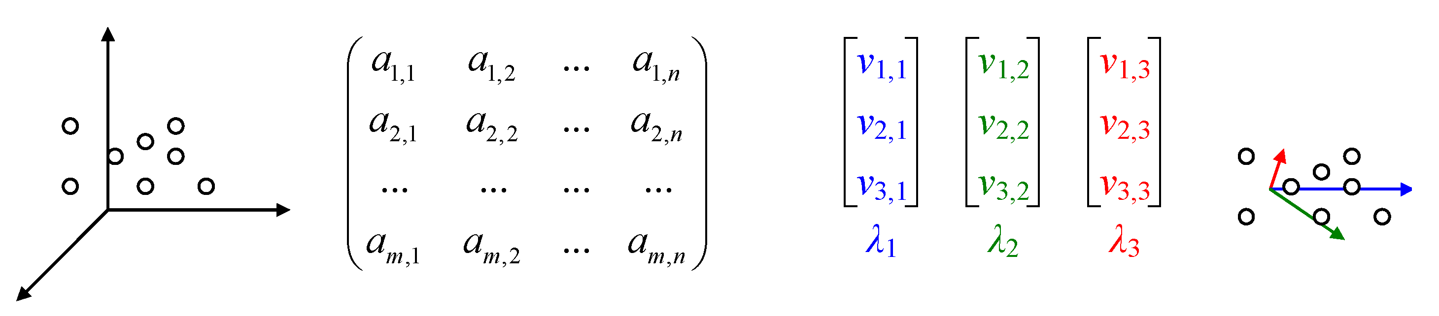
Eigenvalues and eigenvectors are special quantities when related to their precursor entities. One can imagine that the usual space is replaced by another space—eigenspace (Figure 1).

Figure 1. Euclidean space and data (left) vs. Eigenspace and features (right).

The properties of eigenvalues on orthogonal matrices were studied in [72], on skew-symmetric matrices in [73], and on anti-symmetric matrices in [74]. An explicit solution to the eigenvalue problem of a self-adjoint differential operator with a given set of self-adjoint boundary conditions (in terms of the Green’s function, eigenfunctions, and eigenvalues of another problem having the same operator but different boundary conditions) is provided as an extension of the Sturm–Liouville theory in [75].

The method of transplantation was proposed in [76] to be applied if the functional in question is characterized as the extremum value of another functional over a certain function class with respect to the domain of definition. The method was later applied in the theory of torsional rigidity, virtual mass, and conformai radius [76], in the case of the membrane equation and a general problem of electrostatic capacity of a body with a boundary surface and an exterior [77]. Poisson’s equation on complete noncompact manifolds with nonnegative Ricci curvature is tackled in [78], and eigenvalues for integral operators in [79]. Random Hermitian matrices, of interest in statistical physics, also reveal peculiar eigenvalue sets in connection with the distribution of prime numbers [80,81,82].

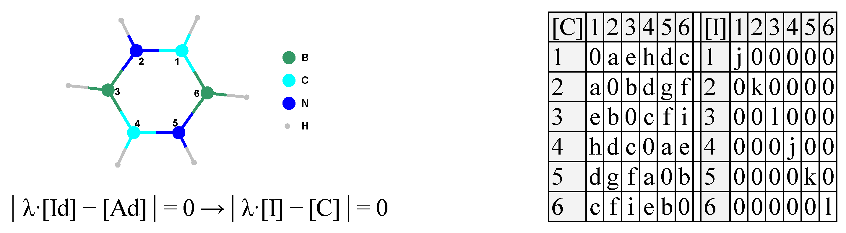
Undirected and unweighted graphs are just a case often used in molecular sciences [15], and an adjacency matrix, square and symmetric, is the scholastic example (Figure 2), possessing a series of important properties [83].

Figure 2. From graphs to molecules by generalizing the adjacency and identity matrices.

One important consequence of operating on integer-based matrices is the possibility of extracting the exact values of the characteristic polynomial coefficients one by one (Algorithm 1, Ref. [84]). This, when coupled with a polynomial root finder algorithm [85], becomes a powerful tool for eigenvalue finding [86]. The difference between extreme eigenvalues of a graph is commonly referred to as the spread of the graph [87].

6. Classical Case Studies

Eigenproblems appear in:

• Quantum localization: quantum theory states that the energy levels correspond to the eigenvalues of a Scrödinger operator [88]; when the operator is too complex, it is often replaced by a random Hermitian matrix and its eigenvalues should correspond to the energy levels of the system; the Gaussian orthogonal ensemble and Gaussian unitary ensemble are typical examples of specific instances [89]; quantum mechanics for particle localization [90], quantification of energy [91], magnetic momentum [92], and electronic spin [93], and the complementary problem of geometrical alignment with complex eigenvalues [74];
• Molecular topology [94] utilizes so-called molecular graphs, which use graph theory to operate on molecular structures. Characterizing molecular graphs is a matter of whether a graph has a certain property. The adjacency matrix $A\left(A_{i,j}\right)$ with entries of 1 if i and j are connected by an edge, otherwise 0. The distance matrix is an extension of it. Another extension is by considering counts of the number of edges for multiple edges and negative integers for directed graphs. In all instances, a characteristic polynomial can be built [15];
• Vibrations of bars and strings [95], and more general to wave propagation [96];
• Laplace’s equation (and its generalizations, Poisson and Helmholtz’s equations), or the potential theory of harmonic functions, in problems involving electrostatic fields, heat conduction, shapes of films and membranes, gravitation and hydrodynamics [97];
• The Sturm–Liouville problem [98], with particular cases to Bessel and Legendre’s equations and the complementary problem of nuclear collisions with complex eigenvalues [99];
• Stability analysis of systems characterized by sets of ordinary differential equations [100];
• Electrical circuits emulating eigenproblems [101].

7. Applications

Matrices of quaternions [102] require special treatment regarding the eigenvalues. Actually, there are two eigenproblems to be solved, left ($Ax=\lambda x$, [103]) and right ($Ax=x\lambda$, [104]). The right eigenproblem has its solutions invariant under the similar transformation [105].

Spectral decomposition uses eigenvalues [106] and is involved in the analysis of variance. For the covariance matrix of the errors, see [107]. For the variability of a tensor-valued random variable, see [108]. For Lamb waves decomposition, see [109]. For nonparametric forecasting of data, see [110]. The fact that the state of a bilinear control system can be split uniquely into generalized modes corresponding to the eigenvalues of the dynamics matrix is proven in [106].

In electric circuits, high impedance faults can be identified by inspecting the eigenvalue space of the circuit [111]. Thus, stability analysis can rely on the calculation of the eigenvalues [112]. The stability of different systems is inspected this way: wind turbines in [113], fluids with non-parallel flow in [114], impedance- and admittance-based electrical systems in [115], three-wheel vehicles in [116], and polynomially dependent one-parameter systems in general in [117].

Classical multivariate analysis considers vectors $v\in {\mathbb{R}}^m$, such that for all $u\in {\mathbb{R}}^m$, $u^{T}v$ is a univariate normal, while v establishes the m-variate normal distribution with $\mu \leftarrow E\left(v\right)$ as mean and $\mathsf{\Sigma }=E\left((v-\mu ){(v-\mu )}^T\right)$ as covariance. The Wishart matrix $W\leftarrow A^{T}A$, computed from an n by m matrix, A, collecting n samples, defines the Wishart distribution. An important property of the Wishart distribution is that it is the sampling distribution of the maximum likelihood estimator (MLE) of the covariance matrix of a multivariate normal distribution [118]. Eigenvalues of a matrix are informative about matrix structure, thus the eigenvalues of the sample covariance matrices give information about the underlying distribution [119].

Principal component analysis (PCA, [120]) is a way of identifying patterns in data, and expressing the data in such a way so as to highlight their similarities and differences. In doing so, it reduces the dimensionality of a data set based on calculating eigenvectors and eigenvalues of the input data (Algorithm 9).

Algorithm 9 First Principal Component

Input: A    //a data matrix with zero mean, A  procedure FPC($A,c,B$)     $x\leftarrow \text{RAND}$; $x\leftarrow \mathrm{U}\text{NIT}\mathrm{V}\left(x\right)$    // Random initialization     For $(j=0;j<\mathrm{C}\text{OLS}(A);j\leftarrow j+1)$    //For each column of data        $y\leftarrow 0$; For $(i=0;i<\mathrm{R}\text{OWS}(A);i\leftarrow i+1)y\leftarrow y+\left(A\right[i\left]x\right)A\left[i\right]$ EndFor        $c\leftarrow x^{T}y$; $x\leftarrow \mathrm{U}\text{NIT}\mathrm{V}\left(y\right)$; If($\mathrm{A}\text{BS}(cx-y)<ϵ$) $\mathrm{E}\text{XIT}$     EndFor  end procedure     $\mathrm{CPC}(A,c,B)$    // B is the first principal component Output: $c,B$    // eigenvalue and its eigenvector

Once the first component is extracted, the algorithm (Algorithm 9) can easily be adapted to extract the rest of the components.

Dominant component analysis is a PCA variation meant to extract an orthogonal set of data descriptors in relation to an dependent variable [121]. Discriminant component analysis is a PCA variation provided as a feature extraction scheme for face recognition [122]. Factor analysis is another variation from PCA designed to identify certain unobservable factors from the observed variables [123]. In PCA, one rewrites the samples on the basis of the eigenvectors. The components of the vector so formed are the principal components and their variances are eigenvalues [124]. In data of high dimensions, where the luxury of graphical representation is not available, PCA is a powerful tool for analyzing data. Another use of PCA is for data compressing: once patterns in data are identified, reducing the number of dimensions without much loss of information is possible.

Image compression [125], denoising [126], and recognition [127] perform eigenvector decomposition, which is very useful in computer tomography [128], magnetic resonance [129], and polarized light [130] imaging, stratigraphic mapping [131], lidar [132], and radar [133].

Principal component regression ([134], PCR) is a regression based on PCA in which the principal components of the explanatory variables are used as regressors. In some instances, large sets of independent variables are available (7 in [135], 13 in [136], 4536 in [88], 576,288 in [15], a maximum number of 787,968 in [137,138,139], or even 2,387,280 in [140,141]. One of the strategies of deriving models for the dependent variable(s) is to perform a full (preferred in [15,137]), heuristic (preferred in [138,139]), random (preferred in [140]), or combined (preferred in [141]) search, while other approaches extract principal components from the pool of independent variables (preferred in [135,136]) and, in other instances, grouping and classification based on the principal components is desired (as in [88]).

Quantum localization is, in the end, a problem of optimization. A less-known fact is that the BFGS (from Broyden, Fletcher, Goldfarb, and Shanno, see [142,143,144,145]) algorithm, as well as other built-in algorithms for quantum localization, such as the DFP (from Davidon, Fletcher, and Powell, see [146,147,148]) and the steepest descent method [149], are closely related to the calculation of the eigenvalues [150]. Several recent modifications [151,152,153,154] make them even more versatile in unconstrained nonlinear optimization.

8. Conclusions and Perspectives

Eigenproblem basics and algorithms are revised from a historical perspective. Many problems may be formulated as eigenproblems, and both classical cases as well as many other discovered applications contain a large pool of variate uses. Several classical eigenvalue and eigenvector calculation algorithms are given and their use is exemplified.

More and more eigenproblem algorithms are stated every day. In [155], the authors propose selection procedures that improve spectral clustering algorithms in high-dimensional settings. The use of a trimmed sampling algorithm applied on the eigenvalues is proposed in [156] to replace the iterated eigenvalues for localization problems of large quantum systems. In [157], an iterative algorithm is proposed for the extraction of analytic eigenvectors for decomposition of parahermitian matrices arising in broadband multiple-input multiple-output systems or array processing.

References

- Euler, L. Du mouvement d’un corps solide quelconque lorsqu’il tourne autour d’un axe mobile. Hist. L’académie R. Des Sci. Belles Lettres Berl. 1767, 1760, 176–227. [Google Scholar]
- Lagrange, J. Nouvelle solution du problème du mouvement de rotation d’un corps de figure quelconque qui n’est animé par aucune force accélératrice. Nouv. Mem. L’académie Sci. Berl. 1775, 1773, 577–616. [Google Scholar]
- Laplace, L. Mémoire sur les solutions particulières des équations différentielles et sur les inégalités séculaires des planètes. Mém. L’académie Sci. Paris 1775, 1775, 325–366. [Google Scholar]
- Fourier, J. Thèorie Analytique de la Chaleur; Firmin Didiot: Paris, France, 1822; pp. 99–427. [Google Scholar]
- Cauchy, A. Sur 1’équation à l’aide de laquelle on determine les inégalités séculaires des mouvements des planètes. Ex. Math. 1829, 4, 174–195. [Google Scholar]
- Sylvester, J. Additions to the articles, “On a new class of theorems”, and “On Pascal’s theorem”. Philos. Mag. 1850, 37, 363–370. [Google Scholar] [CrossRef][Green Version]
- Hermite, C. Sur l’extension du théorème de M. Sturm a un système d’équations simultanées. C. R. Séances Acad. Sci. 1852, 35, 133. [Google Scholar]
- Sylvester, J. On the theorem connected with Newton’s rule for the discovery of imaginary roots of equations. Messenger Math. 1880, 9, 71–84. [Google Scholar]
- Golub, G.H.; van der Vorst, H.A. Eigenvalue computation in the 20th century. J. Comput. Appl. Math. 2000, 123, 35–65. [Google Scholar] [CrossRef]
- Jäntschi, L. Binomial Distributed Data Confidence Interval Calculation: Formulas, Algorithms and Examples. Symmetry 2022, 14, 1104. [Google Scholar] [CrossRef]
- Kronecker, L. Die Periodensysteme von Functionen reeller Variabein. Monatsberichte Der KöNiglich Prenssischen Akad. Der Wiss. Berl. 1884, 11, 1071–1080. [Google Scholar]
- Carlson, D. On real eigenvalues of complex matrices. Pac. J. Math. 1965, 15, 1119–1129. [Google Scholar] [CrossRef]
- Picinbono, B. On circularity. IEEE Trans. Signal Process. 1994, 42, 3473–3482. [Google Scholar] [CrossRef]
- Massey, S.; Zoellner, R.W. MNDO calculations on borazine derivatives. 2. Substitution of two [HNBH] fragments for two [HCCH] fragments in benzene to form the diazadiborines and the novel open structure of the 1,2,4,5-isomer. Inorg. Chem. 1991, 30, 1063–1066. [Google Scholar] [CrossRef]
- Joiţa, D.M.; Jäntschi, L. Extending the characteristic polynomial for characterization of C20 fullerene congeners. Mathematics 2017, 5, 84. [Google Scholar] [CrossRef]
- Brualdi, R. The Jordan canonical form: An old proof. Am. Math. Mon. 1987, 94, 257–267. [Google Scholar] [CrossRef]
- Le Verrier, U. Sur les variations séculaires des éléments des orbites pour les sept planètes principales: Mercure, Vénus, La Terre, Mars, Jupiter, Saturne et Uranus. J. Math. 1840, 5, 220–254. [Google Scholar]
- Jenkins, M. Algorithm 493: Zeros of a real polynomial [C2]. ACM Trans. Math. Softw. 1975, 1, 178–189. [Google Scholar] [CrossRef]
- Sharma, J.; Kumar, S.; Jäntschi, L. On a class of optimal fourth order multiple root solvers without using derivatives. Symmetry 2019, 11, 1452. [Google Scholar] [CrossRef]
- Kumar, S.; Kumar, D.; Sharma, J.; Cesarano, C.; Agarwal, P.; Chu, Y.M. An optimal fourth order derivative-free numerical algorithm for multiple roots. Symmetry 2020, 12, 1038. [Google Scholar] [CrossRef]
- Von Mises, R.; Pollaczek-Geiringer, H. Praktische Verfahren der Gleichungsauflösung. Z. Angew. Math. Mech. 1929, 9, 152–164. [Google Scholar] [CrossRef]
- Clasen, B. Sur une nouvelle méthode de résolution des équations linéaires et sur l’application de cette méthode au calcul des déterminants. Ann. Soc. Sci. Bruxelles 1888, 12, 251–281. [Google Scholar]
- Pohlhausen, E. Berechnung der Eigenschwingungen statisch-bestimmter Fachwerke. Z. Angew. Math. Mech. 1921, 1, 28–42. [Google Scholar] [CrossRef]
- Ritz, W. Über eine neue Methode zur Lösung gewisser Variationsprobleme der mathematischen Physik. J. Reine Angew. Math. 1909, 135, 1–61. [Google Scholar] [CrossRef]
- Ipsen, I. Computing an eigenvector with inverse iteration. SIAM Rev. 1997, 39, 254–291. [Google Scholar] [CrossRef]
- Lanczos, C. An iteration method for the solution of the eigenvalue problem of linear differential and integral operators. J. Res. Natl. Bur. Stand. 1950, 45, 255–282. [Google Scholar] [CrossRef]
- Arnoldi, W. The principle of minimized iteration in the solution of the matrix eigenvalue problem. Quart. Appl. Math. 1951, 9, 17–29. [Google Scholar] [CrossRef]
- Paige, C.C.; Saunders, M.A. Solution of sparse indefinite systems of linear equations. SIAM J. Numer. Anal. 1975, 12, 617–629. [Google Scholar] [CrossRef]
- Saad, Y. Krylov subspace methods for solving large unsymmetric linear systems. Math. Comp. 1981, 37, 105–126. [Google Scholar] [CrossRef]
- Saad, Y.; Schultz, M.H. GMRES: A generalized minimal residual algorithm for solving nonsymmetric linear systems. SIAM J. Sci. Stat. Comput. 1986, 7, 856–869. [Google Scholar] [CrossRef]
- Krylov, A.N. O čislennom rešenii uravnenija, kotorym v tehničeskih voprosah opredeljajutsja častoty malyh kolebanij material’nyh sistem. Izv. Akad. Nauk. SSSR Sci. Math. Natl. 1931, 7, 491–539. [Google Scholar]
- Schmidt, E. Zur Theorie der linearen und nichtlinearen Integralgleichungen I. Teil: Entwicklung willkürlicher Funktionen nach Systemen vorgeschriebener. Math. Ann. 1907, 63, 433–476. [Google Scholar] [CrossRef]
- Hessenberg, K. Behandlung linearer Eigenwertaufgaben mit Hilfe der Hamilton-Cayleyschen Gleichung. Num. Verf. Inst. Prakt. Math. Tech. Hochs. Darmstadt 1907, 63, 1–36. [Google Scholar]
- Da Fonseca, C.M. On the eigenvalues of some tridiagonal matrices. J. Comput. Appl. Math. 2007, 200, 283–286. [Google Scholar] [CrossRef]
- Morgan, R.B. Computing interior eigenvalues of large matrices. Linear Algebra Appl. 1991, 154–156, 289–309. [Google Scholar] [CrossRef]
- Terao, T. Computing interior eigenvalues of nonsymmetric matrices: Application to three-dimensional metamaterial composites. Phys. Rev. E Stat. Nonlin. Soft Matter Phys. 2010, 82, 026702. [Google Scholar] [CrossRef]
- Petrenko, T.; Rauhut, G. A new efficient method for the calculation of interior eigenpairs and its application to vibrational structure problems. J. Chem. Phys. 2017, 146, 124101. [Google Scholar] [CrossRef]
- Jamalian, A.; Aminikhah, H. A novel algorithm for computing interior eigenpairs of large non-symmetric matrices. Soft Comput. 2021, 25, 11865–11876. [Google Scholar] [CrossRef]
- Morgan, R.B.; Zeng, M. Harmonic projection methods for large non-symmetric eigenvalue problems. Numer. Linear Algebra Appl. 1998, 5, 33–55. [Google Scholar] [CrossRef]
- Asakura, J.; Sakurai, T.; Tadano, H.; Ikegami, T.; Kimura, K. A numerical method for polynomial eigenvalue problems using contour integral. Jpn. J. Indust. Appl. Math. 2010, 27, 73–90. [Google Scholar] [CrossRef]
- Stor, N.J.; Slapničar, I.; Barlow, J.L. Accurate eigenvalue decomposition of real symmetric arrowhead matrices and applications. Linear Algebra Appl. 2015, 464, 62–89. [Google Scholar] [CrossRef]
- Wang, Q.W.; Wang, X.X. Arnoldi method for large quaternion right eigenvalue problem. J. Sci. Comput. 2020, 82, 58. [Google Scholar] [CrossRef]
- Saibaba, A.; Lee, J.; Kitanidis, P. Randomized algorithms for generalized hermitian eigenvalue problems with application to computing Karhunen-Loéve expansion. Numer. Linear Algebra Appl. 2016, 23, 314–339. [Google Scholar] [CrossRef]
- Sorensen, D.C. Implicit application of polynomial filters in a k-step Arnoldi method. SIAM J. Matrix Anal. Appl. 1992, 13, 357–385. [Google Scholar] [CrossRef]
- Świrydowicz, K.; Langou, J.; Ananthan, S.; Yang, U.; Thomas, S. Low synchronization Gram–Schmidt and generalized minimal residual algorithms. Numer. Linear Algebra Appl. 2021, 28, e2343. [Google Scholar] [CrossRef]
- Chen, J.; Rong, Y.; Zhu, Q.; Chandra, B.; Zhong, H. A generalized minimal residual based iterative back propagation algorithm for polynomial nonlinear models. Syst. Control Lett. 2021, 153, 104966. [Google Scholar] [CrossRef]
- Jadoui, M.; Blondeau, C.; Martin, E.; Renac, F.; Roux, F.X. Comparative study of inner–outer Krylov solvers for linear systems in structured and high–order unstructured CFD problems. Comput. Fluids 2022, 244, 105575. [Google Scholar] [CrossRef]
- Choi, M.D.; Huang, Z.; Li, C.K.; Sze, N.S. Every invertible matrix is diagonally equivalent to a matrix with distinct eigenvalues. Linear Algebra Appl. 2012, 436, 3773–3776. [Google Scholar] [CrossRef]
- Cayley, A. Sur quelques propriétés des déterminants gauches. J. Reine Angew. Math. 1846, 32, 119–123. [Google Scholar] [CrossRef]
- Meerbergen, K.; Spence, A.; Roose, D. Shift-invert and Cayley transforms for detection of rightmost eigenvalues of nonsymmetric matrices. BIT Numer. Math. 1994, 34, 409–423. [Google Scholar] [CrossRef]
- Benoit, E. Note sur une méthode de résolution des équations normales provenant de l’application de la méthode des moindres carrés à un systéme d’équations linéaires en nombre inférieur à celui des inconnues (Procédé du Commandant Cholesky). Bull. Géodésique 1924, 2, 66–77. [Google Scholar] [CrossRef]
- Schmid, E. An iterative procedure to compute the modal matrix of eigenvectors. J. Geophys. Res. 1971, 76, 1916–1920. [Google Scholar] [CrossRef]
- Saad, Y. Chebyshev acceleration techniques for solving nonsymmetric eigenvalue problems. Math. Comp. 1984, 42, 567–588. [Google Scholar] [CrossRef]
- Saad, Y. Numerical solution of large nonsymmetric eigenvalue problems. Comput. Phys. Commun. 1989, 53, 71–90. [Google Scholar] [CrossRef][Green Version]
- Duff, I.S.; Scott, J.A. Computing selected eigenvalues of large sparse unsymmetric matrices using subspace iteration. ACM Trans. Math. Softw. 1993, 19, 137–159. [Google Scholar] [CrossRef]
- Chebyshev, P. Théorie des mécanismes connus sous le nom de parallélogrammes. Mém. Savants Étr. Acad. Saint-Pétersbourg 1854, 7, 539–586. [Google Scholar]
- Horning, A.; Nakatsukasa, Y. Twice is enough for dangerous eigenvalues. SIAM J. Matrix Anal. Appl. 2022, 43, 68–93. [Google Scholar] [CrossRef]
- Davidson, E. The iterative calculation of a few of the lowest eigenvalues and corresponding eigenvectors of large real-symmetric matrices. J. Comp. Phys. 1975, 17, 87–94. [Google Scholar] [CrossRef]
- Jacobi, C. Über ein leichtes Verfahren die in der Theorie der Säacularstörungen vorkommenden Gleichungen numerisch aufzulöosen. J. Reine Angew. Math. 1846, 30, 51–95. [Google Scholar] [CrossRef]
- Sleijpen, G.; Van Der Vorst, H. A Jacobi–Davidson iteration method for linear eigenvalue problems. SIAM J. Matrix Anal. Appl. 1996, 17, 401–425. [Google Scholar] [CrossRef]
- Sleijpen, G.; Van Der Vorst, H. A Jacobi–Davidson iteration method for linear eigenvalue problems. SIAM Rev. Soc. Ind. Appl. Math. 2000, 42, 267–293. [Google Scholar] [CrossRef]
- Hochstenbach, M.; Notay, Y. The Jacobi–Davidson method. GAMM-Mitteilungen 2006, 29, 368–382. [Google Scholar] [CrossRef]
- Seidel, L. Über ein Verfahren, die Gleichungen, auf welche die Methode der kleinsten Quadrate führt, sowie lineäre Gleichungen überhaupt, durch successive Annäherung aufzulösen. Abh. Math.-Phys. Kl. K. Bayer. Akad. Wiss. 1874, 11, 81–108. [Google Scholar]
- Urekew, T.; Rencis, J. The importance of diagonal dominance in the iterative solution of equations generated from the boundary element method. Int. J. Numer. Meth. Engng. 1993, 36, 3509–3527. [Google Scholar] [CrossRef]
- Francis, J.G.F. The QR transformation, I. Comput. J. 1961, 4, 265–271. [Google Scholar] [CrossRef]
- Francis, J.G.F. The QR transformation, II. Comput. J. 1962, 4, 332–345. [Google Scholar] [CrossRef]
- Kublanovskaya, V.N. O nekotorykh algorifmakh dlya resheniya polnoy problemy sobstvennykh znacheniy. Zh. Vychisl. Mat. Mat. Fiz. 1961, 1, 555–570. [Google Scholar]
- Kublanovskaya, V.N. On some algorithms for the solution of the complete eigenvalue problem. USSR Comput. Math. Math. Phys. 1962, 1, 637–657. [Google Scholar] [CrossRef]
- Watkins, D. Francis’s Algorithm. Am. Math. Mon. 2011, 118, 387–403. [Google Scholar] [CrossRef]
- Demmel, J.; Grigori, L.; Hoemmen, M.; Langou, J. Communication-optimal parallel and sequential QR and LU factorizations. arXiv 2008, arXiv:0806.2159. [Google Scholar] [CrossRef]
- Fahey, M. Algorithm 826: A parallel eigenvalue routine for complex Hessenberg matrices. ACM Trans. Math. Softw. 2003, 29, 326–336. [Google Scholar] [CrossRef]
- Schwerdtfeger, H. On the Representation of Rigid Rotations. J. Appl. Phys. 1945, 16, 571–576. [Google Scholar] [CrossRef]
- Drazin, M. A Note on Skew-Symmetric Matrices. Math. Gaz. 1952, 36, 253–255. [Google Scholar] [CrossRef]
- Jäntschi, L. The Eigenproblem Translated for Alignment of Molecules. Symmetry 2019, 11, 1027. [Google Scholar] [CrossRef]
- Weinberger, H. An extension of the classical Sturm-Liouville theory. Duke Math. J. 1955, 22, 1–14. [Google Scholar] [CrossRef]
- Pólya, G.; Schiffer, M. Convexity of functionals by transplantation. J. Anal. Math. 1953, 3, 245–345. [Google Scholar] [CrossRef]
- Schiffer, M. Variation of domain functionals. Bull. Amer. Math. Soc. 1954, 60, 303–328. [Google Scholar] [CrossRef]
- Ni, L.; Shi, Y.; Tam, L. Poisson Equation, Poincaré-Lelong Equation and Curvature Decay on Complete Kähler Manifolds. J. Differential Geom. 2001, 57, 339–388. [Google Scholar] [CrossRef]
- Karlin, S. The existence of eigenvalues for integral operators. Trans. Amer. Math. Soc. 1964, 113, 1–17. [Google Scholar] [CrossRef]
- Montgomery, H. The Pair Correlation of Zeros of the Zeta Function. Proc. Sympos. Pure Math. 1973, 24, 181–193. [Google Scholar] [CrossRef]
- Odlyzko, A. On the distribution of spacings between zeros of zeta functions. Math. Comp. 1987, 48, 273–308. [Google Scholar] [CrossRef]
- Katz, N.; Sarnak, P. Zeroes of zeta functions and symmetry. Bull. Amer. Math. Soc. 1999, 36, 1–26. [Google Scholar] [CrossRef]
- D’Amato, S.; Gimarc, B.; Trinajstić, N. Isospectral and subspectral molecules. Croat. Chem. Acta. 1981, 54, 1–52. [Google Scholar]
- Bolboacă, S.; Jäntschi, L. Characteristic Polynomial in Assessment of Carbon-Nano Structures. In Sustainable Nanosystems Development, Properties, and Applications; Putz, M., Mirică, M., Eds.; IGI Global: Hershey, PA, USA, 2017. [Google Scholar] [CrossRef]
- Jenkins, M.; Traub, J. Algorithm 419: Zeros of a complex polynomial [C2]. Commun. ACM 1972, 15, 97–99. [Google Scholar] [CrossRef]
- Jäntschi, L.; Bolboacă, S. Characteristic polynomial. In New Frontiers in Nanochemistry: Concepts, Theories, and Trends; Putz, M., Ed.; Apple Academic Press: New York, NY, USA, 2020; Volume 2. [Google Scholar] [CrossRef]
- Fan, Y.Z.; Xu, J.; Wang, Y.; Liang, D. The Laplacian spread of a tree. Discret. Math. Theor. Comput. Sci. 2008, 10, 79–86. [Google Scholar] [CrossRef]
- Bálint, D.; Jäntschi, L. Comparison of Molecular Geometry Optimization Methods Based on Molecular Descriptors. Mathematics 2021, 9, 2855. [Google Scholar] [CrossRef]
- Pandey, A.; Mehta, M. Gaussian ensembles of random hermitian matrices intermediate between orthogonal and unitary ones. Commun. Math. Phys. 1983, 87, 449–468. [Google Scholar] [CrossRef]
- Pauli, W. Relativistic Field Theories of Elementary Particles. Rev. Mod. Phys. 1941, 13, 203–232. [Google Scholar] [CrossRef]
- Schrödinger, E. A Method of Determining Quantum-Mechanical Eigenvalues and Eigenfunctions. Proc. R. Irish Acad. A Math. Phys. Sci. 1941, 46, 9–16. [Google Scholar]
- Pryce, M. The Eigenvalues of Electromagnetic Angular Momentum. Math. Proc. Camb. Philos. Soc. 1936, 32, 614–621. [Google Scholar] [CrossRef]
- Landé, A. Eigenvalue Problem of the Dirac Electron. Phys. Rev. 1940, 57, 1183–1184. [Google Scholar] [CrossRef]
- Diudea, M.; Gutman, I.; Jäntschi, L. Molecular Topology; Nova Science: New York, NY, USA, 2001. [Google Scholar]
- Babuška, I.; Osborn, J. Eigenvalue problems. Handb. Numer. Anal. 1991, 2, 641–787. [Google Scholar] [CrossRef]
- MacFarlane, G. A variational method for determining eigenvalues of the wave equation applied to tropospheric refraction. Math. Proc. Camb. Philos. Soc. 1947, 43, 213–219. [Google Scholar] [CrossRef]
- Shortley, G.; Weller, R. The Numerical Solution of Laplace’s Equation. J. Appl. Phys. 1938, 9, 334–344. [Google Scholar] [CrossRef]
- Freilich, G. Note on the eigenvalues of the Sturm-Liouville differential equation. Bull. Am. Math. Soc. 1948, 54, 405–408. [Google Scholar] [CrossRef]
- Peierls, R. Expansions in terms of sets of functions with complex eigenvalues. Math. Proc. Camb. Philos. Soc. 1948, 44, 242–250. [Google Scholar] [CrossRef]
- Flower, J.; Parr, E. Control Systems. In Electrical Engineer’s Reference Book, 16th ed.; Elsevier: Oxford, UK, 2003; p. 13. [Google Scholar] [CrossRef]
- Many, A.; Meiboom, S. An electrical network for determining the eigenvalues and eigenvectors of a real symmetric matrix. Rev. Sci. Instr. 1947, 18, 831–836. [Google Scholar] [CrossRef]
- Zhang, F. Quaternions and matrices of quaternions. Linear Algebra Appl. 1997, 251, 21–57. [Google Scholar] [CrossRef]
- Jiang, T.; Chen, L. An algebraic method for Schrödinger equations in quaternionic quantum mechanics. Comput. Phys. Commun. 2008, 178, 795–799. [Google Scholar] [CrossRef]
- Farenick, D.; Pidkowich, B. The spectral theorem in quaternions. Linear Algebra Appl. 2003, 371, 75–102. [Google Scholar] [CrossRef]
- Jia, Z.; Wei, M.; Zhao, M.; Chen, Y. A new real structure-preserving quaternion QR algorithm. J. Comput. Appl. Math. 2018, 343, 26–48. [Google Scholar] [CrossRef]
- Iskakov, A.; Yadykin, I. On Spectral Decomposition of States and Gramians of Bilinear Dynamical Systems. Mathematics 2021, 9, 3288. [Google Scholar] [CrossRef]
- Wansbeek, T.; Kapteyn, A. A simple way to obtain the spectral decomposition of variance components models for balanced data. Commun. Stat. Theory Methods 1982, 11, 2105–2112. [Google Scholar] [CrossRef]
- Basser, P.; Pajevic, S. Spectral decomposition of a 4th-order covariance tensor: Applications to diffusion tensor MRI. Signal Process. 2007, 87, 220–236. [Google Scholar] [CrossRef]
- Pagneux, V.; Maurel, A. Determination of Lamb mode eigenvalues. J. Acoust. Soc. Am. 2001, 110, 1307–1314. [Google Scholar] [CrossRef] [PubMed]
- Giannakis, D. Data-driven spectral decomposition and forecasting of ergodic dynamical systems. Appl. Comput. Harmon. Anal. 2019, 47, 338–396. [Google Scholar] [CrossRef]
- Paramo, G.; Bretas, A. WAMs based eigenvalue space model for high impedance fault detection. Appl. Sci. 2021, 11, 12148. [Google Scholar] [CrossRef]
- Angelidis, G.; Semlyen, A. Improved methodologies for the calculation of critical eigenvalues in small signal stability analysis. IEEE Trans. Power Syst. 1996, 11, 1209–1217. [Google Scholar] [CrossRef]
- Hansen, M. Aeroelastic stability analysis of wind turbines using an eigenvalue approach. Wind Energ. 2004, 7, 133–143. [Google Scholar] [CrossRef]
- Morzyński, M.; Afanasiev, K.; Thiele, F. Solution of the eigenvalue problems resulting from global non-parallel flow stability analysis. Comput. Methods Appl. Mech. Engrg. 1999, 169, 161–176. [Google Scholar] [CrossRef]
- Fan, L.; Miao, Z. Admittance-Based Stability Analysis: Bode Plots, Nyquist Diagrams or Eigenvalue Analysis? IEEE Trans. Power Syst. 2020, 35, 3312–3315. [Google Scholar] [CrossRef]
- Sharma, R. Ride, eigenvalue and stability analysis of three-wheel vehicle using Lagrangian dynamics. Int. J. Vehicle Noise Vib. 2017, 13, 13–25. [Google Scholar] [CrossRef]
- Chen, J.; Fu, P.; Méndez-Barrios, C.; Niculescu, S.I. Zhang, H. Stability Analysis of Polynomially Dependent Systems by Eigenvalue Perturbation. IEEE Trans. Automat. Contr. 2017, 62, 5915–5922. [Google Scholar] [CrossRef]
- Strydom, H.; Crowther, N. Maximum likelihood estimation of parameter structures for the Wishart distribution using constraints. J. Stat. Plan. Inference 2013, 143, 783–794. [Google Scholar] [CrossRef]
- Letac, G.; Massam, H. All Invariant Moments of the Wishart Distribution. Scand. J. Stat. 2004, 31, 295–318. [Google Scholar] [CrossRef]
- Pearson, K. On Lines and Planes of Closest Fit to Systems of Points in Space. Philos. Mag. 1901, 2, 559–572. [Google Scholar] [CrossRef]
- Randić, M. Search for Optimal Molecular Descriptors. Croat. Chem. Acta 1991, 64, 43–54. [Google Scholar]
- Zhao, W. Discriminant component analysis for face recognition. In Proceedings of the 15th International Conference on Pattern Recognition. ICPR-2000, Barcelona, Spain, 3–7 September 2000; Volume 2, pp. 818–821. [Google Scholar] [CrossRef]
- Stephenson, W. Technique of Factor Analysis. Nature 1935, 136, 297. [Google Scholar] [CrossRef]
- Gauch, H. Noise Reduction By Eigenvector Ordinations. Ecology 1982, 63, 1643–1649. [Google Scholar] [CrossRef]
- Claire, E.; Farber, S.M.; Green, R. Practical Techniques for Transform Data Compression/Image Coding. IEEE Trans. Electromagn. Compat. 1971, EMC-13, 2–6. [Google Scholar] [CrossRef]
- Cawley, P.; Adams, R. The location of defects in structures from measurements of natural frequencies. J. Strain. Anal. Eng. Des 1979, 14, 49–57. [Google Scholar] [CrossRef]
- Kim, D.; Ersoy, O. Image recognition with the discrete rectangular-wave transform II. J. Opt. Soc. Am. A 1989, 6, 835–843. [Google Scholar] [CrossRef]
- Sørensen, M. In vivo prediction of goat body composition by computer tomography. Anim. Prod. 1992, 54, 67–73. [Google Scholar] [CrossRef]
- Hasan, K.; Basser, P.; Parker, D.; Alexander, A. Analytical Computation of the Eigenvalues and Eigenvectors in DT-MRI. J. Magn. Reson. 2001, 152, 41–47. [Google Scholar] [CrossRef] [PubMed]
- Jouk, P.; Usson, Y. The Myosin Myocardial Mesh Interpreted as a Biological Analogous of Nematic Chiral Liquid Crystals. J. Cardiovasc. Dev. Dis. 2021, 8, 179. [Google Scholar] [CrossRef] [PubMed]
- Gersztenkorn, A.; Marfurt, K. Eigenstructure-based coherence computations as an aid to 3-D structural and stratigraphic mapping. Geophysics 1999, 64, 1468–1479. [Google Scholar] [CrossRef]
- Si, S.; Hu, H.; Ding, Y.; Yuan, X.; Jiang, Y.; Jin, Y.; Ge, X.; Zhang, Y.; Chen, J.; Guo, X. Multiscale Feature Fusion for the Multistage Denoising of Airborne Single Photon LiDAR. Remote Sens. 2023, 15, 269. [Google Scholar] [CrossRef]
- Shu, G.; Chang, J.; Lu, J.; Wang, Q.; Li, N. A novel method for SAR ship detection based on eigensubspace projection. Remote Sens. 2022, 14, 3441. [Google Scholar] [CrossRef]
- Hotelling, H. The relations of the newer multivariate statistical methods to factor analysis. Brit. J. Stat. Psychol. 1957, 10, 69–79. [Google Scholar] [CrossRef]
- Xiong, Z.; Chen, Y.; Tan, H.; Cheng, Q.; Zhou, A. Analysis of factors influencing the lake area on the Tibetan plateau using an eigenvector spatial filtering based spatially varying coefficient model. Remote Sens. 2021, 13, 5146. [Google Scholar] [CrossRef]
- Liu, S.; Begum, N.; An, T.; Zhao, T.; Xu, B.; Zhang, S.; Deng, X.; Lam, H.M.; Nguyen, H.; Siddique, K.; et al. Characterization of Root System Architecture Traits in Diverse Soybean Genotypes Using a Semi-Hydroponic System. Plants 2021, 10, 2781. [Google Scholar] [CrossRef]
- Jäntschi, L.; Bolboacă, S. Results from the Use of Molecular Descriptors Family on Structure Property/Activity Relationships. Int. J. Mol. Sci. 2007, 8, 189–203. [Google Scholar] [CrossRef]
- Bolboaca, S.D.; Jäntschi, L.; Diudea, M.V. Molecular Design and QSARs/QSPRs with Molecular Descriptors Family. Curr. Comput. Aided Drug Des. 2013, 9, 195–205. [Google Scholar] [CrossRef] [PubMed]
- Jäntschi, L.; Bolboaca, S.; Diudea, M. Chromatographic Retention Times of Polychlorinated Biphenyls: From Structural Information to Property Characterization. Int. J. Mol. Sci. 2007, 8, 1125–1157. [Google Scholar] [CrossRef]
- Bolboacă, S.; Jäntschi, L. Comparison of quantitative structure-activity relationship model performances on carboquinone derivatives. Sci. World J. 2009, 9, 1148–1166. [Google Scholar] [CrossRef]
- Bolboacă, S.; Jäntschi, L. Predictivity Approach for Quantitative Structure-Property Models. Application for Blood-Brain Barrier Permeation of Diverse Drug-Like Compounds. Int. J. Mol. Sci. 2011, 12, 4348–4364. [Google Scholar] [CrossRef]
- Broyden, C. The convergence of a class of double-rank minimization algorithms. J. Inst. Math. Appl. 1970, 6, 76–90. [Google Scholar] [CrossRef]
- Fletcher, R. A New Approach to Variable Metric Algorithms. Comput. J. 1970, 13, 317–322. [Google Scholar] [CrossRef]
- Goldfarb, D. A Family of Variable Metric Updates Derived by Variational Means. Math. Comput. 1970, 24, 23–26. [Google Scholar] [CrossRef]
- Shanno, D. Conditioning of quasi-Newton methods for function minimization. Math. Comput. 1970, 24, 647–656. [Google Scholar] [CrossRef]
- Davidon, W. Variable Metric Method for Minimization. AEC Research and Development Report ANL-5990; Argonne National Laboratory: Lemont, IL, USA, 1959. [Google Scholar]
- Fletcher, R. Practical Methods of Optimization vol. 1: Unconstrained Optimization; John Wiley & Sons: New York, NY, USA, 1987. [Google Scholar] [CrossRef]
- Powell, M. On the convergence of the variable metric algorithm. IMA J. Appl. Math. 1971, 7, 21–36. [Google Scholar] [CrossRef]
- Debye, P. Näherungsformeln für die Zylinderfunktionen für große Werte des Arguments und unbeschränkt veränderliche Werte des Index. Math. Annal. 1909, 67, 535–558. [Google Scholar] [CrossRef]
- Nocedal, J. Theory of algorithms for unconstrained optimization. Acta Numer. 1992, 1, 199–242. [Google Scholar] [CrossRef]
- Neculai, A. A double parameter scaled BFGS method for unconstrained optimization. J. Comput. Appl. Math. 2018, 332, 26–44. [Google Scholar] [CrossRef]
- Liu, Q.; Beller, S.; Lei, W.; Peter, D.; Tromp, J. A double parameter scaled BFGS method for unconstrained optimization. Geophys. J. Int. 2022, 228, 796–815. [Google Scholar] [CrossRef]
- Liang, J.; Shen, S.; Li, M.; Fei, S. Quantum algorithms for the generalized eigenvalue problem. Quantum Inf. Process. 2022, 21, 23. [Google Scholar] [CrossRef]
- Ullah, N.; Shah, A.; Sabi’u, J.; Jiao, X.; Awwal, A.; Pakkaranang, N.; Shah, S.; Panyanak, B. A One-Parameter Memoryless DFP Algorithm for Solving System of Monotone Nonlinear Equations with Application in Image Processing. Mathematics 2023, 11, 1221. [Google Scholar] [CrossRef]
- Han, X.; Tong, X.; Fan, Y. Eigen Selection in Spectral Clustering: A Theory-Guided Practice. J. Am. Stat. Assoc. 2023, 118, 109–121. [Google Scholar] [CrossRef]
- Hicks, C.; Lee, D. Trimmed sampling algorithm for the noisy generalized eigenvalue problem. Phys. Rev. Res. 2023, 5, L022001. [Google Scholar] [CrossRef]
- Weiss, S.; Proudler, I.; Coutts, F.K.; Khattak, F. Eigenvalue Decomposition of a Parahermitian Matrix: Extraction of Analytic Eigenvectors. IEEE Trans. Signal Process. 2023, 71, 1642–1656. [Google Scholar] [CrossRef]
Figure 1.
Euclidean space and data (left) vs. Eigenspace and features (right).
Figure 2.
From graphs to molecules by generalizing the adjacency and identity matrices.