
UAV Dynamic Non-Terrestrial Transmission Channel Analysis Based on SSCM-RT Model

Abstract
:1. Introduction
- A long-distance non-terrestrial transmission channel model for UAVs is established. The channel parameters chosen for the simulation are based on the spatial statistical channel model. To confirm the validity of the SSCM-RT channel model, the path loss simulation results are compared with those from other models.
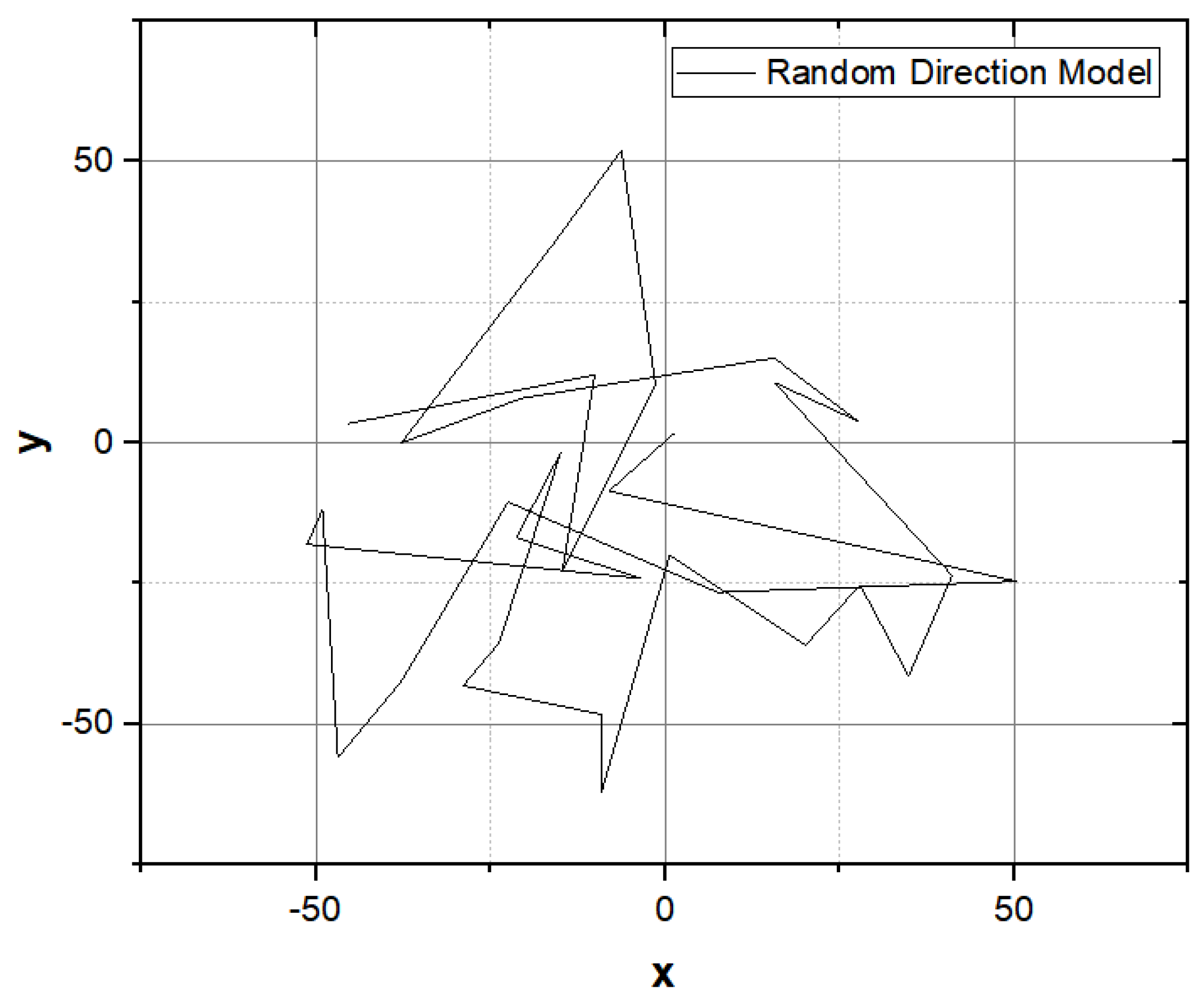
- The relative motion of the UAVs is simulated using various motion models in symmetric and asymmetric scenarios, and the spatial consistency’s impact on the channel is examined. The channel characteristics of several motion models are simulated to further confirm the reliability of the SSCM-RT model.
2. Theoretical Background
2.1. Channel Fading Model Parameters
2.2. Spatial Consistency
3. SSCM-RT Channel Model
3.1. Modeling Scenario Characterization
3.2. SSCM-RT Channel Model Simulation
4. Spatial Consistency of Dynamic Channels
4.1. Spatial Consistency and Motion Models
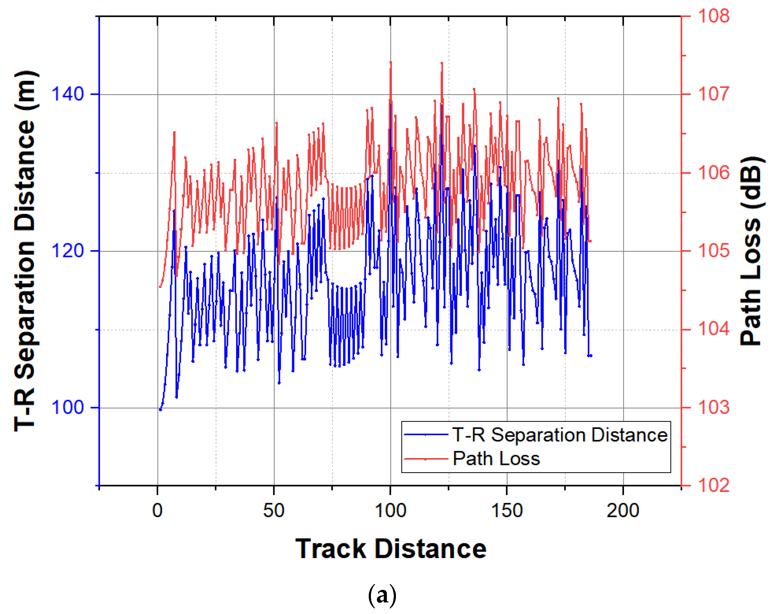
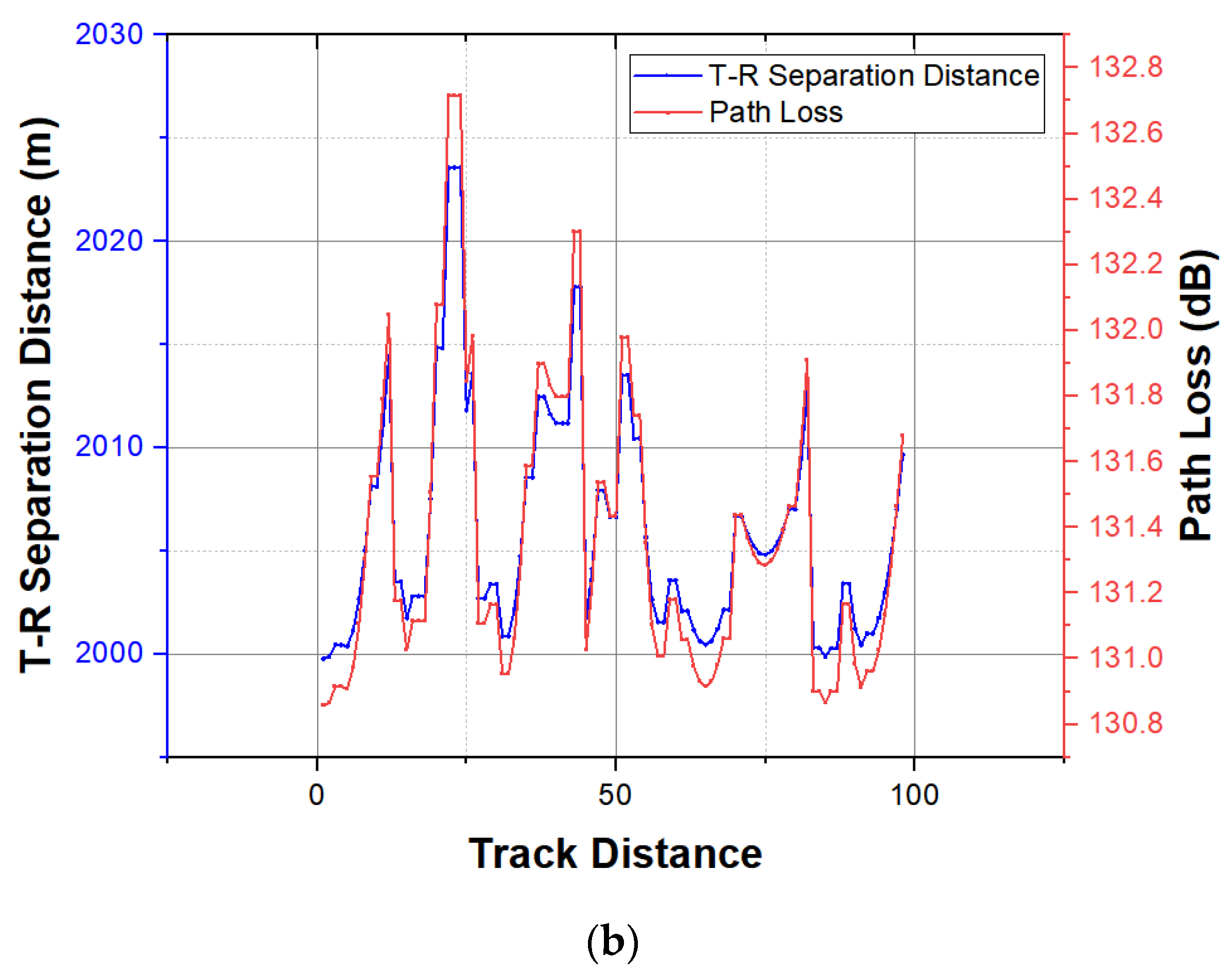
4.2. SSCM-RT Dynamic Channel Simulation
5. Conclusions
Author Contributions
Funding
Data Availability Statement
Conflicts of Interest
Appendix A

| Parameter | Symbol | Description |
|---|---|---|
| T-R Separation Distance (m) | The separation distance from the transmitter (TX) to the receiver (RX). | |
| Time Delay (absolute propagation time) (ns) | The time it takes for an electromagnetic or optical signal to travel a certain distance in the transmission medium. | |
| Received Power (dBm) | The power RX received. | |
| Path Loss (dB) | The loss caused by the propagation of radio waves in space. It is caused by the radiated diffusion of the transmitted power and the propagation characteristics of the channel. | |
| Path Loss Exponent | The path loss exponent ranges from 2 to 6, with 2 representing free space and 6 representing severe obstruction. | |
| Shadow Fading Standard Deviation (dB) | Obstacles attenuate signal power by absorption, reflection, scattering, and diffraction, causing shadow fading. The range is from 5 dB to 12 dB, and the typical value is 8 dB. | |
| TX Ant. HPBW | An editable parameter denoting the azimuth/elevation half-power-beamwidth (HPBW) of the TX antenna (array) in degrees. | |
| TX Ant. Gain (dBi) | TX antenna gain. | |
| RX Ant. HPBW | An editable parameter denoting the azimuth/elevation half-power-beamwidth (HPBW) of the RX antenna (array) in degrees. | |
| RX Ant. Gain (dBi) | RX antenna gain. |
References
- Xiao, Z.; Zhu, L.; Liu, Y.; Yi, P.; Zhang, R.; Xia, X.; Schober, R. A Survey on Millimeter-Wave Beamforming Enabled UAV Communications and Networking. IEEE Commun. Surv. Tutor. 2022, 24, 557–610. [Google Scholar] [CrossRef]
- Bai, L.; Huang, Z.; Zhang, X.; Cheng, X. A Non-Stationary 3D Model for 6G Massive MIMO mmWave UAV Channels. IEEE Trans. Wirel. Commun. 2021, 21, 4325–4339. [Google Scholar] [CrossRef]
- You, X.; Wang, C.-X.; Huang, J.; Gao, X.; Zhang, Z.; Wang, M.; Huang, Y.; Zhang, C.; Jiang, Y.; Wang, J.; et al. Towards 6G wireless communication networks: Vision, enabling technologies, and new pradigm shifts. Sci. China Inf. Sci. 2020, 64, 110301. [Google Scholar] [CrossRef]
- Al-Shammari, B.K.J.; Hburi, I.; Idan, H.R.; Khazaal, H.F. An Overview of mmWave Communications for 5G. In Proceedings of the 2021 International Conference on Communication & Information Technology (ICICT), Basrah, Iraq, 5–6 June 2021; pp. 133–139. [Google Scholar] [CrossRef]
- Bian, J.; Wang, C.-X.; Gao, X.; You, X.; Zhang, M. A General 3D Non-Stationary Wireless Channel Model for 5G and Beyond. IEEE Trans. Wirel. Commun. 2021, 20, 3211–3224. [Google Scholar] [CrossRef]
- Wang, J.; Wang, C.-X.; Huang, J.; Wang, H.; Gao, X. A General 3D Space-Time-Frequency Non-Stationary THz Channel Model for 6G Ultra-Massive MIMO Wireless Communication Systems. IEEE J. Sel. Areas Commun. 2021, 39, 1576–1589. [Google Scholar] [CrossRef]
- Khawaja, W.; Guvenc, I.; Matolak, D.W.; Fiebig, U.-C.; Schneckenburger, N. A Survey of Air-to-Ground Propagation Channel Modeling for Unmanned Aerial Vehicles. IEEE Commun. Surv. Tutor. 2019, 21, 2361–2391. [Google Scholar] [CrossRef]
- Liao, C.; Xu, K.; Xie, W.; Xia, X. 3-D massive MIMO channel model for high-speed railway wireless communication. Radio Sci. 2020, 55, e2020RS007070. [Google Scholar] [CrossRef]
- Sun, S.; Rappaport, T.S.; Heath, R.W.; Nix, A.; Rangan, S. Mimo for millimeter-wave wireless communications: Beamforming, spatial multiplexing, or both? IEEE Commun. Mag. 2014, 52, 110–121. [Google Scholar] [CrossRef]
- Zhu, X. Analysis of military application of UAV swarm technology. In Proceedings of the 2020 3rd International Conference on Unmanned Systems (ICUS), Harbin, China, 27–28 November 2020; pp. 1200–1204. [Google Scholar] [CrossRef]
- Iqbal, A.; Tham, M.; Wong, Y.J.; Al-Habashna, A.; Wainer, G.; Zhu, Y.X.; Dagiuklas, T. Empowering Non-Terrestrial Networks with Artificial Intelligence: A Survey. IEEE Access 2023, 11, 100986–101006. [Google Scholar] [CrossRef]
- Mahboob, S.; Liu, L. Revolutionizing Future Connectivity: A Contemporary Survey on AI-empowered Satellite-based Non-Terrestrial Networks in 6G. arXiv 2023. [Google Scholar] [CrossRef]
- Traspadini, A.; Giordani, M.; Zorzi, M. UAV/HAP-Assisted Vehicular Edge Computing in 6G: Where and What to Offload? In Proceedings of the 2022 Joint European Conference on Networks and Communications & 6G Summit (EuCNC/6G Summit), Grenoble, France, 7–10 June 2022; pp. 178–183. [Google Scholar] [CrossRef]
- Chen, Y.; Li, Y.; Han, C.; Yu, Z.; Wang, G. Channel Measurement and Ray-Tracing-Statistical Hybrid Modeling for Low-Terahertz Indoor Communications. IEEE Trans. Commun. 2021, 20, 8163–8176. [Google Scholar] [CrossRef]
- Luo, W.; Ma, Y.; Shao, X.; Xu, L.; Nan, X. A hybrid near and far−field channel model based on large-scale reconfigurable smart surfaces. J. Electron. Inf. Technol. 2022, 44, 3866–3873. [Google Scholar] [CrossRef]
- Khuwaja, A.A.; Chen, Y.; Zhao, N.; Alouini, M.-S.; Dobbins, P. A Survey of Channel Modeling for UAV Communications. IEEE Commun. Surv. Tutor. 2018, 20, 2804–2821. [Google Scholar] [CrossRef]
- Yang, J.; Li, H.; Xu, Z. Analysis of channel characteristics between satellite and space station in terahertz band based on ray tracing. Radio Sci. 2021, 56, e2021RS007290. [Google Scholar] [CrossRef]
- Yang, J.; Yuan, L. Analysis of channel characteristics for inter-satellite terahertz communication based on Lambertian model. J. Signal Process. 2022, 38, 232–240. [Google Scholar] [CrossRef]
- Rappaport, T.S. Wireless Communications: Principles and Practice; Prentice Hall PTR: Hoboken, NJ, USA, 1996. [Google Scholar]
- Chetlur, V.V.; Dhillon, H.S. Downlink Coverage Analysis for a Finite 3-D Wireless Network of Unmanned Aerial Vehicles. IEEE Trans. Commun. 2017, 65, 4543–4558. [Google Scholar] [CrossRef]
- Mou, M.A.; Mowla, M.M.; Aftabi Momo, S.H. Statistical Channel Model at mmWave Band Inside High Speed Water Vehicle. In Proceedings of the 2019 3rd International Conference on Electrical, Computer & Telecommunication Engineering (ICECTE), Rajshahi, Bangladesh, 26–28 December 2019; pp. 109–112. [Google Scholar] [CrossRef]
- Teixeira, E.; Sousa, S.; Velez, F.J.; Peha, J.M. Impact of the propagation model on the capacity in small-cell networks: Comparison between the UHF/SHF and the millimeter wavebands. Radio Sci. 2021, 56, e2020RS007150. [Google Scholar] [CrossRef]
- Jawhly, T.; Chandra Tiwari, R. Loss exponent modeling for the hilly forested region in the VHF band III. Radio Sci. 2021, 56, e2020RS007201. [Google Scholar] [CrossRef]
- Sun, S.; MacCartney, G.R.; Rappaport, T.S. A novel millimeter-wave channel simulator and applications for 5G wireless communications. In Proceedings of the 2017 IEEE International Conference on Communications (ICC), Paris, France, 21–25 May 2017; pp. 1–7. [Google Scholar] [CrossRef]


| Correlation Distance (m) | Rural Macro | Urban Micro | Urban Macro | Indoor | ||||||
|---|---|---|---|---|---|---|---|---|---|---|
| LOS | NLOS | O2I | LOS | NLOS | O2I | LOS | NLOS | O2I | ||
| Cluster and ray specific random variables | 50 | 60 | 15 | 12 | 15 | 15 | 40 | 50 | 15 | 10 |
| LOS/NLOS state | 60 | 50 | 50 | 10 | ||||||
| Indoor/Outdoor state | 50 | 50 | 50 | N/A | ||||||
| Model | Ray Type | T-R 500 m | T-R 1000 m | T-R 2000 m | T-R 4000 m |
|---|---|---|---|---|---|
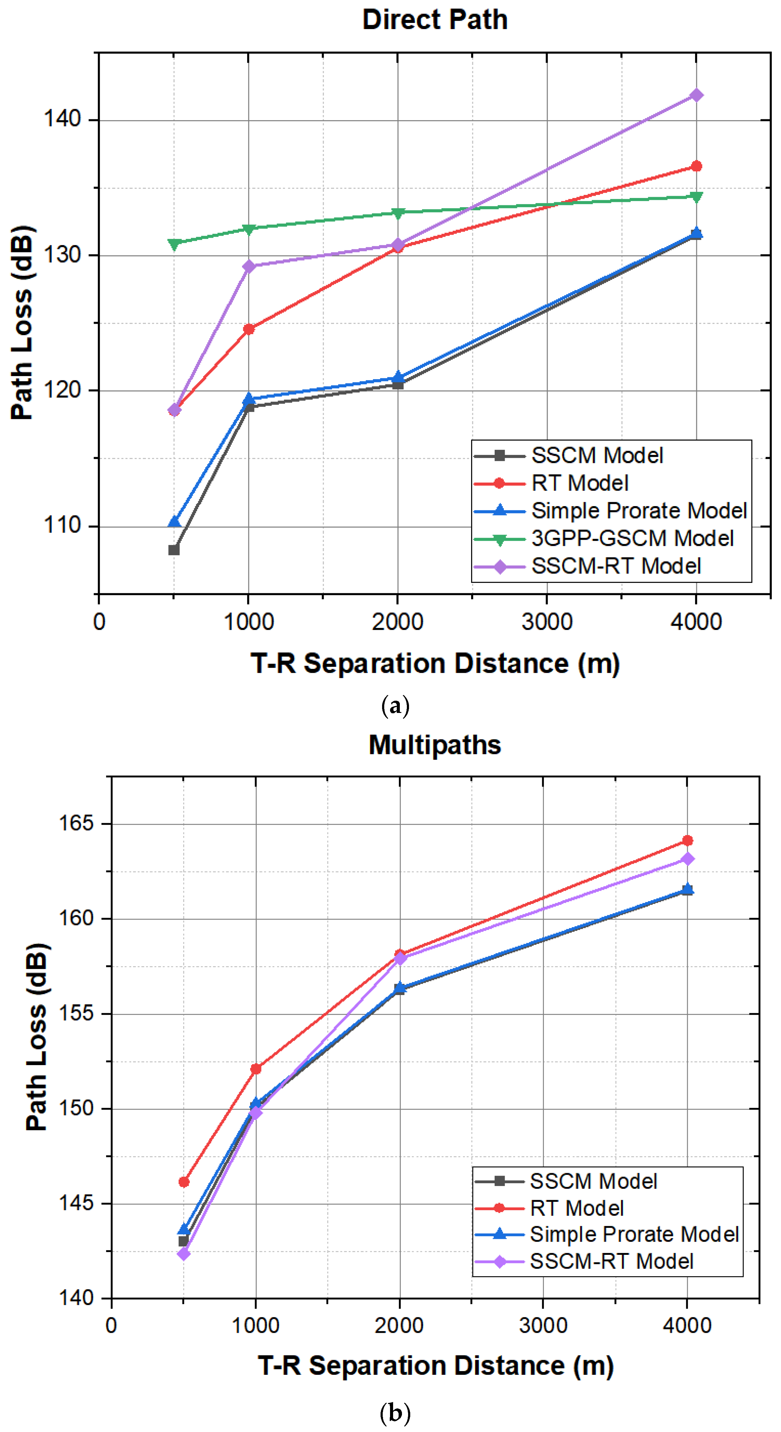
| SSCM Model | Direct Path | 108.22 dB | 118.82 dB | 120.49 dB | 131.51 dB |
| Multipaths | 143.00 dB | 150.09 dB | 156.27 dB | 161.49 dB | |
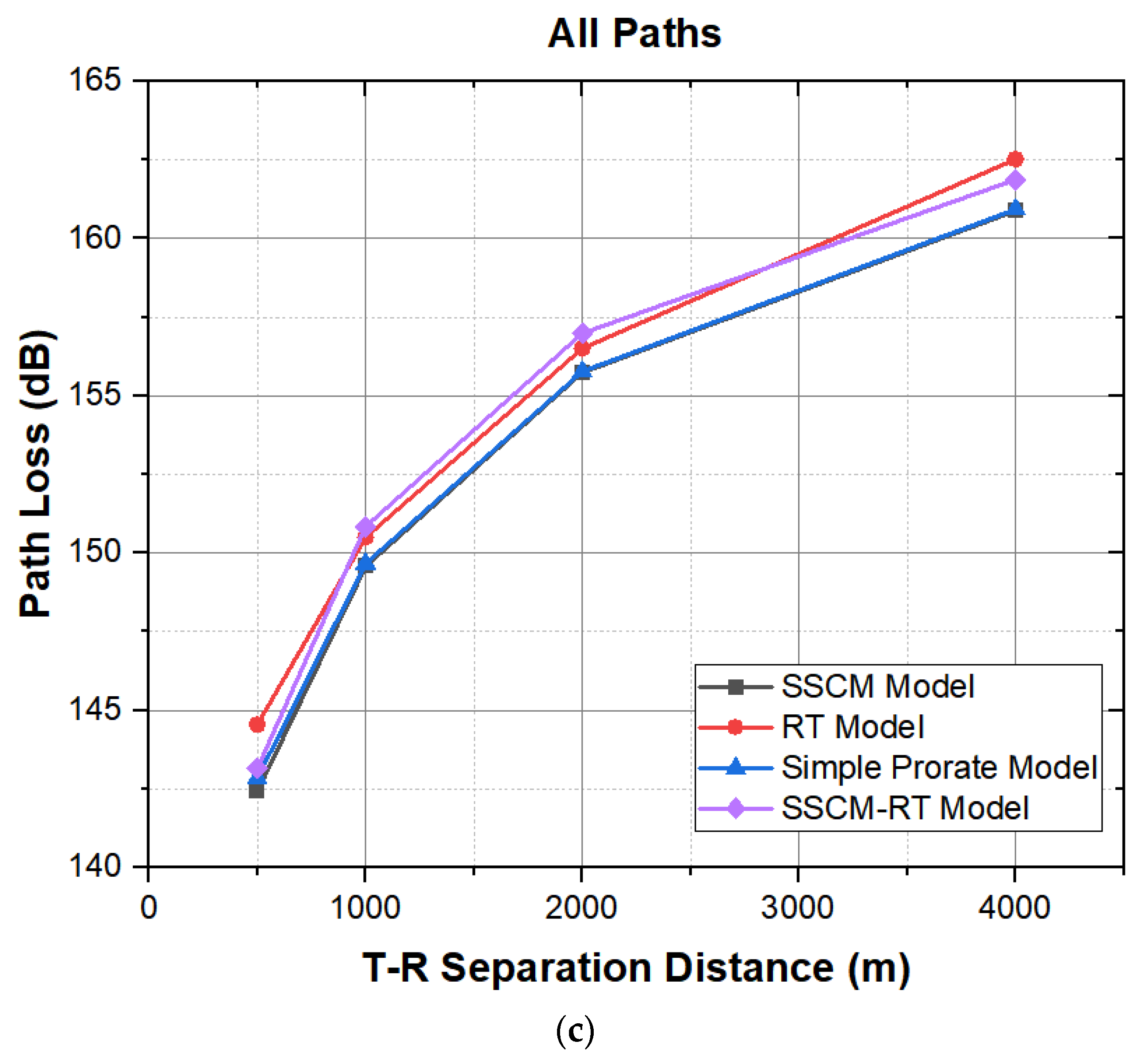
| All Paths | 142.42 dB | 149.57 dB | 155.73 dB | 160.88 dB | |
| RT Model | Direct Path | 118.55 dB | 124.57 dB | 130.59 dB | 136.61 dB |
| Multipaths | 146.17 dB | 152.12 dB | 158.12 dB | 164.14 dB | |
| All Paths | 144.54 dB | 150.50 dB | 156.50 dB | 162.52 dB | |
| Simple Prorate Model | Direct Path | 110.29 dB | 119.40 dB | 121.00 dB | 131.63 dB |
| Multipaths | 143.64 dB | 150.29 dB | 156.37 dB | 161.56 dB | |
| All Paths | 142.84 dB | 149.67 dB | 155.77 dB | 160.93 dB | |
| 3GPP-GSCM Model | Direct Path | 130.91 dB | 132.00 dB | 133.19 dB | 134.38 dB |
| SSCM-RT Model | Direct Path | 118.61 dB | 129.21 dB | 130.84 dB | 141.89 dB |
| Multipaths | 142.38 dB | 149.80 dB | 157.91 dB | 163.17 dB | |
| All Paths | 143.15 dB | 150.84 dB | 156.98 dB | 161.87 dB |
Disclaimer/Publisher’s Note: The statements, opinions and data contained in all publications are solely those of the individual author(s) and contributor(s) and not of MDPI and/or the editor(s). MDPI and/or the editor(s) disclaim responsibility for any injury to people or property resulting from any ideas, methods, instructions or products referred to in the content. |
© 2023 by the authors. Licensee MDPI, Basel, Switzerland. This article is an open access article distributed under the terms and conditions of the Creative Commons Attribution (CC BY) license (https://creativecommons.org/licenses/by/4.0/).
Share and Cite
Yang, J.; Xi, H.; Pan, Z.; Zhou, Y. UAV Dynamic Non-Terrestrial Transmission Channel Analysis Based on SSCM-RT Model. Symmetry 2023, 15, 1955. https://doi.org/10.3390/sym15101955
Yang J, Xi H, Pan Z, Zhou Y. UAV Dynamic Non-Terrestrial Transmission Channel Analysis Based on SSCM-RT Model. Symmetry. 2023; 15(10):1955. https://doi.org/10.3390/sym15101955
Chicago/Turabian StyleYang, Jinsheng, Huan Xi, Zhou Pan, and Ying Zhou. 2023. "UAV Dynamic Non-Terrestrial Transmission Channel Analysis Based on SSCM-RT Model" Symmetry 15, no. 10: 1955. https://doi.org/10.3390/sym15101955
APA StyleYang, J., Xi, H., Pan, Z., & Zhou, Y. (2023). UAV Dynamic Non-Terrestrial Transmission Channel Analysis Based on SSCM-RT Model. Symmetry, 15(10), 1955. https://doi.org/10.3390/sym15101955