Abstract
A deterministic model for the transmission dynamics of SIRS-type malaria in hosts and SI in mosquito populations is proposed. The host population is differentiated between naive, primary, and secondary susceptible individuals. Primary and secondary infected individuals (and also recovered) are differentiated from each other according to their degree of infectiousness. The impact of changing the relative susceptibilities of primary and secondary (with respect to naive) susceptible individuals on the dynamics is investigated. Also, the impact of changing the relative infectiousness of secondary infected, primary, and secondary recovered individuals (with respect to primary infected) on the transmission dynamics of malaria is studied.
1. Introduction
Malaria, a mosquito-borne infectious disease caused by the protozoan parasites of the genus Plasmodium, is transmitted to humans via bites from infected female Anopheles mosquitoes, which introduce the organisms from its saliva into the host’s circulatory system, which is potentially fatal. In humans, malaria is caused by Plasmodium falciparum, Plasmodium malariae, Plasmodium ovale, and Plasmodium vivax, with deaths caused primarily by P. falciparum and P. vivax, while P. ovale and P. malariae are typically responsible for milder forms of malaria. Malaria is prevalent around the equator, in tropical and subtropical regions that include much of Sub-Saharan Africa, Asia, and the Americas. The prevalence of malaria is tied in to circumstances connected to rainfall and temperature patterns, altitude, and the availability of appropriate larvae breeding sites (stagnant waters).
Malaria, an ancient disease [1,2], has instigated sustained efforts aimed at ameliorating its impact on populations using what has been learned from scientific research and epidemiological studies, which are frequently complemented with the results of analyses and simulations of mathematical models over the past few decades [3,4,5,6].
Malaria mathematical modeling at the population level essentially started with the work of Sir Ronald Ross [7] and was expanded and applied by Macdonald [8] and many others, including Dietz [9], Aron and May [10], Torress-Sorando and Rodriguez [11], Koella and Anita [12], and Filipe et al. [13]. Sir Ronald Ross shared the 1902 Nobel award in malaria through research that connected the life-cycle of the malaria parasite in hosts and vectors [14]. His 1911 paper introducing a nonlinear system of differential equations to study the transmission dynamics of malaria was groundbreaking and arguably the paper that established the field that is now known as mathematical epidemiology, which is tightly connected to the study of host–parasite dynamics, disease evolution, and vector control [7]. Macdonald extended Ross’s model by adding biological realism, with the aim of connecting questions to models and models to data [8,15,16,17,18]. In an early attempt to study the theory of eradication of malaria, Macdonald and his collaborators [17] analyzed the factors affecting the basic reproduction number, . Moreover, they discussed the epidemiology of malaria [18], with special reference to the pattern observed in equatorial Africa. In [16], Macdonald and Goeckel studied the effect of considering a complete interruption of transmission on the regular progressive decrease in the falciparum parasite over a specific period of time. Macdonald and Goeckel also estimated the slowest acceptable vivax fall-off rate over a 12-month period [16].
Certainly, the research that connected the life cycle of vectors, hosts, and parasites naturally brought exceeding interest to the study of the role of the immune system within hosts and across vectors and human malaria interactions. How would such interactions within and between individuals influence the levels of infectiousness, susceptibility, or re-infection after recovery? The challenges raised in connecting multiple levels of malaria dynamics and infections were probably addressed first by Dietz et al. [9], when these researchers incorporated the role of immunity at the population level. The use of malaria models to study specific questions exploded after the seminal work of Sir Ronald Ross and the innovative extensions carried out by Macdonald [15,16,17,18] and Dietz and his collaborators [9] (see also [19,20,21,22] and the references therein). Some reviews of the mathematical modeling and analysis of malaria are shown in [3,4,10,23,24,25]. Recent population-level efforts have included the role of genetics, with specific research carried out on the role of sickle cell anemia and the presence of large populations of asymptomatics [26,27]. More studies on the impact of climatic change and weather on malaria dynamics are shown in [20,28,29].
Ngwa and Shu [22] considered an SEIRS model for the host and SEI for the vector under the assumption that the population is closed and of varying sizes. It was assumed that recovered individuals are partially immune and yet still capable of transmitting the infection. They derived conditions for the existence of endemic equilibria and studied the global stability of the malaria-free equilibrium for , where is their basic reproduction number.
Chitnis et al. [30] considered an SEIRS model for the host and an SEI model for the vector. The authors considered an open population with recruitment through births and immigrating (susceptible) individuals. Their model supports the existence of an infection-free equilibrium that is locally asymptotically stable whenever . In their paper, it was shown that more than one endemic equilibrium may exist if . In a special case, where the malaria-induced mortality rate vanishes, the bifurcation at is forward.
Niger and Gumel [31] considered a model for malaria transmission dynamics with repeated exposure. The model has been analyzed and shown to exhibit the existence of multiple endemic equilibria when for certain parameter values, in case of standard incidence. However, the authors showed that if the repeated exposure is ignored and if the incidence function is of a mass-action type, the model is reduced to a simple SIRS model in the host and SI in the vector. The reduced model is shown to not have multiple endemic equilibria.
This paper uses mathematical models to expand on the role of the human immune system’s variability in the transmission dynamics of malaria and control. Specifically, we focus on the interplay between differences in susceptibility, ability by humans to increase or reduce the ’health’ of the parasite population, and differential levels of infectiousness; that is, the ability of humans to harbor effectively limited or large populations of parasites. The incorporation of heterogenous and variable levels of infectiousness and susceptibility bring unexpected, possibly unwanted, consequences to the forefront. Models that consider variation in susceptibility and infectiousness will invariably support multiple endemic states; that is, they naturally support disease dynamics that depend on initial conditions and that cannot be characterized by the basic reproduction number, a dimensionless quantity that has brought simplicity and clarity to those interested in finding ways of characterizing effectively simple and direct modes of malaria elimination or prevalence reductions. The fact is that variation in host susceptibility and infectiousness, the norm in biology, limits the preponderant role given to the basic reproduction number; the result of the theoretical work carried out by models that omit variation (a most important pre-requisite for selection).
More specifically, we developed a mathematical model where we differentiate between individuals who have never experienced the infection (called naive), those who experienced it only once (called primary), and those who experienced it at least twice (called secondary). The aim of this paper is to study the impact of changing the relative susceptibility and infectiousness of primary and secondary individuals on the disease dynamics in the human population.
The paper is organized as follows. In Section 2, we formulate the model and study the existence and stability of the malaria-free equilibrium. We further compute the basic reproduction number and find an equation that defines the endemic equilibrium human force of infection . In Section 3, we study the direction of bifurcation at and investigate the possible bifurcation diagrams in the plane . In Section 4, we study the impact of changing the relative susceptibilities and infectiousness in the population dynamics of the host and parasites. In Section 5, we study the role of differential mortality. We end the paper with a summary and conclusion in Section 6.
2. Model Formulation
2.1. Null Model
In this section, we introduce a null model, which allows us to state basic malaria model results in the absence of variation in infectiousness and susceptibility. It is an SIRS model for human populations and an SI model for mosquito populations. Here, the total human population (with size ) is subdivided into susceptible, infected, and recovered, whose size at time t is given by , and , respectively. The mosquito population (of size ) is subdivided into susceptible and infected , see Table 1 for more detailed description of the physical meaning. Both populations of interaction are assumed to be homogeneously and symmetrically fully mixed. The dynamics of interaction between both (human and mosquito) populations is governed by the model
where and are as defined in Table Table 2. The per-capita rate denotes the transition from to state, while the transition from to state is denoted by the per-capita rate . The malaria-induced mortality rate (in humans) is denoted by . Recovered individuals are assumed to be weakly infectious. Here, q denotes the infectiousness reductions for R- with respect to S-individuals. Equation (1) is defined on the closed set , where

Table 1.
Description of the state variables of Equation (5).
Table 2.
Description of the model parameters and their dimensions.
In the simple case, where deaths due to malaria are neglected (i.e., ), Equation (1) supports a malaria-free equilibrium that is stable if and only if the basic reproduction number for Equation (1) is less than one. Moreover, Equation (1) has a unique endemic equilibrium that exists only if the basic reproduction number is bigger than one; an equilibrium that is stable whenever it exists. On the other hand, whenever human deaths due to malaria are considered, we see that Equation (1) exhibits backward bifurcation for certain parameter values. The derivation of these results is deferred to Appendix A.
If we extend the above model by further subdividing the epidemiological classes and into naive susceptible representing those who have never experienced the infection, primary susceptible representing those who experienced it only once, and secondary susceptible to denote those who experienced malaria at least twice, then the dynamics supported by the model are enriched; an expected outcome when individuals are differentiated from each other by their susceptibilities. Similarly, infected humans are subdivided into primary infected, those who experience malaria for the first time, and secondary infected, those who are infected at least for the second time, with individuals in both classes supporting different degrees of infectiousness. Also, individuals in the class of recovered are categorized into primary recovered and secondary recovered. The extended model is shown in the next section. The aim of this paper is to study the impact of variation in susceptibility and infectiousness on the dynamics of malaria. (1) Do these extensions affect endemic behavior? (2) What is the impact of changing the relative susceptibilities of primary and secondary (with respect to naive) susceptible individuals on the dynamics and, therefore, on the elimination effort? (3) What is the impact of changing the relative infectiousness of secondary (with respect to primary) infected individuals? (4) What makes it possible to support multiple endemic equilibria?
2.2. Extended Model
To study the impact of differential susceptibility, infectiousness, and mortality on the dynamics of malaria (at the population level), we consider a model of type SIRS for humans and SI for mosquitoes. In such a model, individuals are epidemiologically asymmetric, but they are symmetric in their mixing behavior in the sense that they mix homogeneously so that each mosquito bite has an equal chance of transmitting the virus to susceptible humans in the population. The total host (human) population at time t, whose size is denoted by , is subdivided into seven mutually exclusive sub-populations: naive susceptible , primary infected , primary recovered , primary susceptible after experiencing the infection once before , secondary infected , secondary recovered , and secondary susceptible , so that . Naive susceptible human individuals are those who never experienced a malaria infection, while primary infected human individuals are hosts who acquired a malaria infection for the first time and are capable of transmitting malaria to susceptible mosquitoes while the mosquitoes are taking their meals from human individuals. Primary (secondary) recovered human individuals are human hosts who experienced malaria infection only once (at least twice) and became immunized, but are still slightly infectious [32]. Primary (secondary) susceptible individuals are susceptible human hosts who experienced malaria only once (at least twice) and recovered with partial immunity, in the sense that they are less susceptible to acquire malaria than naive susceptible ones. Secondary infected individuals are human individuals who acquired a malaria infection at least twice and are capable of transmitting it to susceptible mosquitoes, with differential transmissibility of the infection as opposed to primary infected ones. Table 1 shows briefly the physical meaning of the model state variables.
Similarly, the total vector (mosquitoes) population at time t, whose size is denoted by , is split into two sub-populations: susceptible mosquitoes and infectious mosquitoes , so that .
It is supposed that new recruits of the host enter the naive susceptible human sub-population class with recruitment rate and that deaths occur at the natural death per-capita rate in all human sub-population classes except those, for primary and secondary infected sub-populations, where excess deaths due to malaria are included. The malaria-induced mortality for primary and secondary infected individuals occurs at rates and , respectively. Naive susceptible humans either die of natural death () or acquire a malaria infection with force of infection , to become primary infected individuals who either die or recover to be primary recovered individuals with rate . Therefore, that rate of change in the number of naive susceptible and primary infected humans is described by two ordinary differential equations
Human individuals are supposed to stay primary recovered for a period of time before losing their acquired immunity to become primary susceptible, and then die naturally or become infected with rate to be secondary infected, where is the relative susceptibility of primary with respect to naive susceptible individuals. Therefore, we have the following subsystem of equations
It is worth explaining that the parameter () is a rescaling dimensionless parameter that accounts for the reduction in the susceptibility of individuals due to enhancing their immunity after experiencing a malaria infection only once (at least twice).
Secondary infected individuals either die or recover with rate to become secondary recovered, who are supposed to either die naturally or lose their immunity to become secondary susceptible. The rate at which secondary recovered individuals lose their immunity is . Finally, secondary susceptible individuals either die or become infected again with force of infection , where is the relative susceptibility of compartment individuals with respect to naive susceptible individuals. Therefore, we have the following sub-dynamical system
On the other hand, susceptible mosquito populations recruit with rate and either die naturally with rate , or become infected with force of infection , while infected mosquitoes are assumed to die naturally with the same rate . A schematic flow diagram for the model states is depicted in Figure 1, while a full description for the model variable states and parameters is given in Table 1 and Table 2, respectively. Following the same approaches shown in [31,33], the incidence rates and are given by
where the dimensionless parameters and account for the reduction in the infectiousness of human hosts who, respectively, acquired a malaria infection at least twice, recovered primarily from their malaria infection (and are assumed to be asymptomatic carriers), and recovered after experiencing the infection at least twice (assumed to be an asymptomatic carrier too), in comparison to individuals who were infected only once.
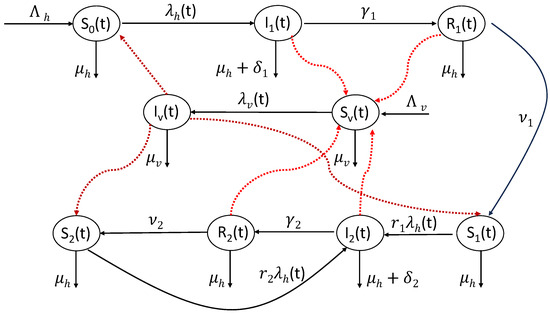
Figure 1.
A schematic diagram for the interaction and transition between the various states of Equation (5).
Collecting the above formulated equations together, we arrive at the following mathematical model of ordinary differential equations
where and are given by Equations (3) and (4), respectively. Moreover, all parameters are assumed to be strictly positive, with the exception of the parameters and , representing the malaria-induced human mortality rates, which are assumed to be nonnegative.
2.3. Existence and Stability of the Infection-Free Equilibrium and the Basic Reproduction Number
To find the equilibria, we put the derivatives in the left-hand side in Equation (5) equal to zero. The malaria-free equilibrium (MFE) is obtained by setting and solving the resulting system. Therefore, the MFE is
where denotes vector transpose.
2.3.1. The Basic Reproduction Number
The basic reproduction number is obtained using the next generation operator method [34]. Accordingly, we evaluate the matrices (for the new infection terms) and (for the transition terms) as
where
- is the time duration spent in the state;
- is the duration of time spent in the state;
- is the duration of time spent in the state;
- is the duration of time spent in the state;
- .
It follows then that the basic reproduction number is given by
where is the spectral radius (dominant eigenvalue in magnitude) of the matrix . It is clear that the basic reproduction number depends on the relative infectiousness of secondary infected (with respect to primary infected) individuals and depends neither on the relative susceptibilities nor on the relative infectiousness of recovered individuals.
2.3.2. Stability of the Malaria-Free Equilibrium:
To establish the stability of the malaria-free equilibrium, we linearize the model around it to obtain the Jacobian matrix (evaluated at the infection-free equilibrium) as
Using the columns number one, four, seven, and eight, one may compute four eigenvalues , , , for the Jacobian matrix . Then, we use row number five to obtain an eigenvalue of . Thereafter, we use row number six to obtain an eigenvalue of . All these six eigenvalues are negative. Thus, the remaining eigenvalues of are those of the sub-matrix
Hence, the stability of the Malaria-free equilibrium is determined by studying the roots of the characteristic equation of that is given by
where is the eigenvalue of . On simplifying and collecting terms together, we arrive at a cubic equation in the form
where
To this end, we apply the Routh–Hurwitz criterion [35]. We notice that and . Assume now that . Then, , which implies that
Thus, with the use of Equation (9), we deduce that and , for . We further notice that , , , and . However,
Hence, with the use of Equation (9), we deduce that both and are positive. Hence, based on the Routh–Hurwitz criterion [35], all roots of Equation (8) have a negative real part for .
We end this subsection by stating the following proposition on the local stability of the malaria-free equilibrium.
Proposition 1.
The malaria-free equilibrium is locally stable if and only if , while it is unstable otherwise.
2.4. Endemic Equilibria
Persistent solutions (endemic equilibria) are solutions where the infection is assumed to persist, in the sense that the prevalence of infection at equilibrium is positive. So, let us assume that the equilibrium human and vector force of infections and . Hence, on setting the derivatives in the left hand side of Equation (5) equal zero and solving the resulting system with respect to the state variables, one can obtain at equilibrium
and
Now, we use Equation (20) into Equation (4) to get
where, with the use of Equations (11), (12), (14), and (15)
On simplifying Equation (23), we get a nonlinear algebraic polynomial equation of degree six in the endemic host’s force of infection . Its term-free of is
while the coefficients of the other six terms with have very complicated mathematical expressions.
3. Bifurcation Analysis
3.1. Center Manifold Analysis near the Malaria-Free Equilibrium
The model we study has an endemic equilibrium equation with a polynomial of degree six in the endemic force of infection . This polynomial has six solutions. However, of interest are only feasible solutions, in the sense that these solutions are real and positive. Also, it is more interesting if these feasible solutions exist for values of .
On setting in the equilibrium Equation (23), we get , where
This value corresponds to . Thus, in the plane , there is a bifurcation point given by , at which we compute the direction of bifurcation. Using the theorem 4.1 of Castillo-Chavez and Song [36], the conditions ensuring the existence of backward bifurcation have been derived and are shown in Appendix B. The computations show that Equation (5) undergoes backward bifurcation at if and only if , where
On performing a sensitivity analysis of the expression K with respect to the parameters , and , we find that and are the most sensitive parameters. Namely speaking, is more sensitive than , which in turn is more sensitive than . Therefore, the inequality required for the existence of backward bifurcation is expressed as
Figure 2 shows the area in the planes and for which the bifurcation is subcritical (backward) as well as that in which it is supercritical (forward). It shows that the possibility for the existence of backward bifurcation increases with the increase in , while it decreases as increases. Based on the above analysis, we summarize our results in the following proposition.
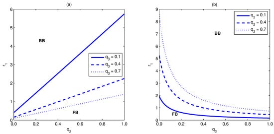
Figure 2.
The area for backward as well as forward bifurcation. Part (a) shows these regions in the plane for several values of . It shows that the backward bifurcation region extends with the increase in the value. However, part (b) shows that, in the plane , the backward bifurcation region shrinks with the increase in the value. Simulations have been done for the parameter values given in Table 3.
3.2. Possible Bifurcation Diagrams
Equation (23) could be seen as a function in the contact rate . Since the expressions , and do not depend on , we can rewrite Equation (23) in terms of as
where
It is easy to check that . Therefore, and . Since , then . Thus, all coefficients and are positive. Hence, Equation (27) has the unique positive solution
Assume now that the equilibrium human force of infection is known. In order to study the possible bifurcation diagrams, we investigate the number of feasible turning points. By a feasible turning point we mean a turning point that occurs at a positive value of the force of infection . To do so, we study and count the number of possibly feasible solutions of the equation
If Equation (29) has no feasible solution, then the model shows only forward bifurcation, Figure 3a. However, if it has a unique feasible solution, then it shows a backward bifurcation, Figure 3d. If it has two feasible solutions, then the model shows the existence of hysteresis, in the sense that it shows multiple super- and subcritical endemic states where the bifurcation curve looks like those shown in Figure 3b,c.
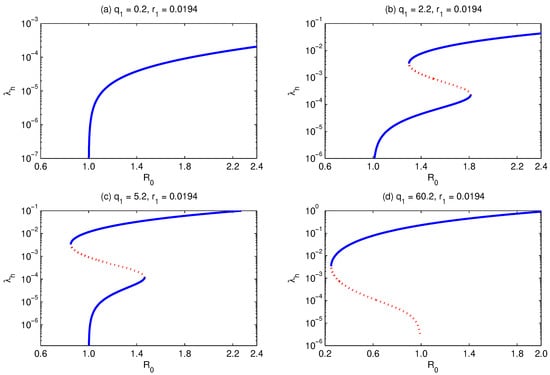
Figure 3.
Bifurcation diagram for . It shows that with the increase in , while fixing and all other parameters, the model develops forward (a), multiple supercritical (b), multiple subcritical (c), and backward (d) bifurcations. Simulations have been done for the parameter values given in Table 3, except for and as stated above.
Since the functions are polynomials of degree 3, while is a polynomial of degree 2 in the variable , then according to formula (28) the expression under the square root in (28) would be a polynomial of degree 8. Moreover, this expression is added and multiplied with other polynomials and the whole thing is divided by some other polynomials. All of these, along with the Equation (29), lead to a complicated nonlinear algebraic (with square root function) equation from which we compute the turning points. It is difficult, if not impossible, to find exact formulae for the turning points and also for the constraints on model parameters which assure the existence of such feasible points. Therefore, numerical simulations have been performed.
For our model, extensive simulations have been made and we found out that the model may show forward, multiple supercritical, multiple subcritical, and backward bifurcations, as we shall see in the next section, where we study the impact of the relative susceptibilities , relative infectiousness , and the differential mortalities and on developing all these kinds of bifurcations.
4. Role of Differential Susceptibility and Infectiousness
Differential susceptibility and differential transmissibility/infectiousness play a key role not only in the type of bifurcation but also in the shape of the bifurcation curve. In the following we try to, numerically, figure out the role of changing the relative susceptibilities as well as the relative infectiousness and in the overall bifurcation dynamical behavior. This is assessed by letting the parameter of interest have changing values (in various ways) while fixing the remaining model parameters and noticing the type of the resulting bifurcation diagram. It is worth mentioning that the bifurcation diagram gives information on the number of endemic equilibria and the minimum value of the basic reproduction number under which the malaria infection dies out. In other words, it gives information about the minimum elimination effort required to eliminate the malaria infection [39]. We first consider the case that recovered individuals are not capable of transmitting malaria which, mathematically, means that .
4.1. Non-Infectious Recovered Individuals
In this case, the basic reproduction number reduces to
while the condition (26), on the relative susceptibility of individuals in compartment , with respect to naive susceptible individuals, for backward bifurcation reduces to
Relation (31) shows that the critical level for backward bifurcation does not depend on the relative susceptibility (of secondary with respect to naive susceptible human individuals) , but depends on the relative infectiousness (of secondary with respect to primary infected human individuals) and other model parameters. Thus, for fixed , the backward bifurcation condition (31) is a decreasing function in , see Figure 4, while for fixed , it is constant. On the other hand, Equation (23), from which we determine the equilibrium human force of infection, remains at degree six. Numerical simulations have been made to detect the progression of the shape of the bifurcation curve with the increase in one of the relative susceptibilities and the relative infectiousness while fixing the other two parameters, with the remaining model parameter values as shown in Table 3.
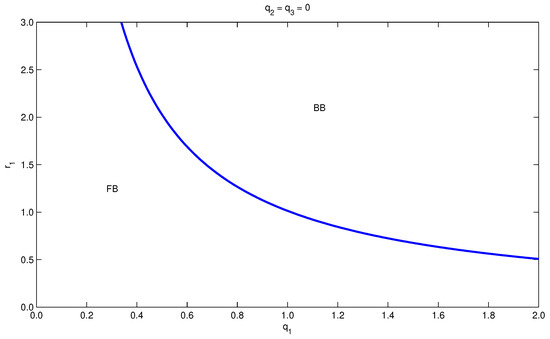
Figure 4.
Bifurcation diagram in the plane , for and with parameter values as in Table 3. High enough values of and exhibits the existence of backward bifurcation.
Table 3.
Table showing numerical values of parameters used in the numerical manipulations and the references (when applicable).
4.1.1. Impact of the Relative Infectivity Ratio
In order to assess the impact of changing the relative infectiousness of secondary (with respect to primary) infected individuals on the model dynamics during a long-time run, we let change and fix the other model parameters. In this case, the resulting bifurcation diagram looks like that shown in Figure 3 and Figure 5. For fixed high-enough values of the relative susceptibility of primary susceptible with respect to naive susceptible human individuals , while increasing , the bifurcation curve progresses from the case where there is exactly one supercritical endemic equilibrium, Figure 5a, to the case where there are two subcritical endemic equilibria but only one supercritical endemic equilibrium (i.e., backward bifurcation), Figure 5b. However, if we choose to be small enough (e.g., ) and letting increase (Figure 3), the shape of the bifurcation curve changes from a simple forward bifurcation (Figure 3a) to a backward bifurcation (Figure 3d), passing through the formulation of hysteresis (Figure 3b,c).
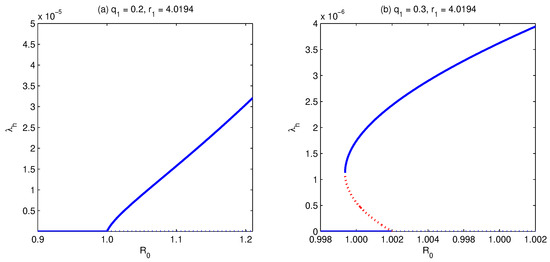
Figure 5.
Bifurcation diagram for . It shows that with the increase in , while fixing , and all other parameters, the model develops forward (a) to backward (b) bifurcation. Simulations have been done for the parameter values given in Table 3, except for and as stated above.
4.1.2. Impact of the Relative Susceptibility Ratio
On the other hand, if we fix the relative infectiousness ratio (of secondary infected relative to primary infected human individuals) and let the relative susceptibility ratio increase, the model shows the following two behaviors concerning the bifurcation curve. The first is that for a fixed value of in a certain range (e.g., ), if we let be small enough (), the bifurcation curve represents the situation where there is exactly one supercritical endemic equilibrium (i.e., simple forward bifurcation), Figure 6a. However, if we let increase (), then the model exhibits the existence of multiple supercritical endemic equilibria, Figure 6b. If we further let increase (), the model shows again the existence of a unique supercritical endemic equilibrium, Figure 6c. Also, if we let be bigger than (), then a backward bifurcation appears, Figure 6d.
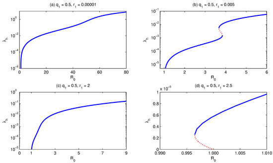
Figure 6.
Bifurcation diagram for . It shows that for small , while fixing and all other parameters, but increasing , the model develops forward (a–c) to backward (d) bifurcation. Simulations have been done for the parameter values given in Table 3, except for and as stated above.
Unlike the above case, if we choose the relative infectiousness to be large, then, with the increase in the relative susceptibility , the bifurcation curve develops from forward bifurcation (Figure 7a) to forward with multiple supercritical endemic equilibria (Figure 7b), forward with multiple subcritical endemic equilibria (Figure 7c), and then backward bifurcation (Figure 7d).
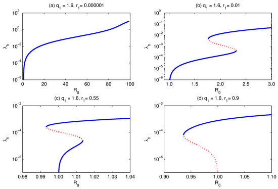
Figure 7.
Bifurcation diagram for . It shows that for and keeping and all other parameters fixed, except , which is allowed to increase, the model develops forward (a), multiple supercritical (b), multiple subcritical (c), and backward (d) bifurcation. Simulations have been done for the parameter values given in Table 3, except for and as stated above.
4.1.3. Impact of the Relative Susceptibility
On fixing the relative infectiousness (of secondary infected with respect to primary infected human individuals) , the condition (31) for backward bifurcation says that the critical level of the relative susceptibility (of primary with respect to naive susceptible human hosts) is constant. Thus, for any fixed value of the relative infectiousness (e.g., ), then the critical value of the relative susceptibility above which the bifurcation is backward would be constant (). Here, we have three situations.
- The first one is to consider to be small enough (e.g., ). Here, if we let increase, then the bifurcation curve would progress as follows. For small values of (e.g., ), the bifurcation diagram shows the existence of exactly one supercritical endemic equilibrium (similar to that shown in Figure 6a). If we increase (e.g., ), then we get a bifurcation curve for which a forward bifurcation as well as multiple supercritical endemic equilibria are exhibited (similar to that shown in Figure 6b). However, on letting increase further, the bifurcation curve becomes forward with a unique endemic equilibrium, similar to that shown in Figure 6c. Thus, in this case, multiple subcritical and supercritical endemic equilibria are impossible to exist.
- The second situation is to consider slightly larger values of (e.g., ), but still less than . In this case, for small values of the relative susceptibility (of secondary with respect to naive susceptible human individuals) (e.g., ), the model shows the existence of a unique endemic equilibrium, Figure 8a. However, for larger values of (), the model exhibits forward as well as multiple supercritical endemic equilibria, but no subcritical endemic equilibria, Figure 8b. If is increased further (), the model shows the existence of forward bifurcation as well as sub- and supercritical endemic equilibria, Figure 8c. If is assumed to further increase, then the critical value of (at the turning point) separating between nonexistence and existence of endemic equilibria decreases (Figure 8d), which implies an increase in the effort required to eliminate the malaria infection [39].
- The last situation is to consider values of the relative susceptibility (of primary with respect to naive susceptible human hosts) (e.g., ). In this case, the model exhibits backward bifurcation, but what is important is that increasing the value of the relative susceptibility (of secondary with repect to naive susceptible human hosts) implies a decrease in the value of the critical separating between the nonexistence and existence of endemic equilibria, which in turn increases the minimum effort required to eliminate malaria, Figure 8e–h.
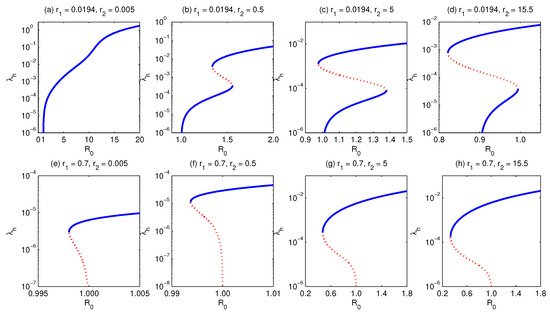
Figure 8.
Bifurcation diagram for and for fixed . It shows that for a value of , increasing the relative susceptibility , while fixing all other parameters, the model develops forward (a), multiple supercritical (b), and multiple subcritical (c,d) bifurcation, but it cannot exhibit backward bifurcation. However, for , the model exhibits backward bifurcation where the critical value of at which the turning point occurs decreases, (e–h). This induces an increase in the elimination effort. Simulations have been done for the parameter values given in Table 3, except for and as stated above.
We summarize our results as the following: if the infectivity of recovered individuals is ignored (i.e., ), then,
- For small enough values of the relative infectiousness (i.e., for values of on the left of the dotted vertical line in Figure 9), the model undergoes backward bifurcation as the relative susceptibility increases.
- If the relative infectiousness of secondary infected individuals is allowed to be fairly increased (e.g., for values of between the two vertical lines in Figure 9), then (as increases) the progression of the bifurcation diagram is as follows: a forward bifurcation (with the existence of a unique endemic equilibrium for ) is exhibited. Then, a forward bifurcation with multiple supercritical endemic equilibria (hysteresis) is shown. Then, it exhibits again a forward bifurcation with unique endemic equilibrium for . Finally, it undergoes backward bifurcation.
- If is further increased (e.g., for values corresponding to higher than that at the vertical dashed line in Figure 9), then the model shows transcritical bifurcation for small values of , which is followed by forward bifurcation with multiple supercritical endemic equilibria as increases. If is further increased, then the model shows the existence of forward with multiple super and subcritical endemic states (hysteresis) and finally, it undergoes backward bifurcation.
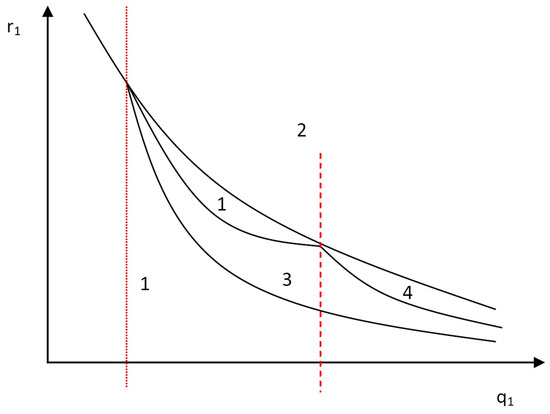
Figure 9.
A schematic bifurcation diagram for the case in the plane . The notation: 1 means a forward bifurcation with unique endemic equilibrium for ; 2 means backward bifurcation; 3 means forward bifurcation with multiple supercritical endemic states only (i.e., multiple equilibria exist only for , but no endemic equilibrium exists for ); 4 means forward bifurcation with multiple super- and subcritical endemic states (i.e., multiple equilibria exist for and for ).
The interpretation of the appearance of backward bifurcation and hysteresis phenomena is that in some season the mosquitoes are feeding and breeding and therefore their population size is growing. During such a season (like summer) they live long enough to cause malaria. This explains the sudden increase in infection levels. However, in other seasons where the female mosquitoes don’t live enough to cause malaria, we get a sudden decrease in the level of infection.
4.2. Infectious Recovered Individuals
Now, we assess the impact of changing the relative infectiousness parameters of primary and secondary recovered individuals on the endemic behavior of Equation (5). Therefore, we consider the general case where none of the model parameters are neglected. More precisely, we assume that recovered individuals are capable of transmitting the infection with relative infectiousness .
4.2.1. Impact of the Relative Infectiousness
To figure out the role of the relative infectiousness of secondary recovered individuals (with respect to primary infected human individuals) , we assume that as well as the other model parameters are constant, except , which is assumed to be increased, see Figure 10. The figure shows how the shape of the bifurcation curve can change as the value of increases. We notice that for small values of , the model exhibits forward bifurcation with a unique endemic equilibrium, Figure 10a. On increasing the value of , the model shows the existence of hysteresis, where there are two turning points, Figure 10b,c. In part (b) of the figure, there is a forward bifurcation with multiple supercritical, but not subcritical, endemic equilibria. However, with the increase in we, additionally, get multiple subcritical endemic equilibria, Figure 10c. If we allow to further increase, the model exhibits backward bifurcation, where there exist two subcritical endemic equilibria but only one supercritical endemic equilibrium, Figure 10d. It is clear that the increase in value implies a decrease in the critical basic reproduction level below which the infection does not persist, and therefore, it implies an increase in the minimum elimination effort of the malaria infection [39].
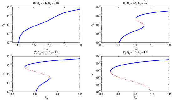
Figure 10.
Bifurcation diagram for . It shows that for , and keeping all other parameters fixed, except , which is allowed to increase, the model develops forward (a), multiple supercritical (b), multiple subcritical (c), and backward (d) bifurcation. Simulations have been done for the parameter values given in Table 3, except for and .
4.2.2. Impact of the Relative Infectiousness
Similar to above, if we assume the relative infectiousness (of primary recovered with respect to primary infected human individuals) changes, and we let all other parameters be fixed (see the legend of Figure 11 to get to know the parameter values), then the bifurcation curve progression has a different behavior compared with the case of . For small values of , the model shows the existence of backward bifurcation, Figure 11a. On letting increase, the model exhibits forward bifurcation with multiple supercritical with (and without) subcritical endemic equilibria. A further increase in values implies the existence of forward bifurcation, where no subcritical endemic equilibria exist but exactly one endemic equilibrium does exist. This implies that a reduction in values implies an increase in the minimum elimination effort of malaria.
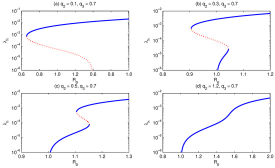
Figure 11.
Bifurcation diagram for . It shows that for , and keeping all other parameters fixed, except , which is allowed to increase, the model develops backward (a), multiple subcritical (b), multiple supercritical (c), and forward (d) bifurcation. Simulations have been performed for the parameter values given in Table 3, except for and .
5. Role of Differential Mortality
In this section, we figure out the dynamics of the model if the infection-induced mortality rates and are neglected. In this case, the equilibrium human population size is simply . Hence, and thus the left-hand size of Equation (23) would be reduced to a polynomial of degree three. If we further assume that recovered individuals are not capable of transmitting malaria, then the basic reproduction number reduces to
while the condition (26) for backward bifurcation reduces to
On the other hand, the Equation (23) from which we determine the equilibrium human force of infection reduces to
where and
and
It is clear that the coefficient , while the other three coefficients, namely and , can be positive or negative. Thus, Equation (34) could have up to three feasible solutions depending on the model parameter values, see Figure 12. This could be verified by studying the number of possible turning points in the bifurcation curve in the plane . To this end, Equation (34) is rearranged in a way such that the parameter (considered as a bifurcation parameter) is written as a function of the equilibrium force of infection , say . The number of feasible solutions for the equation determines the number of turning points. Thus, the equilibrium force of infection at a turning point satisfies the equation
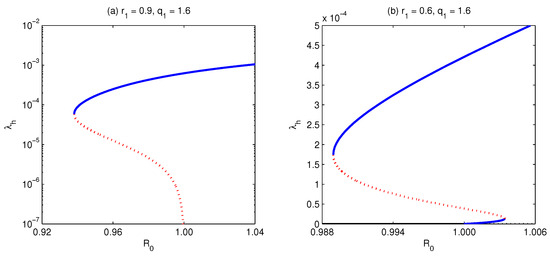
Figure 12.
Bifurcation diagram for . The figure is depicted for parameter values and keeping all other parameters fixed as in Table 3, except , which is allowed to take values and , as shown in the head of the sub-figures. The model develops backward bifurcation, (a). Moreover, it shows forward bifurcation with the existence of multiple supercritical and subcritical endemic equilibria, (b).
It is clear that the coefficients of the two terms and are non-negative, while the other coefficients can be positive or negative. Thus, the number of sign changes in the coefficients of Equation (35) determines the number of feasible solutions. On the other hand, it is easy to check that at , the bifurcation is backwards if and only if the term-free of in Equation (35) is negative. This means . Therefore, the coefficient of in Equation (35) is
If we assume the coefficient of in Equation (35) to be negative, then (irrespective of the sign of the -coefficient) the number of sign changes will be one, and therefore there is a unique feasible solution of Equation (35). However, if we assume that the -coefficient is positive, then, according to Equation (36), the -coefficient will be positive, and thus a unique solution for Equation (35) exists. Hence, if the bifurcation is backward, then there is a unique feasible turning point in the bifurcation curve drawn in the plane.
Similarly, the case of forward bifurcation is argued. In this case, the term-free of in Equation (35) is assumed to be positive. Thus, two feasible solutions for Equation (35) may exist if either or both coefficients of the and are negative, while otherwise there is no solution. We summarize our result in the following proposition.
Proposition 3.
If the malaria-induced mortality rates as well as the infectivity of recovered individuals are neglected, the model exhibits backward bifurcation if and only if the condition (33) holds. Moreover, it shows the existence of multiple sub- and supercritical (hysteresis) endemic equilibria, with two turning points at the most.
Simulations have been performed for this case and these show that the model can show backward bifurcation and hysteresis (the existence of supercritical and subcritical endemic states) phenomena.
6. Summary and Conclusions
A mathematical model for the transmission dynamics of malaria is proposed. The model is of type SI in the vector and SIRS in the host. For the host population, it is differentiated between individuals who have never experienced the infection (called naive), individuals who experienced the infection only once (called primary), and those who experienced it at least twice (called secondary). It is assumed that primary and secondary infected individuals have different infectiousness, where the relative infectivity of secondary (with respect to primary) infected individuals is . Also, the susceptibility of primary and secondary susceptible individuals is different from naive susceptible individuals (those who have never experienced the infection). The relative susceptibility of primary and secondary (with respect to naive) susceptible individuals are and , respectively. Moreover, it is assumed that recovered individuals have some immunity to malaria. They do not become clinically ill, but they do harbor low levels of parasites in their blood streams, and therefore they can pass the infection to mosquitoes. It is further assumed that the relative infectiousness of primary and secondary recovered (with respect to primary infected) individuals are and , respectively.
The analysis shows that the model has a malaria-free equilibrium, which is proven to be locally asymptotically stable for , while it is unstable if . Here, is the basic reproduction number and is given by Equation (7). Center manifold analysis shows that the model exhibits backward bifurcation if the expression in Equation (25) is positive. Local sensitivity analysis for this expression shows that the most sensitive parameters are and . Therefore, the backward bifurcation condition is expressed in the form of condition (26). This backward bifurcation condition (26) does depend on the parameters , and , but it does not depend on the relative susceptibility .
The equilibrium human force of infection is shown to be determined from the roots of a polynomial of degree six, which supports the possible existence of more than two endemic equilibria for certain model parameter values. However, in the special case and , the analytical results show that the bifurcation diagram in the plane () can have up to two turning points, which means that the model shows the existence of forward hysteresis (i.e., the existence of forward bifurcation with multiple super- and subcritical endemic steady states). On the other hand, in the general case, numerical simulations have been employed to investigate the impact of changing the relative susceptibilities , the relative infectiousness , and the differential mortalities on the development of the bifurcation diagram and therefore on the persistence of malaria.
The implication of the appearance of multiple super and subcritical endemic states is that the basic reproduction number is no longer an indicator in the malaria control process. This has an effect, especially on the value of the critical threshold value of , below which malaria infection does not persist, especially in the case of multiple subcritical endemic states. In this case, malaria does persist, even for values of . Consequently, the minimum effort required to control (eliminate) malaria is increased. Throughout the analysis, we came up with the following concluding remarks:
- The higher the value of either or both of the relative susceptibilities (of primary susceptible) and infectiousness (of secondary infected) is, the higher the effort needed to eliminate malaria is.
- The higher the value of the relative infectiousness of secondary recovered individuals is, the higher the effort required to eliminate malaria is.
- The higher the value of the relative infectiousness of primary recovered individuals is, the lower the effort required to eliminate malaria is.
It is worth mentioning that our model could be extended to include factors representing the control of malaria. Among the strategies that could be considered in a future extended model are the use of insecticide-treated bed nets by the human hosts and studying the optimization of who should use these treated bed nets.
Limitation of the Work and Probable Future Work
It is worth mentioning that our model neglects various factors that significantly affect malaria dynamical spread. Among these factors are environmental factors, like temperature, rainfall, and humidity. These factors impact mosquito and parasite vital rates, and thus affect the transmission intensity, seasonality, and geographical distribution of malaria. Also, the latency period of malaria has been neglected and may cause inaccurate estimations in the effort needed to control malaria. Other factors include biological and physiological differences between human males and females. Some or all of these factors will be considered in a forthcoming work.
Author Contributions
Conceptualization, M.S. and C.C.-C.; methodology, M.S.; software, M.S.; validation, M.S.; formal analysis, M.S. and A.A.; resources, M.S.; writing—original draft preparation, M.S., D.B., K.E.Y. and C.C.-C.; writing—review and editing, M.S. and A.A.; supervision, M.S. All authors have read and agreed to the published version of the manuscript.
Funding
This research received no external funding and The APC was funded by A.A.
Data Availability Statement
Not applicable.
Conflicts of Interest
The authors declare no conflict of interest.
Appendix A. Equilibrium Analysis of Model (1)
On putting the derivatives in the left hand side of Equation (1) equal zero and solving the resulting algebraic system in the state variables , we get
- The first scenario is . This implies that , and therefore, and . This is the malaria-free equilibrium for Equation (1).
- The second scenario is . In this case, the rearrangement of the terms results in the following quadratic equation in the equilibrium force of infectionwhereOnce we obtain a feasible solution of (A12), we substitute in (A4)–(A8) to obtain the corresponding equilibrium. At , we may derive the basic reproduction number for Equation (1) asIt is noteworthy that Equation (A12) is quadratic in and the number of feasible solutions could be determined by employing the implicit function theorem by following the approach shown in [40]. Moreover, the left hand side of Equation (A12) could be seen as a bifurcation equation in the equilibrium force of infection and the bifurcation parameter . Moreover, based on the use of the implicit function theorem, we may haveAt the bifurcation point in the plane we getwhereAlso,HenceThus, Equation (1) exhibits backward bifurcation if and only ifThe backward bifurcation condition (A15) implies that two malria-endemic equilibria do exist for values of . However, in the simple case , the condition (A15) does not hold and, consequently, the model has a unique malaria-endemic equilibrium if and only if .The stability analysis of the malaria-free equilibrium for Equation (1) could be established by following the same approach shown in Section 2.3. However, the stability analysis of the malaria endemic equilibrium of Equation (1) for values of could be established by following the same approach shown in [33].
Appendix B. Backward Bifurcation Conditions for Model (5)
To compute the direction of bifurcation for Equation (5) at , we make use of theorem 4.1 of Castillo-Chavez and Song [36]. It can be checked that the Jacobian evaluated at (i.e., ) has:
- a simple eigenvalue 0, while all other eigenvalues have negative real parts. Therefore, the center manifold theory can be used to analyze the dynamics of Equation (5),
- a left eigenvector and a right eigenvector , whereand
Thus, the assumptions of theorem 4.1 of Castillo-Chavez and Song [36] are held. Accordingly, the dynamics of the model near the malaria-free equilibrium is determined by the two quantities
where and is the right hand side of Equation (5). On performing some calculus, we get
As the expression is positive, then according to theorem 4.1 of Castillo-Chavez and Song [36], the Equation (5) undergoes backward bifurcation at if and only if the expression is positive. It is clear that the sign of depends mainly on the sign of the expression
Hence, if and only if .
References
- Cox, F.E. History of the discovery of the malaria parasites and their vectors. Parasites Vectors 2010, 3, 5. [Google Scholar] [CrossRef]
- Wirth, D. Malaria: A 21st century solution for an ancient disease. Nat. Med. 1998, 4, 1360–1362. [Google Scholar] [CrossRef] [PubMed]
- Koella, J.C. On the use of mathematical models of malaria transmission. Acta Trop. 1991, 49, 1–25. [Google Scholar] [CrossRef] [PubMed]
- Mandal, S.; Sarkar, R.R.; Sinha, S. Mathematical models of malaria —A review. Malar. J. 2011, 10, 202. [Google Scholar] [CrossRef] [PubMed]
- Tumwiine, J.; Mugisha, J.Y.T.; Luboobi, L.S. A mathematical model for the dynamics of malaria in a human host and mosquito vector with temporary immunity. Appl. Math. Comput. 2007, 189, 1953–1965. [Google Scholar] [CrossRef]
- Yang, H.M. Malaria transmission model for different levels of acquired immunity and temperature-dependent parameters (vector). Rev. Saude Publica 2000, 34, 223–231. [Google Scholar] [CrossRef]
- Ross, R. The Prevention of Malaria; John Murray: London, UK, 1911. [Google Scholar]
- Macdonald, G. The epidemiology and control of malaria. In The Epidemiology and Control of Malaria; CABI: Wallingford, UK, 1957. [Google Scholar]
- Dietz, K.; Molineaux, L.; Thomas, A. A malaria model tested in the African savannah. Bull. World Health Organ. 1974, 50, 347. [Google Scholar]
- Aron, J.L.; May, R.M. The population dynamics of malaria. In The Population Dynamics of Infectious Disease: Theory and Applications; Anderson, R.M., Ed.; Chapman and Hall: London, UK, 1982; pp. 139–179. [Google Scholar]
- Torres-Sorando, L.; Rodriguez, D.J. Models of spatio-temporal dynamics in malaria. Ecol. Model. 1997, 104, 231–240. [Google Scholar] [CrossRef]
- Koella, J.C.; Antia, R. Epidemiological models for the spread of anti-malarial resistance. Malar. J. 2003, 2, 3. [Google Scholar] [CrossRef]
- Filipe, J.A.N.; Riley, E.M.; Drakeley, C.J.; Sutherl, C.J.; Ghani, A.C. Determination of the processes driving the acquisition of immunity to malaria using a mathematical transmission model. PLoS Comput. Biol. 2007, 3, e255. [Google Scholar] [CrossRef]
- Ross, R. Inaugural lecture on the possibility of extirpating malaria from certain localities by a new method. Br. Med. J. 1899, 2, 1. [Google Scholar] [CrossRef] [PubMed]
- MacDonald, G.; Cuellar, C.B.; Foll, C.V. The dynamics of malaria. Bull. World Health Organ. 1968, 38, 743. [Google Scholar]
- Macdonald, G.; Göckel, G.W. The malaria parasite rate and interruption of transmission. Bull. World Health Organ. 1964, 31, 365. [Google Scholar] [PubMed]
- Macdonald, G. Theory of the eradication of malaria. Bull. World Health Organ. 1956, 15, 369. [Google Scholar] [PubMed]
- Macdonald, G. Epidemiological basis of malaria control. Bull. World Health Organ. 1956, 15, 613. [Google Scholar]
- Aron, J.L. Mathematical modeling of immunity to malaria. Math. Comput. Model. 1989, 12, 1180. [Google Scholar] [CrossRef]
- Gething, P.W.; Smith, D.L.; Patil, A.P.; Tatem, A.J.; Snow, R.W.; Hay, S.I. Climate change and the global malaria recession. Nature 2010, 465, 342–345. [Google Scholar] [CrossRef]
- Ngwa, G.A. On the population dynamics of the malaria vector. Bull. Math. Biol. 2006, 68, 2161–2189. [Google Scholar] [CrossRef]
- Ngwa, G.A.; Shu, W.S. A mathematical model for endemic malaria with variable human and mosquito populations. Math. Comput. Model. 2000, 32, 747–763. [Google Scholar] [CrossRef]
- Anderson, R.M.; May, R.M. Infectious Diseases of Humans: Dynamics and Control; Oxford University Press: Oxford, UK, 1991. [Google Scholar]
- Dietz, K. Mathematical models for transmission and control of malaria. In Malaria: Principles and Practice of Malariology; CABI: Wallingford, UK, 1988; Volume 2, pp. 1091–1133. [Google Scholar]
- Nedelman, J. Introductory review some new thoughts about some old malaria models. Math. Biosci. 1985, 73, 159–182. [Google Scholar] [CrossRef]
- Feng, Z.; Smith, D.L.; McKenzie, F.E.; Levin, S.A. Coupling ecology and evolution: Malaria and the S-gene across time scales. Math. Biosci. 2004, 189, 1–19. [Google Scholar] [CrossRef] [PubMed]
- Shim, E.; Feng, Z.; Castillo-Chavez, C. Differential impact of sickle cell trait on symptomatic and asymptomatic malaria. Math. Biosci. Eng. MBE 2012, 9, 877. [Google Scholar]
- Paaijmans, K.P.; Read, A.F.; Thomas, M.B. Understanding the link between malaria risk and climate. Proc. Natl. Acad. Sci. USA 2009, 106, 13844–13849. [Google Scholar] [CrossRef] [PubMed]
- Parham, P.E.; Michael, E. Modeling the effects of weather and climate change on malaria transmission. Environ. Health Perspect. 2010, 118, 620–626. [Google Scholar] [CrossRef] [PubMed]
- Chitnis, N.; Hyman, J.M.; Cushing, J.M. Determining important parameters in the spread of malaria through the sensitivity analysis of a mathematical model. Bull. Math. Biol. 2008, 70, 1272–1296. [Google Scholar] [CrossRef]
- Niger, A.M.; Gumel, A.B. Mathematical analysis of the role of repeated exposure on malaria transmission dynamics. Differ. Equations Dyn. Syst. 2008, 16, 251–287. [Google Scholar] [CrossRef]
- Chitnis, N.; Cushing, J.M.; Hyman, J.M. Bifurcation analysis of a mathematical model for malaria transmission. SIAM J. Appl. Math. 2006, 67, 24–45. [Google Scholar] [CrossRef]
- Safan, M.; Altheyabi, A. Mathematical Analysis of an Anthroponotic Cutaneous Leishmaniasis Model with Asymptomatic Infection. Mathematics 2023, 11, 2388. [Google Scholar] [CrossRef]
- Van den Driessche, P.; Watmough, J. Reproduction numbers and sub-threshold endemic equilibria for compartmental models of disease transmission. Math. Biosci. 2002, 180, 29–48. [Google Scholar] [CrossRef]
- Thieme, H.R. Mathematics in Population Biology; Princeton University Press: Princeton, NJ, USA, 2018; Volume 12. [Google Scholar]
- Castillo-Chavez, C.; Song, B. Dynamical models of tuberculosis and their applications. Math. Biosci. Eng. 2004, 1, 361–404. [Google Scholar] [CrossRef]
- Agusto, F.B.; Del Valle, S.Y.; Blayneh, K.W.; Ngonghala, C.N.; Goncalves, M.J.; Li, N.; Zhao, R.; Gong, H. The impact of bed-net use on malaria prevalence. J. Theor. Biol. 2013, 320, 58–65. [Google Scholar] [CrossRef] [PubMed]
- Chiyaka, C.; Garira, W.; Dube, S. Effects of treatment and drug resistance on the transmission dynamics of malaria in endemic areas. Theor. Popul. Biol. 2009, 75, 14–29. [Google Scholar] [CrossRef] [PubMed]
- Safan, M.; Heesterbeek, H.; Dietz, K. The minimum effort required to eradicate infections in models with backward bifurcation. J. Math. Biol. 2006, 53, 703–718. [Google Scholar] [CrossRef] [PubMed]
- Safan, M.; Dietz, K. On the eradicability of infections with partially protective vaccination in models with backward bifurcation. Math. Biosci. Eng. 2009, 6, 395–407. [Google Scholar] [PubMed]
Disclaimer/Publisher’s Note: The statements, opinions and data contained in all publications are solely those of the individual author(s) and contributor(s) and not of MDPI and/or the editor(s). MDPI and/or the editor(s) disclaim responsibility for any injury to people or property resulting from any ideas, methods, instructions or products referred to in the content. |
© 2023 by the authors. Licensee MDPI, Basel, Switzerland. This article is an open access article distributed under the terms and conditions of the Creative Commons Attribution (CC BY) license (https://creativecommons.org/licenses/by/4.0/).