Addressing Volterra Partial Integro-Differential Equations through an Innovative Extended Cubic B-Spline Collocation Technique

Abstract

This paper introduces a novel collocation scheme based on an extended cubic B-spline for approximating the solution of a second-order partial integro-differential equation. The proposed scheme employs new extended cubic B-splines to discretize the second-order derivatives in the spatial domain, while discretization of spatial derivatives of lower orders is achieved using extended cubic B-spline functions. Temporal derivatives are discretized using the forward difference formula. The stability of the algorithm is assessed using the von Neumann stability method to ensure that error magnification is avoided. Furthermore, convergence analysis of the scheme is provided. Numerical experiments are conducted to validate the effectiveness and efficiency of the proposed scheme. The free parameter is optimized using $L_2$ and $L_{\infty }$ norms. The computed results are compared with those obtained from various standard numerical schemes found in the literature. Mathematical 12 is used to obtain numerical results.

1. Introduction

Integro-differential equations (IDEs) play a crucial role in modeling dynamical systems across various fields in the applied sciences. They combine both derivatives and integrals of an unknown function, offering practical utility across a wide spectrum of domains, including mathematical modeling, biomedical studies, chemical bonding analysis, aerospace exploration, and industrial mathematics [1,2,3,4,5,6,7,8]. While analytical solutions exist for some IDE-based systems, numerical techniques are often necessary to tackle complex problems effectively. Although IDEs have not received as much attention as more well-known equations like differential equations and integral equations, researchers have been actively exploring numerical approaches for solving IDEs in recent years. Notably, several studies have contributed to presenting numerical solutions for IDEs using different numerical schemes. Desch, Grimmer, and Schappacher [9] discussed considerations for linear integrodifferential equations, emphasizing the fundamental aspects of these equations. Day [10] introduced a note on the numerical solution of integro-differential equations, highlighting early attempts to tackle these equations computationally. Ebadi et al. [11] employed the tau method to present a numerical approach for solving nonlinear Volterra integral-differential equations. Siraj-ul-Islam, Aziz, and Fayyaz et al. [12] proposed a novel approach using Haar wavelets for numerical solutions of integro-differential equations, showcasing the potential of wavelet-based methods. Von et al. [13] introduced wavelet discretizations for parabolic integral-differential equations. Zalik and Vinogradov [14] presented the quasi-elastic method, offering a solution strategy for a specific class of integro-differential equations. Rostami and Maleknejad [15] introduced the projection method as a powerful tool for numerically solving partial integro-differential equations (PIDEs), emphasizing its utility in addressing complex mathematical problems. Long et al. [16] proposed a quasi-wavelet method (QWM) tailored for a specific class of PIDEs, highlighting the potential of wavelet techniques in achieving accurate solutions. Akram et al. [17] developed and analyzed a new extended cubic B-spline (NECuBS) approximation method for solving nonlinear time fractional Klein–Gordon equations, showcasing its robustness and versatility. In this paper, our focus is on approximating a second-order PIDE using a new extended cubic-B-spline-based collocation method. The target PIDE is described by the equation:

$$\frac{\partial s(z,t)}{\partial t}={\int }_0^t{(t-y)}^{-\psi }\frac{{\partial }^{2}s(z,y)}{\partial z^2}dy+p(z,t),a\le z\le b,t\ge 0,0<\psi <1,$$

(1)

subject to the initial condition,

$$s(z,0)=\gamma \left(z\right)$$

(2)

and the boundary conditions,

$$\left\{\begin{array}{c}s(a,t)=0,\\ s(b,t)=0,\end{array}t\ge 0.\right.$$

(3)

Here, $\psi$ represents a parameter between 0 and 1, and a, b, $\gamma \left(z\right)$ is the initial condition. $p(z,t)$ is the right-hand side of PIDE. This term represents the immediate effects and external forces acting on the system. The study of symmetries in PIDEs (1)–(3) is a fundamental topic in the field of mathematical physics and has significant applications in various areas, including mechanics and plasma physics. For example, in plasma physics, understanding the symmetries of IDEs can lead to insights into the behavior of plasma waves and instabilities. In this study, we have employed a novel approximation technique based on the extended cubic B-spline basis. B-spline-based methods have gained widespread popularity in modern times due to their remarkable performance [17,18,19,20]. A spline function of order n is a piecewise polynomial function of degree $(n-1)$. The term “B-spline” is derived from “basis spline” and was first introduced by I. J. Schoenberg. Additionally, credit is due to Pierre B’ezier at Renault and Birkhoff, Garabedian, and de Boor at General Motors for their work in the early 1960s or late 1950s, which laid the foundation for B-splines and led to numerous research publications (see, for example, [21,22,23]).

The extended cubic B-spline, a fourth-order B-spline with a degree of three, incorporates an additional independent parameter that allows for localized control. Our novel proposed approximation, founded on the basis of the extended cubic B-spline, introduces a unique foundation for handling second-order spatial derivatives [17]. This technique greatly supports accurate and efficient solutions for the specific problem under consideration. Numerous alternative B-spline-centered collocation strategies have been applied to address similar issues within the available literature. Ali et al. [18] introduced a quartic B-spline (QBS) collocation technique, demonstrating its effectiveness in solving PIDEs with weak kernel functions. Gholamian and Nadjafi [19] discussed the application of cubic B-spline (CuBS) collocation methods for solving a class of PIDEs, highlighting their potential in various engineering and scientific contexts. Ali et al. [20] proposed a computational modeling approach based on trigonometric cubic B-spline functions, offering approximate solutions for second-order PIDEs. Akram et al. [24] investigated the application of extended cubic B-splines in solving time fractional telegraph equations, highlighting their role in solving wave-like phenomena. Wasim, Abbas, and Iqbal [25] introduced a novel extended B-spline approximation technique tailored for second-order singular BVPs arising in physiology. The study emphasizes the significance of this method in modeling physiological processes and addressing complex boundary value problems. Stoer and Bulirsch’s book [26] provides a comprehensive overview of numerical techniques, numerical stability, and algorithm design, making it a foundational reference in the field. De Boor [21] explored the convergence properties of odd-degree spline interpolation, contributing to the understanding of spline-based approximation methods. Hall [22] focused on error bounds for spline interpolation, providing insights into the accuracy of spline-based approximations. Prenter’s book [23] offers a comprehensive exploration of spline functions and their applications in approximation theory, numerical analysis, and mathematical modeling, making it a valuable resource for researchers and practitioners in the field.

The structure of this paper is organized as follows: Section 2 covers the discretization of space and time. Section 3 and Section 4 delve into the stability and convergence analysis of the proposed method, respectively. Section 5 presents a comparison of numerical outcomes with various other methods documented in the existing literature. Finally, Section 6 provides a concise summary of the study’s findings.

2. Description of the Method

Adhering to customary notations, consider $\Delta k=\frac{t}{T}$ as the time increment and $h=\frac{b-a}{N}$ as the spatial step size, where T and N stand as positive integers. Let us define $t^f=f\Delta k$ for $0\le f\le T$ and $z_n=nh$ for $0\le n\le N$, which establish the time and spatial domain partitions, respectively. The spatial domain $a\le z\le b$ is uniformly discretized using knots $z_j$, and the range $a\le z\le b$ is segmented into N subintervals $[z_j,z_{j+1}]$ of uniform length h, with $j=0,1,2,\dots ,N-1$, where $a=z_0<z_1<\dots <z_{n-1}<z_N=b$. In order to derive an approximate solution $S(z,t)$ for the exact solution $s(z,t)$ of Equation (1), we require

$$\begin{array}{cc}\hfill S(z,t)& =\sum _{j=-1}^{N+1}{D}_j\left(t\right)B_j^4(z,\sigma ).\hfill \end{array}$$

(4)

In this context, the quantities $D_j\left(t\right)$ represent time-dependent variables that require computation, while $B_j^4(z,\sigma )$ denote the extended cubic B-spline basis functions as detailed in [24].

$$B_j^4(z,\sigma )=\frac{1}{24h^4}\left\{\begin{array}{cc}4h(1-\sigma ){(z-z_j)}^3+3\sigma {(z-z_j)}^4,\hfill & z\in [z_j,z_{j+1})\hfill \\ (4-\sigma )h^4+12h^3(z-z_{j+1})+6h^2(2+\sigma ){(z-z_{j+1})}^2\hfill \\ -12h{(z-z_{j+1})}^3-3\sigma {(z-z_{j+1})}^4,\hfill & z\in [z_{j+1},z_{j+2})\hfill \\ (4-\sigma )h^4+12h^3(z_{j+3}-z)+6h^2(2+\sigma ){(z_{j+3}-z)}^2\hfill \\ -12h{(z_{j+3}-z)}^3-3\sigma {(z_{j+1}-z)}^4,\hfill & z\in [z_{j+2},z_{j+3})\hfill \\ 4h(1-\sigma ){(z_{j+4}-z)}^3+3\sigma {(z_{j+4}-z)}^4,\hfill & z\in [z_{j+3},z_{j+4})\hfill \\ 0,\hfill & \mathrm{otherwise}.\hfill \end{array}\right.$$

(5)

Due to the inherent property of localized support within the extended cubic B-spline (ECuBS), exclusively, the basis functions $B_{j-1}^4(z,\sigma ),B_j^4(z,\sigma )$, and $B_{j+1}^4(z,\sigma )$ remain intact at the grid point $z_j$. As a result, the approximation $S^f$ at $f^{th}$ time level is given as

$$S(z,t^f)=S^f=\sum _{j=-1}^{N+1}{D}_j^f\left(t\right)B_j^4(z,\sigma ).$$

(6)

The variables denoted as $D_j^f\left(t\right)$ are determined through the application of collocation conditions to $B_j^4(z,\sigma )$, in conjunction with the provided initial and boundary conditions. This process leads to the derivations of the approximations for both $S^f$ and its crucial derivatives, yielding the following results:

$$\left\{\begin{array}{c}{\displaystyle S^f={\delta }_1{D}_{j-1}^f+{\delta }_2{D}_j^f+{\delta }_1{D}_{j+1}^f,}\hfill \\ {\displaystyle {\left(S_z\right)}^f=-{\delta }_3{D}_{j-1}^f+{\delta }_4{D}_j^f+{\delta }_3{D}_{j+1}^f,}\hfill \end{array}\right.$$

(7)

where ${\displaystyle {\delta }_1=\frac{4-\sigma }{24},}$ ${\displaystyle {\delta }_2=\frac{8+\sigma }{12},}$ ${\displaystyle {\delta }_3=\frac{1}{2h},}$ ${\displaystyle {\delta }_4=0.}$

The novel estimation for the second-order spatial derivative is provided in reference [25] as

$$\begin{array}{c}\hfill \left\{\begin{array}{cc}{\left(S_0^f\right)}_{zz}\hfill & =\frac{1}{24h^2}(2(14-\sigma )D_{-1}^f+3(3\sigma -22)D_0^f+8(7-2\sigma )D_1^f+14(\sigma -2)D_2^f\hfill \\ \hfill & +6(2-\sigma )D_3^f+(\sigma -2)D_4^f),\hfill \\ {\left(S_j^f\right)}_{zz}\hfill & =\frac{1}{24h^2}((2-\sigma )D_{j-2}^f+4(4+\sigma )D_{j-1}^f+4(4+\sigma )D_{j+1}^f+(2-\sigma )D_{j+2}^f)\hfill \\ \hfill & -6(6+\sigma )D_j^f,j=1,2,\dots ,N-1.\hfill \\ {\left(S_N^f\right)}_{zz}\hfill & =\frac{1}{24h^2}((\sigma -2)D_{N-4}^f+6(2-\sigma )D_{N-3}^f+14(\sigma -2)D_{N-2}^f+8(7-2\sigma )D_{N-1}^f\hfill \\ \hfill & +3(3\sigma -22)D_N^f+2(14-\sigma )D_{N+1}^f).\hfill \end{array}\right.\end{array}$$

(8)

Applying the forward difference scheme for discretizing the time derivative in Equation (1), we acquire

$$\frac{\partial s(z,t)}{\partial t}\approx \frac{S^{f+1}\left(z\right)-S^f\left(z\right)}{\Delta k}.$$

(9)

The right-hand side of Equation (1) can be expressed as

$${\int }_0^t{(t-y)}^{-\psi }{s}_{zz}(z,y)dy+p(z,t)={\int }_0^{t_{f+1}}{(t_{f+1}-y)}^{-\psi }{s}_{zz}(z,y)dy+p(z,t_{f+1}).$$

(10)

The first component on the right-hand side of Equation (10) is discretized with respect to time as follows:

$$\begin{array}{cc}\hfill {\int }_0^{t_{f+1}}{(t_{f+1}-y)}^{-\psi }{s}_{zz}(z,y)dy& ={\int }_0^{t_{f+1}}{\left(y\right)}^{-\psi }{s}_{zz}(y,t_{f+1}-y)dy,\hfill \\ \hfill & =\sum _{r=0}^f{\int }_{t_r}^{t_{r+1}}{\left(y\right)}^{-\psi }{s}_{zz}(z,t_{f+1}-y)dy,\hfill \\ \hfill & =\sum _{r=0}^f{s}_{zz}(y,t_{f-r+1}){\int }_{t_r}^{t_{r+1}}{\left(y\right)}^{-\psi }dy,\hfill \\ \hfill & =\frac{\Delta k^{1-\psi }}{1-\psi }\sum _{r=0}^f{s}_{zz}(z,t_{f-r+1})[{(r+1)}^{1-\psi }-{\left(r\right)}^{1-\psi }],\hfill \\ \hfill & =\frac{\Delta k^{1-\psi }}{1-\psi }\sum _{r=0}^f{c}_r{s}_{zz}(z,t_{f-r+1}),\hfill \end{array}$$

where $c_r={(r+1)}^{1-\psi }-{\left(r\right)}^{1-\psi }$. Note that $c_0=1$. Thus, Equation (1) becomes

$$\begin{array}{cc}\hfill \frac{s^{f+1}\left(z\right)-s^f\left(z\right)}{\Delta k}& =\frac{\Delta k^{1-\psi }}{1-\psi }\sum _{r=0}^f{c}_r{s}_{zz}^{f-r+1}\left(z\right)+p(z,t_{f+1}).\hfill \end{array}$$

Let $A=\frac{\Delta k^{2-\psi }}{1-\psi }$, so that the last equation becomes

$$s^{f+1}\left(z\right)-A{c}_0{s}_{zz}^{f+1}\left(z\right)=s^f\left(z\right)+A\sum _{r=1}^f{c}_r{s}_{zz}^{f-r+1}\left(z\right)+\Delta kp(z,t_{f+1}).$$

(11)

The discretization of the spatial derivative is executed using Equation (9), resulting in the reduction of (11) to

$$S^{f+1}(z,\sigma )-A{S}_{zz}^{f+1}(z,\sigma )=S^f(z,\sigma )+A\sum _{r=1}^f{c}_r{S}_{zz}^{f-r+1}(z,\sigma )+\Delta k{p}^{f+1}\left(z\right).$$

(12)

For $z=z_j$, where $j=0,1,2,\dots ,N$, we have

$$\begin{array}{cc}\hfill S^{f+1}(z_j,\sigma )-A{S}_{zz}^{f+1}(z_j,\sigma )& =S^f(z_j,\sigma )+A\sum _{r=1}^f{c}_r{S}_{zz}^{f-r+1}(z_j,\sigma )+\Delta k{p}^{f+1}\left(z_j\right).\hfill \end{array}$$

Setting

$$\begin{array}{cc}\hfill P_j& =S^f(z_j,\sigma )+A\sum _{r=1}^f{c}_r{S}_{zz}^{f-r+1}(z_j,\sigma )+\Delta k{p}^{f+1}\left(z_j\right),\hfill \end{array}$$

(13)

we can express this for values of j ranging from 0 to N,

$$S^{f+1}(z_j,\sigma )-A{S}_{zz}^{f+1}(z_j,\sigma )=P_j$$

(14)

To derive the new scheme using (8), we need to split (14) for the knots $j=0$, $j=1,2,\dots ,N-1$ and $j=N$ as

$$S^{f+1}\left(z_0\right)-A{S}_{zz}^{f+1}\left(z_0\right)=P_0,$$

(15)

$$S^{f+1}\left(z_j\right)-A{S}_{zz}^{f+1}\left(z_j\right)=P_j,j=1,\dots ,N-1,$$

(16)

$$S^{f+1}\left(z_N\right)-A{S}_{zz}^{f+1}\left(z_N\right)=P_N$$

(17)

Now, substituting values of $S\left(z\right)$ and $S_{zz}\left(z\right)$ from Equations (7) and (8), respectively, in above three equations, we obtain a system of $N+1$ equations in $N+3$ unknowns. For the unique solution to this system, the boundary conditions (3) are used to eliminate unknowns $D_{-1}$ and $D_{N+1}$ so that a consistent system is obtained, which can be represented in matrix form as

$$Z_{new}{D}_{new}=P_{new},$$

where

$$Z_{new}=\left[\begin{array}{ccccccccc}\widetilde{{\alpha }_1}& \widetilde{{\alpha }_2}& {\alpha }_4& {\alpha }_5& {\alpha }_6& 0& 0& \dots & 0\\ \widetilde{{\beta }_1}& \widetilde{{\beta }_2}& {\beta }_2& {\beta }_1& 0& 0& 0& \dots & 0\\ 0& {\beta }_1& {\beta }_2& {\beta }_3& {\beta }_4& {\beta }_5& 0& \dots & 0\\ 0& 0& {\beta }_1& {\beta }_2& {\beta }_3& {\beta }_4& {\beta }_5& \dots & 0\\ ⋮& \ddots & \ddots & \ddots & \ddots & \ddots & \ddots & \ddots & 0\\ ⋮& \ddots & \ddots & \ddots & \ddots & \ddots & \ddots & \ddots & 0\\ 0& \dots & 0& {\beta }_5& {\beta }_4& {\beta }_3& {\beta }_2& {\beta }_1& 0\\ 0& \dots & 0& 0& 0& {\beta }_1& {\beta }_2& \widetilde{{\beta }_2}& \widetilde{{\beta }_1}\\ 0& \dots & 0& 0& {\alpha }_6& {\alpha }_5& {\alpha }_4& \widetilde{{\alpha }_2}& \widetilde{{\alpha }_1}\end{array}\right],$$

(18)

$$D_{new}={\left[\begin{array}{ccccc}{D}_0^{f+1}& D_1^{f+1}& \dots & D_{N-1}^{f+1}& D_N^{f+1}\end{array}\right]}^T,$$

$$P_{new}={\left[\begin{array}{cccccc}{P}_0& P_1& P_2& \dots & P_{N-1}& P_N\end{array}\right]}^T,$$

where ${\alpha }_1={\delta }_1-A\left(\frac{14-\sigma }{24h^2}\right)$, ${\alpha }_2={\delta }_2-A\left(\frac{3\sigma -22}{8h^2}\right)$, ${\alpha }_3={\delta }_1-A\left(\frac{7-2\sigma }{3h^2}\right)$, ${\alpha }_4=-A\left(\frac{7\sigma -2}{12h^2}\right)$, ${\alpha }_5=-A\left(\frac{2-\sigma }{4h^2}\right)$, ${\alpha }_6=-A\left(\frac{\sigma -2}{24h^2}\right)$, ${\beta }_1=-A\left(\frac{2-\sigma }{24h^2}\right)$, ${\beta }_2={\delta }_1-A\left(\frac{4+\sigma }{6h^2}\right)$, ${\beta }_3={\delta }_2+A\left(\frac{6+\sigma }{4h^2}\right)$, $\widetilde{{\alpha }_1}=\left(\frac{-{\delta }_2}{{\delta }_1}\right){\alpha }_1+{\alpha }_2$, $\widetilde{{\alpha }_2}={\alpha }_3-{\alpha }_1$, $\widetilde{{\beta }_1}=\left(\frac{-{\delta }_2}{{\delta }_1}\right){\beta }_1+{\beta }_2$, $\widetilde{{\beta }_2}={\beta }_3-{\beta }_1$. To commence the iterations, the initial vector is evaluated by following the same procedure of the previous scheme.

Initial Vector

The initial vector, $D^0={\left[\begin{array}{ccccc}{D}_0^0& D_1^0& \dots & D_{N-1}^0& D_N^0\end{array}\right]}^T$, can be found by initial condition and boundary values of derivative of initial condition as $s(z_j,0)=\gamma \left(z_j\right),j=0,1,2,3,\dots ,N$. This system produces an $(N+1)\times (N+1)$ matrix system of the form

$$A{D}^0=B,$$

(19)

where

$$A=\left[\begin{array}{cccccc}-{\delta }_3& {\delta }_4& {\delta }_3& 0& \dots & 0\\ {\delta }_1& {\delta }_2& {\delta }_1& 0& \dots & 0\\ 0& {\delta }_1& {\delta }_2& {\delta }_1& \ddots & ⋮\\ ⋮& \ddots & \ddots & \ddots & \ddots & 0\\ 0& \dots & 0& {\delta }_1& {\delta }_2& {\delta }_1\\ 0& \dots & 0& -{\delta }_3& {\delta }_4& {\delta }_3\end{array}\right]$$

(20)

$D^0={\left[\begin{array}{ccccc}{D}_0^0& D_1^0& \dots & D_{N-1}^0& D_N^0\end{array}\right]}^T$ and $B={\left[\begin{array}{ccccc}\gamma \left(z_0\right)& \gamma \left(z_1\right)& \dots & \gamma \left(z_N\right)& \gamma \left(z_{N+1}\right)\end{array}\right]}^T$. Upon acquiring the initial vector $D^0$, the subsequent recurrence relation governs the time progression of vectors $D^n$, enabling the computation of the approximate solution.

3. Stability Analysis

The von Neumann stability method is employed to demonstrate the stability of the proposed scheme, as discussed in [17], ensuring that errors do not amplify. Given that the presented scheme employs distinct approximation values at various spatial points, including cases for $j=0$, $j=N$, and $j=1,\dots ,N-1$, it becomes necessary to establish stability for all these specific scenarios. Beginning with the case of $j=0,$ we have

$$S^{f+1}\left(s_0\right)-A{S}_{zz}^{f+1}\left(z_0\right)=S^f\left(z\right)+A\sum _{r=1}^f{c}_r{S}_{zz}^{f-r+1}\left(z_0\right).$$

(21)

Using Equations (7) and (8), the above equation reduces to

$$\begin{array}{cc}\hfill ({\delta }_1{D}_{-1}^{f+1}& +{\delta }_2{D}_0^{f+1}+{\delta }_1{D}_1^{f+1})-A(\frac{1}{24h^2}(2(14-\sigma )D_{-1}^{f+1}+3(3\sigma -22)D_0^{f+1}+8(7-2\sigma )D_1^{f+1}\hfill \\ & +14(\sigma -2)D_2^{f+1}+6(2-\sigma )D_3^{f+1}+(\sigma -2)D_4^{f+1}\left)\right)=({\delta }_1{D}_{-1}^f+{\delta }_2{D}_0^f+{\delta }_1{D}_1^f)\hfill \\ & +A\sum _{r=1}^f{c}_r(\frac{1}{24h^2}(2(14-\sigma )D_{-1}^{f-r+1}+3(3\sigma -22)D_0^{f-r+1}+8(7-2\sigma )D_1^{f-r+1}\hfill \\ & +14(\sigma -2)D_2^{f-r+1}+6(2-\sigma )D_3^{f-r+1}+(\sigma -2)D_4^{f-r+1}\left)\right),\hfill \end{array}$$

$$\begin{array}{cc}\hfill \Rightarrow & {\alpha }_1{D}_{-1}^{f+1}+{\alpha }_2{D}_0^{f+1}+{\alpha }_3{D}_1^{f+1}+{\alpha }_4{D}_2^{f+1}+{\alpha }_5{D}_3^{f+1}+{\alpha }_6{D}_4^{f+1}=({\delta }_1{D}_{-1}^f+{\delta }_2{D}_0^f+{\delta }_1{D}_1^f)\hfill \\ & +A\sum _{r=1}^f{c}_r(\frac{1}{h^2}{\mu }_1{D}_{-1}^{f-r+1}+{\mu }_2{D}_0^{f-r+1}+{\mu }_3{D}_1^{f-r+1}+{\mu }_4{D}_2^{f-r+1}+{\mu }_5{D}_3^{f-r+1}+{\mu }_6{D}_4^{f-r+1})),\hfill \end{array}$$

(22)

where ${\mu }_1=\left(\frac{14-\sigma }{24}\right)$, ${\mu }_2=\left(\frac{3\sigma -22}{8}\right)$, ${\mu }_3=\left(\frac{7-2\sigma }{3}\right)$, ${\mu }_4=\left(\frac{7\sigma -2}{12}\right)$, ${\mu }_5=\left(\frac{2-\sigma }{4}\right)$, and ${\mu }_6=\left(\frac{\sigma -2}{24}\right)$. By introducing the Fourier mode $D_j^f={\xi }^{f}exp\left(\iota j\varphi h\right)$ into Equation (22), where $\varphi$ represents the mode number, h is the step size, $\xi$ denotes the growth factor, and $\iota$ signifies the imaginary unit, we arrive at

$$E{\xi }^{f+1}ex{p}^{\iota \varphi h}=F{\xi }^{f}ex{p}^{\iota \varphi h}+\frac{A}{h^2}\sum _{r=1}^f{c}_{r}G{\xi }^{f-r+1}ex{p}^{\iota \varphi h},$$

(23)

where

$$\left\{\begin{array}{cc}{\displaystyle E}\hfill & ={\alpha }_1{\xi }^{f+1}ex{p}^{\iota (-1)\varphi h}+{\alpha }_2{\xi }^{f+1}ex{p}^{\iota \left(0\right)\varphi h}+{\alpha }_3{\xi }^{f+1}ex{p}^{\iota \left(1\right)\varphi h}\hfill \\ \hfill & +{\alpha }_4{\xi }^{f+1}ex{p}^{\iota \left(2\right)\varphi h}+{\alpha }_5{\xi }^{f+1}ex{p}^{\iota \left(3\right)\varphi h}+{\alpha }_6{\xi }^{f+1}ex{p}^{\iota \left(4\right)\varphi h},\hfill \\ {\displaystyle F}\hfill & ={\delta }_1{\xi }^{f}ex{p}^{\iota (-1)\varphi h}+{\delta }_2{\xi }^{f}ex{p}^{\iota \left(0\right)\varphi h}+{\delta }_1{\xi }^{f}ex{p}^{\iota \left(1\right)\varphi h},\hfill \\ {\displaystyle G}\hfill & ={\mu }_1{\xi }^{f-r+1}ex{p}^{\iota (-1)\varphi h}+{\mu }_2{\xi }^{f-r+1}ex{p}^{\iota \left(0\right)\varphi h}+{\mu }_3{\xi }^{f-r+1}ex{p}^{\iota \left(1\right)\varphi h}\hfill \\ \hfill & +{\mu }_4{\xi }^{f-r+1}ex{p}^{\iota \left(2\right)\varphi h}+{\mu }_5{\xi }^{f-r+1}ex{p}^{\iota \left(3\right)\varphi h}+{\mu }_6{\xi }^{f-r+1}ex{p}^{\iota \left(4\right)\varphi h}.\hfill \end{array}\right.$$

(24)

Now, rearrange the terms of (23) to obtain

$${\xi }^f-(\frac{F}{E}+\frac{AG}{E{h}^2}){\xi }^{f-1}-\frac{AG}{E{h}^2}\sum _{r=2}^f{c}_r{\xi }^{f-r}=0.$$

(25)

Set $b_1=-\frac{F}{E}-\frac{AG}{E{h}^2}$, $b_r=-\frac{AG}{E{h}^2}{\sum }_{r=2}^f{c}_r$ in (25) to obtain

$${\xi }^f+b_1{\xi }^{f-1}+b_2{\xi }^{f-2}+\cdots +b_{f-1}\xi +b_f=0.$$

(26)

From Equation (24), it is clear that E and F are positive and $G\le 0$ so that the coefficients $b_1,b_2,\dots b_f$ are positive. For further procedure, we need to follow next theorem

Theorem 1

([26], page 320). For any ${\xi }_j$, which represents a root of a polynomial $p\left(\xi \right)=a_0{\xi }^n+\dots +a_n$ with the condition that $a_0\ne 0$, it is always true that $|{\xi }_j|\le max1,{\sum }_{j=1}^n\left|\frac{a_j}{a_0}\right|$.

Demonstrating the stability requires establishing that all the roots ${\xi }_j$ of (26) meet the condition $|{\xi }_j|\le 1$. Since, from Theorem (1), $a_0=1$ and $a_j>0$, $j=1,\dots ,f$, we have

$$\sum _{j=1}^f|\frac{a_j}{a_0}|=|\frac{-(F+\frac{AG}{h^2}{\sum }_{r=1}^f{c}_r)}{E}|,$$

(27)

where

$$\sum _{r=1}^f{c}_r=\sum _{r=2}^f[{(r+1)}^{1-\psi }-{\left(r\right)}^{1-\psi }]={(f+1)}^{1-\psi }-1.$$

Assume $R_{\psi }={(f+1)}^{1-\psi }-1$ so that (27) becomes

$$\sum _{j=1}^f{a}_j=|-\frac{F+\frac{AG{R}_{\psi }}{h^2}}{E}|.$$

(28)

Starting from the definition of G presented in (24), upon setting $G=0$ within the same equation, the outcome is that h equates to 0. Consequently, the transformation of (25) occurs, yielding

${\xi }^f-\frac{F}{E}{\xi }^{f-1}=0$ This further leads to the deduction that $\xi =0$ or $\xi =1.$ Thus, the prerequisite condition for stability ($|{\xi }_j|\le 1$) is satisfied. Moving forward, if we consider the scenario where $G\ne 0(G<0)$, the progression from (28) is as follows:

$$-F-\frac{AG{R}_{\psi }}{h^2}<E.$$

(29)

In this manner, the condition of stability ($|{\xi }_j|\le 1$) is met. Upon simplification of the preceding inequality, we acquire

$$cos\sigma h>-(\frac{F+AG+{\delta }_2{h}^2}{2{\delta }_1{h}^2})$$

which implies the unconditional stability of the presented technique for $j=0$. In a similar pattern, the presented method can be proved stable for $j=N$ and $j=1,\dots ,N-1$.

4. Convergence Analysis

This section contains the convergence analysis of the proposed algorithm. For this purpose, the convergence analysis is performed separately for spatial and temporal directions. For spatial convergence, we present the following theorem.

Theorem 2.

When $\widehat{s}\left(z\right)$ represents the precise solution of Equations (1)–(3), and $\widehat{b}\left(z\right)$ stands for the B-spline collocation approximation to $\widehat{s}\left(z\right)$, the method exhibits secondary order convergence. In such a case, the following holds:

$$\parallel \widehat{s}\left(z\right)-\widehat{b}{\left(z\right)\parallel }_{\infty }\le \eta h^2,$$

(30)

where η takes the form of a finite constant, given by $\eta ={\kappa }_0Łh^2+R$.

Proof. 

Suppose $\widehat{s}\left(z\right)$ precisely satisfies Equations (1)–(3). In this context, $\widehat{s}\left(z\right)$ is estimated by the approximation $\widehat{b}\left(z\right)$, thereby leading to

$$\widehat{b}\left(z\right)=\sum _{j=-1}^{N+1}{\widehat{D}}_j\left(t\right)B_j(z,\sigma ),$$

(31)

where $\widehat{D}=({\widehat{D}}_{-}1,{\widehat{D}}_0,\dots ,{\widehat{D}}_{N+1})$. Additionally, let us assume that $\tilde{b}\left(z\right)$ represents the computed cubic B-spline approximation for $\widehat{b}\left(z\right)$ as follows:

$$\tilde{b}\left(x\right)=\sum _{j=-1}^{N+1}\widetilde{D_j}\left(t\right)B_j(z,\sigma ),$$

(32)

where $\tilde{D}=(\tilde{D}-1$, $\tilde{D}0,\dots ,\tilde{D}N+1)$. In order to estimate the error $|\widehat{s}\left(z\right)-\widehat{b}\left(z\right)|\infty$, it becomes essential to ascertain the individual errors $|\widehat{s}\left(z\right)-\tilde{b}\left(z\right)|\infty$ and $|\tilde{b}\left(z\right)-\widehat{b}\left(z\right)|\infty$. The computation of $\tilde{b}\left(z\right)$ and $\widehat{b}\left(z\right)$ necessitates the evaluation of values for the vectors $\widehat{D}$ and $\tilde{D}$ through a pair of linear equations,

$$Z_{new}\widehat{D}=\widehat{P},$$

(33)

and

$$Z_{new}\tilde{D}=\tilde{P}.$$

(34)

Now, by subtracting (34) from (33), we obtain

$$Z_{new}(\tilde{D}-\widehat{D})=\tilde{P}-\widehat{P}.$$

By defining matrix $Z_{new}$ according to the formulation in Equation (18), the arrangement ensures that $Z_{new}$ possesses a strict diagonal dominance, making it nonsingular. Consequently,

$$(\tilde{D}-\widehat{D})=Z_{new}^{-1}(\tilde{P}-\widehat{P}).$$

(35)

Taking the infinity norm of the above equation, we obtain

$$\parallel (\tilde{D}-\widehat{D}){\parallel }_{\infty }\le \parallel Z_{new}^{-1}{\parallel }_{\infty }\parallel (\tilde{P}-\widehat{P}){\parallel }_{\infty }.$$

(36)

Let us think of ${\tau }_i(0\le i\le N)$ as the summation of the i-th row of the matrix $Z_{new}={\left[z_{ij}\right]}_{(N+1)\times (N+1)}$. Consequently, we arrive at the following relation:

$${\tau }_0=\sum _{j=0}^N{a}_{0j}=\widetilde{{\alpha }_1}+\widetilde{{\alpha }_2}+{\alpha }_4+{\alpha }_5+{\alpha }_6=\alpha ,$$

$${\tau }_1=\sum _{j=0}^N{a}_{1j}=\widetilde{{\beta }_1}+\widetilde{{\beta }_2}+{\beta }_1+{\beta }_2=\widehat{\beta },$$

$${\tau }_i=\sum _{j=0}^N{a}_{ij}={\beta }_3+2{\beta }_1+2{\beta }_2=\beta ,i=2,\dots ,N-2.$$

$${\tau }_{N-1}=\sum _{j=0}^N{a}_{(N-1)j}=\widetilde{{\beta }_1}+\widetilde{{\beta }_2}+{\beta }_1+{\beta }_2=\widehat{\beta },$$

$${\tau }_N=\sum _{j=0}^N{a}_{\left(N\right)j}=\widetilde{{\alpha }_1}+\widetilde{{\alpha }_2}+{\alpha }_4+{\alpha }_5+{\alpha }_6=\alpha .$$

It is a widely recognized fact in matrix theory that

$$\sum _{j=0}^N{z}_{ij}^{-1}=1,i=0,1,\dots ,N.$$

(37)

Here, $z_{ij}^{-1}$ are the entries of $Z_{new}^{-1}$. Thus,

$$\parallel Z_{new}^{-1}{\parallel }_{\infty }=\sum _{j=0}^N\left|z_{ij}^{-1}\right|\le \frac{1}{\tau },$$

(38)

where $\tau ={min}_{0\le i\le N}{\tau }_i=min\{\alpha ,\beta ,\widehat{\beta }\}$. Substituting (38) into (36)

$$\parallel (\tilde{D}-\widehat{D}){\parallel }_{\infty }\le \frac{1}{\tau }\parallel (\tilde{P}-\widehat{P}){\parallel }_{\infty }.$$

(39)

Using (13), the upper bound of $\parallel (\tilde{P}-\widehat{P}){\parallel }_{\infty }$ is computed for all values of $0\le i\le N$ and for $j=0.$ as

$$\begin{array}{cc}\hfill |\widetilde{P_i}-{\widehat{P}}_i|& \le |\widetilde{s_i}-{\widehat{s}}_i|+\Delta k|{\tilde{g}}_i^{f+1}-{\widehat{g}}_i^{f+1}|+\frac{A}{h^2}\sum _{r=1}^f|c_r\left|\right({\mu }_1|{\tilde{D}}_{-1}^{f-r+1}-{\widehat{D}}_{-1}^{f-r+1}|\hfill \\ \hfill & +{\mu }_2|{\tilde{D}}_0^{f-r+1}-{\widehat{D}}_0^{f-r+1}|+{\mu }_3|{\tilde{D}}_1^{f-r+1}-{\widehat{D}}_1^{f-r+1}|+{\mu }_4|{\tilde{D}}_2^{f-r+1}-{\widehat{D}}_2^{f-r+1}|\hfill \\ \hfill & +{\mu }_5|{\tilde{D}}_3^{f-r+1}-{\widehat{D}}_3^{f-r+1}|+{\mu }_6|{\tilde{D}}_4^{f-r+1}-{\widehat{D}}_4^{f-r+1}\left|\right).\hfill \end{array}$$

(40)

Using the following theorem,

Theorem 3

([21,22]).  If $\mathit{P}\left(z\right)\in c^4[a,b],\left|{\mathit{P}}^4\left(z\right)\right|\le Ł,\forall z\in [a,b]$ and the interval $[a,b]$ is partitioned by $\Delta =\{a=z_0<z_1<\cdots <z_N=b\}$ into segments of length h, if $b\left(z\right)$ stands as the unique spline function that performs interpolation for $\mathit{P}\left(z\right)$ at the points $z_0,z_1,\dots ,z_N$, there exists a certain constant ${\kappa }_j$ with the property that $|{\mathit{P}}^{\left(l\right)}-b^{\left(l\right)}|\le {\kappa }_l·\Lambda h^{4-l}\mathrm{for}l=0,1,2,3.$

Then, (40) becomes

$$|\widetilde{s_i}-{\widehat{s}}_i|=|{\tilde{b}}_i\left(z\right)-{\widehat{b}}_i\left(z\right)|\le {\kappa }_0Łh^4.$$

(41)

Furthermore, $c_r{r=1}^f$ forms a decreasing sequence of positive values, and $c_r$ remains less equal 1 for $1\le r\le n$. Consequently, by utilizing (41) and considering $\widetilde{g{i}^{f+1}}=g_i^{\hat{f}+1}$, the Equation (40) transforms to

$$|\widetilde{P_i}-{\widehat{P}}_i|\le {\kappa }_0Łh^4+\frac{A}{h^2}\sum _{r=1}^f{d}_r.$$

(42)

In the above equation, we have taken

$$\begin{array}{cc}\hfill & ({\mu }_1|{\tilde{D}}_{-1}^{f-r+1}-{\widehat{D}}_{-1}^{f-r+1}|+{\mu }_2|{\tilde{D}}_0^{f-r+1}-{\widehat{D}}_0^{f-r+1}|+{\mu }_3|{\tilde{D}}_1^{f-r+1}-{\widehat{D}}_1^{f-r+1}|\hfill \\ \hfill & +{\mu }_4|{\tilde{D}}_2^{f-r+1}-{\widehat{D}}_2^{f-r+1}|+{\mu }_5|{\tilde{D}}_3^{f-r+1}-{\widehat{D}}_3^{f-r+1}|+{\mu }_6|{\tilde{D}}_4^{f-r+1}-{\widehat{D}}_4^{f-r+1}|)\le d_r.\hfill \end{array}$$

Let ${\sum }_{r=1}^f{d}_r=D_f$ and ${\kappa }_0Łh^4+\frac{A}{h^2}{D}_f=R_f$, and then (42) becomes

$$|\widetilde{P_i}-{\widehat{P}}_i| \le R_f.$$

(43)

Using (43) in (39), we obtain

$$\begin{array}{c}\hfill \parallel (\tilde{D}-\widehat{D}){\parallel }_{\infty }\le \frac{1}{\tau }{R}_f=R{h}^2.\end{array}$$

(44)

where $R{h}^2=\frac{1}{\tau }{R}_f=max\{\alpha ,\beta ,\widehat{\beta }\}.$ To advance, we require the following theorem.

Theorem 4

([23]).  The set of B-splines $B_{-1},B_0,B_1,\dots ,B_{N-1},B_N,B_{N+1}$ adheres to the following inequality

$$|\sum _{i=-1}^{N+1}{B}_i\left(z\right)|\le 1,0\le z\le 1.$$

(45)

Now, by subtracting (32) from (31), we have

$$\tilde{b}\left(z\right)-\widehat{b}\left(z\right)=\sum _{j=-1}^{N+1}(\widetilde{D_j}-{\widehat{D}}_j)B_j^4\left(z\right).$$

(46)

Applying the infinity norm to both sides leads to

$$\begin{array}{cc}\hfill \parallel \tilde{b}\left(z\right)-\widehat{b}{\left(z\right)\parallel }_{\infty }& =\parallel \sum _{j=-1}^{N+1}(\widetilde{D_j}-{\widehat{D}}_j)B_j^4\left(z\right){\parallel }_{\infty },\hfill \\ \hfill & \le |\sum _{j=-1}^{N+1}{B}_j^4\left(z\right)|\parallel (\widetilde{D_j}-{\widehat{D}}_j){\parallel }_{\infty },\hfill \end{array}$$

that is,

$$\parallel \tilde{b}\left(z\right)-\widehat{b}{\left(z\right)\parallel }_{\infty }\le R{h}^2.$$

(47)

From Theorem (3) and Equation (41), we have

$$\parallel \widehat{s}\left(z\right)-\tilde{b}{\left(z\right)\parallel }_{\infty }\le {\kappa }_0Łh^4,$$

(48)

Thus, from (47) and (48)

$$\begin{array}{cc}\hfill \parallel \widehat{s}\left(z\right)-\widehat{b}{\left(z\right)\parallel }_{\infty }& \le \parallel \widehat{s}\left(z\right)-\tilde{b}{\left(z\right)\parallel }_{\infty }+{\parallel \tilde{b}\left(z\right)-\widehat{b}\left(z\right)\parallel }_{\infty },\hfill \\ \hfill & \le {\kappa }_0Łh^4+R{h}^2,\hfill \\ \hfill & =\sigma h^2,\hfill \end{array}$$

(49)

where $\sigma ={\kappa }_0Łh^2+R$. Now, to achieve temporal convergence, we can utilize a Taylor expansion on Equation (14), resulting in

$$\begin{array}{cc}\hfill & (s^f\left(z\right)+\Delta k{s}_t^f\left(z\right)+\frac{\Delta k^2}{2}{s}_{tt}^f\left(z\right)+\dots )-T(s_{zz}^f\left(z\right)+\Delta k{s}_{zzt}^f\left(z\right)+\Delta k{s}_{zzt}^f\left(z\right)+\frac{\Delta k^2}{2!}{s}_{zztt}^f\left(z\right)+\dots )\hfill \\ \hfill & =s^f\left(z\right)+A\sum _{r=1}^f{c}_r{s}_{zz}^{f-r+1}\left(z\right)+\Delta (g^f\left(z\right)+\Delta p_t^f\left(z\right)).\hfill \end{array}$$

(50)

Rearranging terms in the above equation, we obtain

$$\Delta k(s_t^f-g^f)-A(c_0{s}_{zz}^f+\sum _{r=1}^f{c}_r{s}_{zz}^{f-r+1})+\Delta s_{zzt}^f+\frac{\Delta k^2}{2!}{s}_{zztt}^f+\frac{\Delta k^2}{2!}(s_{zz}^f+p_t^f)=\mathit{O}(\Delta k).$$

(51)

Supposing that $s(z,t)$ represents the exact solution, while $s^f(z,t)$ corresponds to the approximated solution of Equations (1)–(3), it follows from (49) that

$$\begin{array}{c}\hfill \parallel s(z,t)-s^f(z,t)\parallel \le \varrho (k+h^2).\end{array}$$

Here, $\varrho$ denotes a finte constant value. □

5. Numerical Results

The effectiveness and accuracy of the proposed approach are verified in this section through the application to different test problems, employing the $L_2$ and $L_{\infty }$ error norms as defined by

$$L_2=\parallel S-S_f{\parallel }_2=h\sum _{j=0}^N|{(S(z_j,t_f)-S_j^f)}^2|$$

and

$$L_{\infty }=\parallel S-S_f{\parallel }_{\infty }=\underset{j}{max}|S(z_j,t_f)-S_j^f|.$$

Example 1.

Consider (1) with

$$p(z,t)=\frac{2t^{\frac{1}{2}}}{\sqrt{\pi }}({\pi }^{\frac{5}{2}}sin\left(\pi z\right)-\frac{4t^{\frac{3}{2}}}{\sqrt{\pi }}sin\left(2\pi z\right))-2{\pi }^{\frac{5}{2}}{t}^{2}sin\left(2\pi z\right),$$

subject to the boundary conditions,

$$s(0,t)=s(1,t)=0,0\le t<1,$$

and the initial condition

$$s(z,0)=sin\left(\pi z\right),z\in [0,1].$$

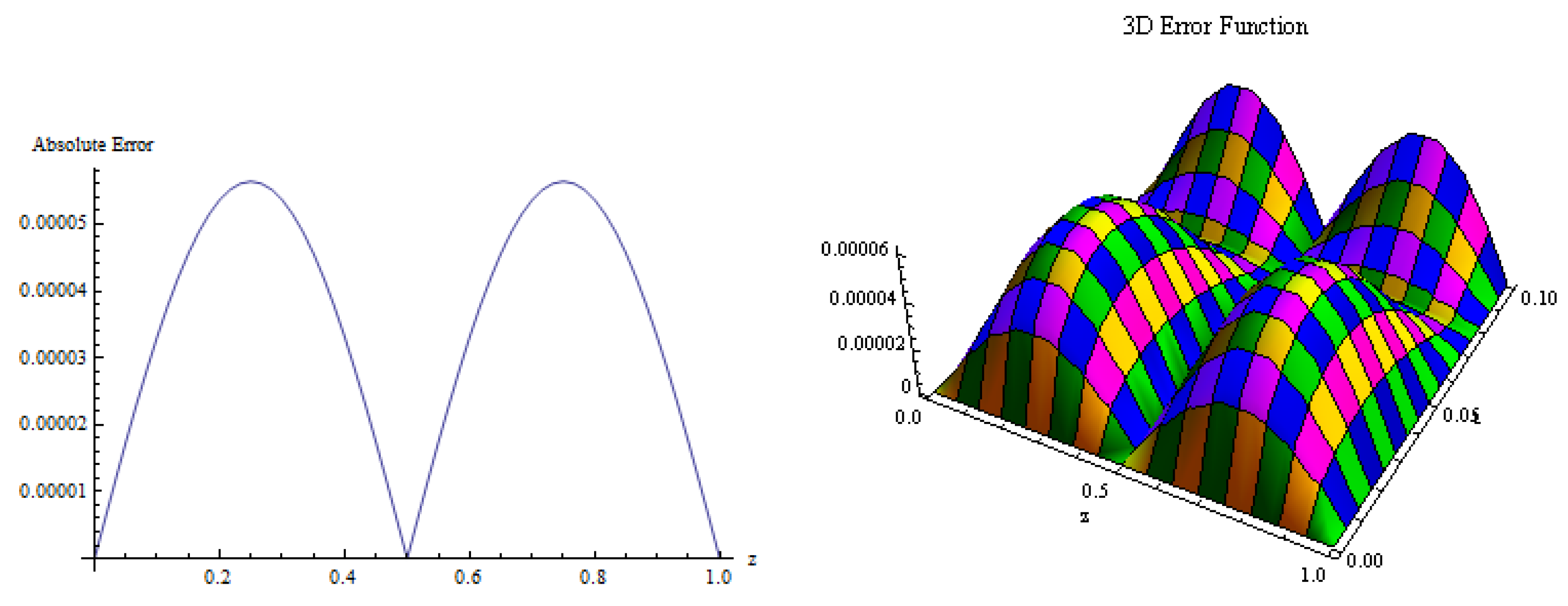
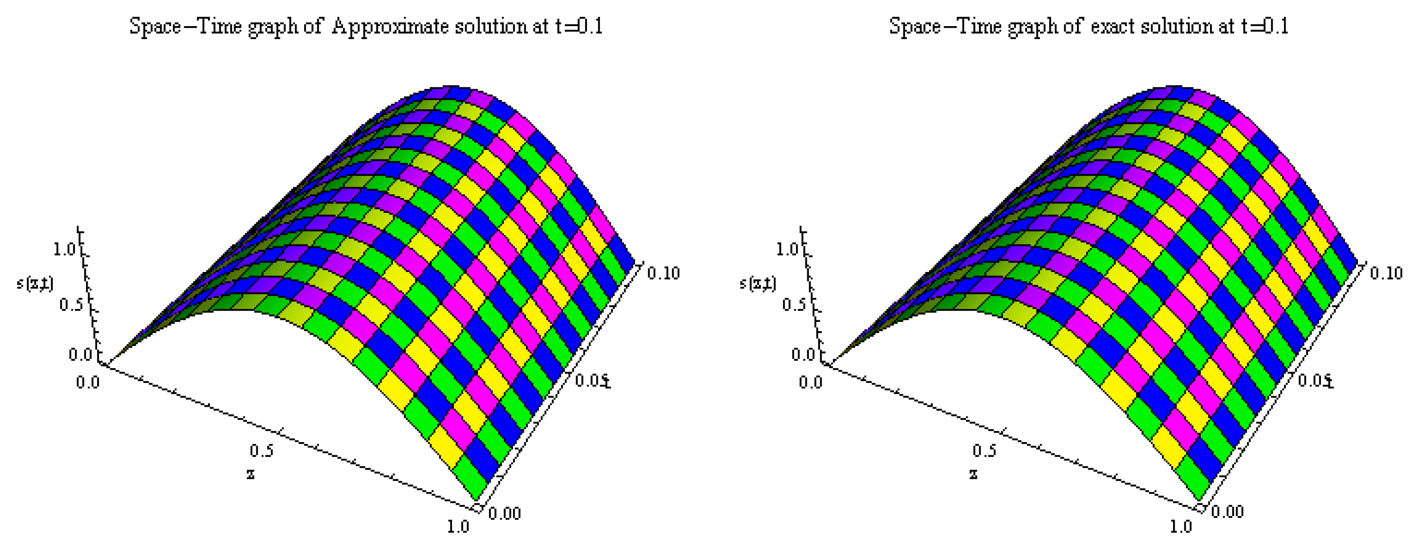
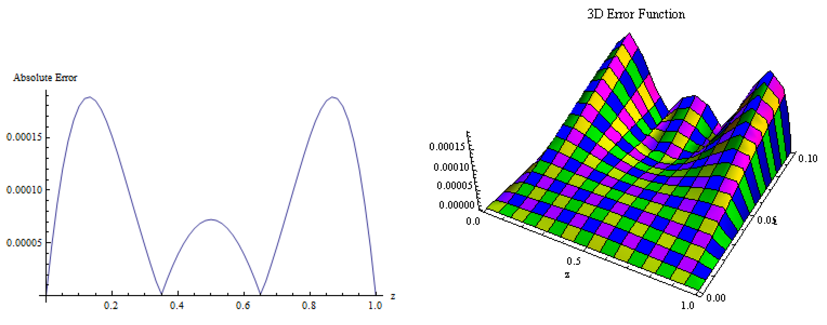
The exact solution of this problem is $s(z,t)=sin\left(\pi z\right)-\frac{4t^{\frac{5}{2}}}{\sqrt{\pi }}sin\left(2\pi z\right)$ with $\psi =\frac{1}{2}$. The introduced scheme is applied to the above problem and the numerical results are acquired using Mathematica 12. In

Table 1. Comparative analysis of errors for Example 1 with $\Delta k={10}^{-5}$ and $N=10$.

Q	NECuBS		TCuBS [20]		CuBS [19]	QBS [18]	QWM [16]
	$L_2$	$L_{\infty }$	$L_2$	$L_{\infty }$	$L_{\infty }$	$L_{\infty }$	$L_{\infty }$
50	8.40 $\times {10}^{-8}$	1.13 $\times {10}^{-7}$	5.96 $\times {10}^{-6}$	8.93 $\times {10}^{-6}$	1.24 $\times {10}^{-6}$	1.18 $\times {10}^{-4}$	1.58 $\times {10}^{-3}$
150	1.48 $\times {10}^{-7}$	2.02 $\times {10}^{-7}$	3.09 $\times {10}^{-5}$	4.42 $\times {10}^{-5}$	6.34 $\times {10}^{-6}$	6.75 $\times {10}^{-4}$	7.89 $\times {10}^{-3}$
250	1.93 $\times {10}^{-7}$	2.62 $\times {10}^{-7}$	6.65 $\times {10}^{-5}$	9.45 $\times {10}^{-5}$	1.36 $\times {10}^{-5}$	1.40 $\times {10}^{-3}$	1.61 $\times {10}^{-2}$
350	2.29 $\times {10}^{-7}$	3.11 $\times {10}^{-7}$	1.10 $\times {10}^{-4}$	1.56 $\times {10}^{-4}$	2.25 $\times {10}^{-5}$	2.51 $\times {10}^{-3}$	2.53 $\times {10}^{-2}$
450	2.59 $\times {10}^{-7}$	3.53 $\times {10}^{-7}$	1.60 $\times {10}^{-4}$	2.28 $\times {10}^{-4}$	3.28 $\times {10}^{-5}$	3.70 $\times {10}^{-3}$	3.46 $\times {10}^{-2}$

, the computed errors of the present scheme are tabulated and compared to those presented in [16,17,18,19] for various time stages. Figure 1 depicts a close comparison of exact and approximate solutions. In Figure 2, 3D error profiles of the approximate and exact solutions are displayed, which shows the exactness of our methodology. Figure 3 displays the error functions for both 2D and 3D cases. The numerical solution for the scenario where $h=0.05$, $t=1$, and $\Delta k=0.01$ is provided as

$$\begin{array}{c}\hfill S(z,1)=\left\{\begin{array}{c}1.73472\times {10}^{-18}-1.53732z+0.0026847z^2+\hfill \\ 4.07744z^3+318.921z^4,\hfill & z\in [0,\frac{1}{20})\hfill \\ 0.0197548-2.79779z+28.2192z^2-244.176z^3+920.358z^4,\hfill & z\in [\frac{1}{20},\frac{1}{10})\hfill \\ 0.311013-12.0329z+130.518z^2-684.653z^3+1417.75z^4,\hfill & z\in [\frac{1}{10},\frac{3}{20})\hfill \\ ⋮\hfill \\ ⋮\hfill \\ -1227.72+5589.46z-9523.68z^2+7211z^3-2049.49z^4,\hfill & z\in [\frac{17}{20},\frac{9}{10})\hfill \\ -990.477+4256.43z-6837.66z^2+4877.41z^3-1305.73z^4,\hfill & z\in [\frac{9}{10},\frac{19}{20})\hfill \\ -446.381+1803.22z-2707.92z^2+1799.53z^3-448.446z^4,\hfill & z\in [\frac{19}{20},1).\hfill \end{array}\right.\end{array}$$

Example 2.

Consider the Equation (1) with exact solution $s(z,t)={(t+1)}^{2}sin\pi z$ subject to initial condition $s(z,0)=sin\pi z$ and boundary conditions $s(0,t)=s(1,t)=0$. Moreover, $p(z,t)$ is to be chosen accordingly when $\psi =0.5$.

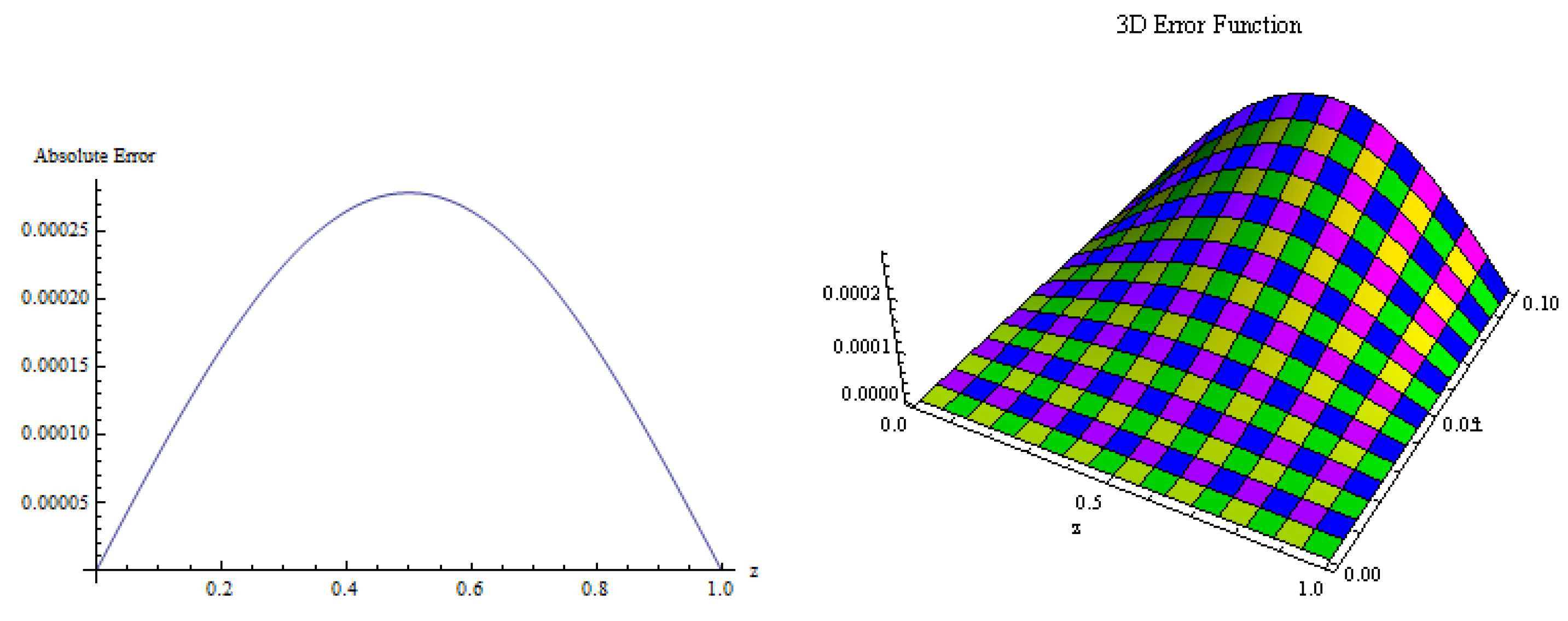
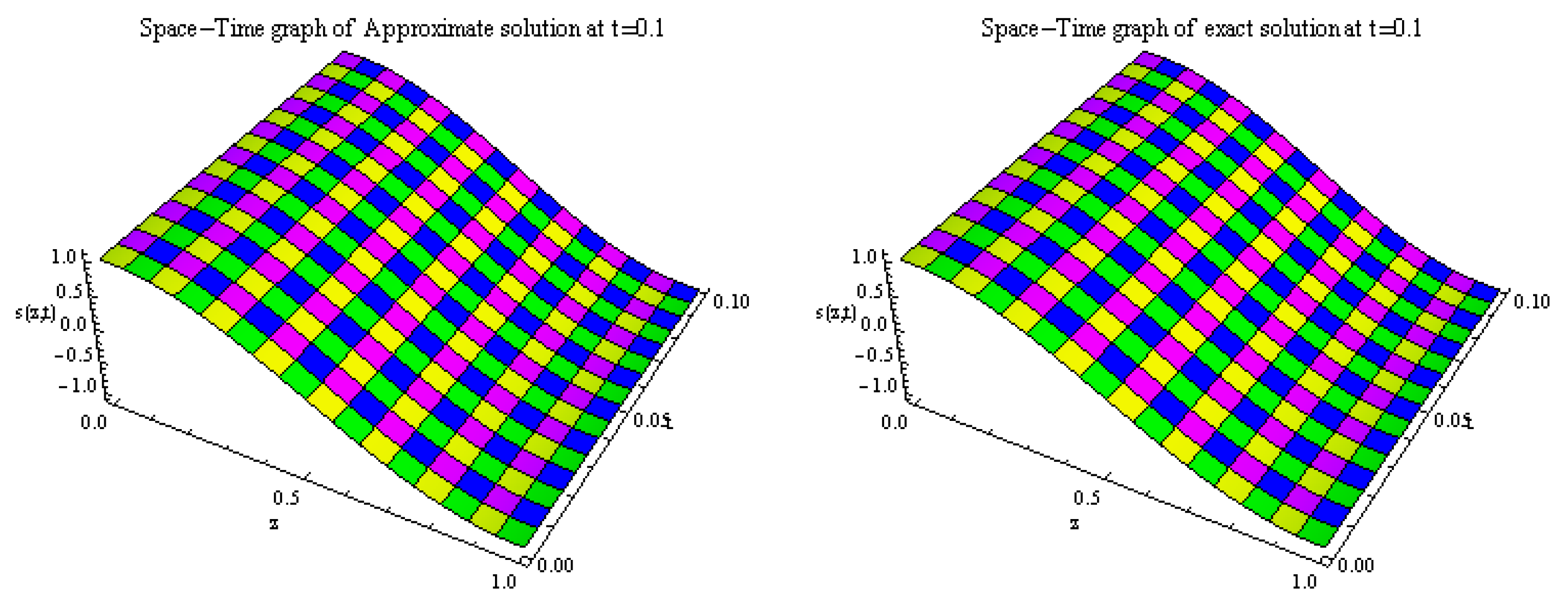
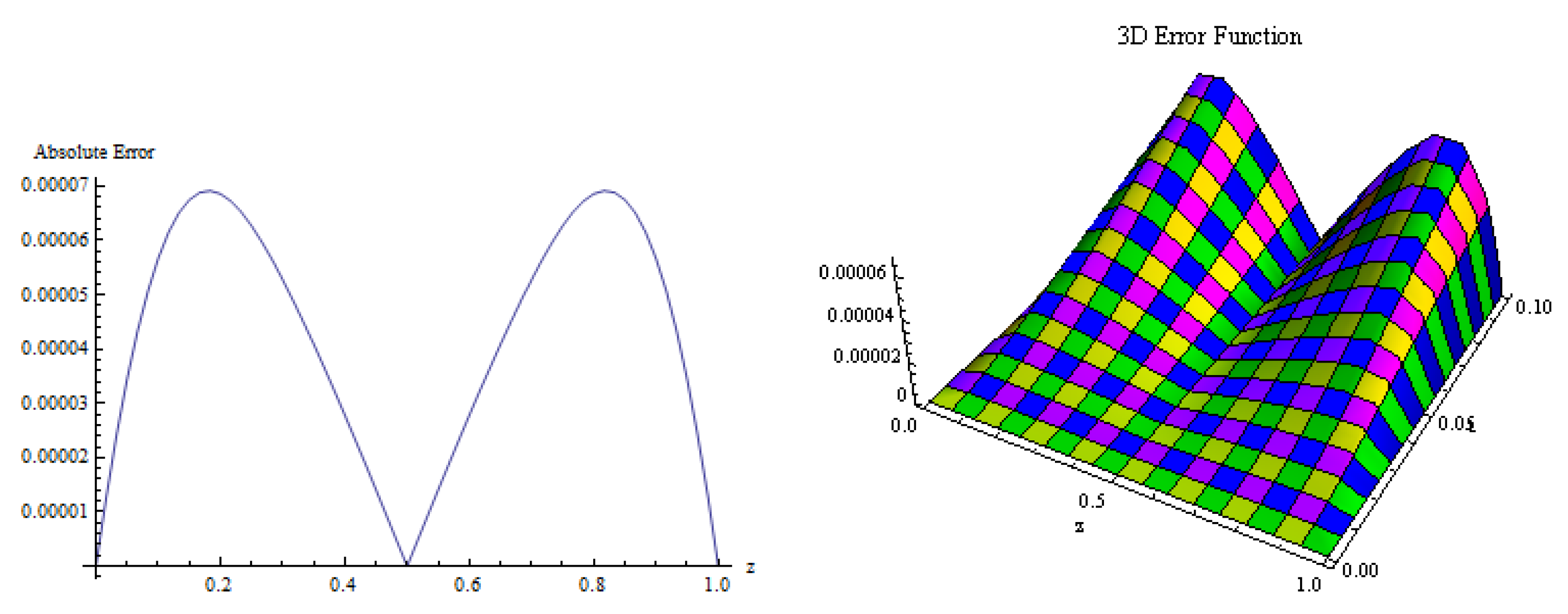
The proposed technique is implemented for the above problem and the approximate solutions are obtained when $h=0.01$, $\Delta k={10}^{-5}$ for optimized value of $\sigma$.

Table 2. Comparative analysis of errors for Example 2 with $h=0.01$ and $\Delta k={10}^{-5}$.

Q	NECuBS		TCuBS [20]		CuBS [19]
	$L_2$	$L_{\infty }$	$L_2$	$L_{\infty }$	$L_2$	$L_{\infty }$
150	5.43 $\times {10}^{-9}$	7.68 $\times {10}^{-9}$	2.82 $\times {10}^{-8}$	3.99 $\times {10}^{-8}$	3.93 $\times {10}^{-8}$	5.56 $\times {10}^{-8}$
200	6.13 $\times {10}^{-9}$	8.67 $\times {10}^{-9}$	4.56 $\times {10}^{-8}$	6.45 $\times {10}^{-8}$	6.26 $\times {10}^{-8}$	8.86 $\times {10}^{-8}$
250	6.43 $\times {10}^{-9}$	9.06 $\times {10}^{-9}$	6.59 $\times {10}^{-8}$	9.31 $\times {10}^{-8}$	8.97 $\times {10}^{-8}$	1.27 $\times {10}^{-8}$
300	6.38 $\times {10}^{-9}$	9.03 $\times {10}^{-9}$	8.86 $\times {10}^{-8}$	1.25 $\times {10}^{-7}$	1.20 $\times {10}^{-7}$	1.70 $\times {10}^{-7}$
350	6.01 $\times {10}^{-9}$	8.50 $\times {10}^{-9}$	1.14 $\times {10}^{-7}$	1.61 $\times {10}^{-7}$	1.53 $\times {10}^{-7}$	2.17 $\times {10}^{-7}$
400	5.34 $\times {10}^{-9}$	7.56 $\times {10}^{-9}$	1.41 $\times {10}^{-7}$	1.99 $\times {10}^{-7}$	1.89 $\times {10}^{-7}$	2.67 $\times {10}^{-7}$

illustrates the comparison between the calculated errors using the presented method and those from the references [18,19] across various time levels. Figure 4 showcases a substantial disparity between the approximated and actual solutions. Furthermore, Figure 5 provides a remarkably close comparison of the 3D graphs between the approximate and exact solutions. The presentation of 2D and 3D errors can be observed in Figure 6. Additionally, the numerical solution for the case where $h=0.05$, $t=1$, and $\Delta k=0.01$ is given as

$$\begin{array}{c}\hfill S(z,1)=\left\{\begin{array}{c}-1.11022\times {10}^{-16}+12.5337z-9.69194\times {10}^{-7}{z}^2-\hfill \\ 61.5212z^3+614.183z^4,\hfill & z\in [0,\frac{1}{20})\hfill \\ 0.0381009+10.096z+54.8197z^2-548.301z^3+1827.33z^4,\hfill & z\in [\frac{1}{20},\frac{1}{10})\hfill \\ 0.637203-9.04529z+269.596z^2-1497.86z^3+2995.54z^4,\hfill & z\in [\frac{1}{10},\frac{3}{20})\hfill \\ ⋮\hfill \\ ⋮\hfill \\ 1758.86-8018.7z+13749.2z^2-10484.3z^3+2995.54z^4,\hfill & z\in [\frac{17}{20},\frac{9}{10})\hfill \\ 1343.99-5784.17z+9373.93z^2-6761.04z^3+1827.33z^4,\hfill & z\in [\frac{9}{10},\frac{19}{20})\hfill \\ 565.196-2284.7z+3500.54z^2-2395.21z^3+614.183z^4,\hfill & z\in [\frac{19}{20},1).\hfill \end{array}\right.\end{array}$$

Example 3.

Consider (1) with exact solution

$$s(z,t)=(t+1)cos\pi z,z\in [0,1].$$

(52)

The assessment of initial and boundary conditions is based on Equation (52). The selection of the function $p(z,t)$ should align accordingly.

The introduced methodology is employed for the above problem to obtain the approximate solution. The computed errors of the presented scheme are compared with those presented in [18,19] for $h=0.05$, $\Delta t={10}^{-4}$, $\psi =\frac{1}{3}$, and for optimized value of $\sigma$ for Example 3 in

Table 3. Comparative analysis of errors for Example 3 with $h=0.05$ and $\Delta k={10}^{-4}$.

Q	NECuBS		TCuBS [20]		CuBS [19]
	$L_2$	$L_{\infty }$	$L_2$	$L_{\infty }$	$L_2$	$L_{\infty }$
50	4.42 $\times {10}^{-8}$	1.73 $\times {10}^{-8}$	2.73 $\times {10}^{-7}$	4.19 $\times {10}^{-7}$	3.48 $\times {10}^{-7}$	5.34 $\times {10}^{-7}$
100	1.39 $\times {10}^{-7}$	1.73 $\times {10}^{-7}$	8.48 $\times {10}^{-7}$	1.26 $\times {10}^{-6}$	1.08 $\times {10}^{-6}$	1.61 $\times {10}^{-6}$
150	2.70 $\times {10}^{-7}$	1.73 $\times {10}^{-7}$	1.64 $\times {10}^{-6}$	2.42 $\times {10}^{-6}$	2.09 $\times {10}^{-6}$	3.08 $\times {10}^{-6}$
200	4.31 $\times {10}^{-7}$	6.27 $\times {10}^{-7}$	2.61 $\times {10}^{-6}$	3.82 $\times {10}^{-6}$	3.33 $\times {10}^{-6}$	4.87 $\times {10}^{-6}$
250	6.16 $\times {10}^{-7}$	9.04 $\times {10}^{-7}$	3.73 $\times {10}^{-6}$	5.51 $\times {10}^{-6}$	4.76 $\times {10}^{-6}$	7.02 $\times {10}^{-6}$
300	8.24 $\times {10}^{-7}$	1.20 $\times {10}^{-6}$	4.99 $\times {10}^{-6}$	7.33 $\times {10}^{-6}$	6.36 $\times {10}^{-6}$	9.35 $\times {10}^{-6}$

. In Figure 7, a close contrast of exact and approximate solutions is depicted, while 3D comparison of exact and approximate solutions is plotted in Figure 8. The graphs are in tremendous affirmation. Figure 9 shows the 2D and 3D error graphs. The following numerical solution corresponds to the values $h=0.05$, $t=1$, and $\Delta k=0.01$.

$$\begin{array}{c}\hfill S(z,1)=\left\{\begin{array}{cc}2-0.0101225z-0.48932z^2-373.465z^3+3735.06z^4,\hfill & z\in [0,\frac{1}{20})\hfill \\ 2.09164-5.49694z+108.786z^2-1092.76z^3+3642.92z^4,\hfill & z\in [\frac{1}{20},\frac{1}{10})\hfill \\ 2.78381-26.0803z+310.986z^2-1730.41z^3+3461.22z^4,\hfill & z\in [\frac{1}{10},\frac{3}{20})\hfill \\ ⋮\hfill \\ ⋮\hfill \\ -2018.49+9249.53z-15887.1z^2+12114.5z^3-3461.22z^4,\hfill & z\in [\frac{17}{20},\frac{9}{10})\hfill \\ -2655.54+11505.5z-18688z^2+13478.9z^3-3642.92z^4,\hfill & z\in [\frac{9}{10},\frac{19}{20})\hfill \\ -3363.09+13818.8z-21289.5z^2+14566.8z^3-3735.06z^4,\hfill & z\in [\frac{19}{20},1).\hfill \end{array}\right.\end{array}$$

Example 4.

Consider (1) with initial condition

$$s(z,0)=2{sin}^2\pi z,$$

and the boundary conditions

$$s(0,t)=0,s(1,t)=0.$$

This equation has the exact solution

$$s(z,t)=2(t^2+t+1){sin}^2\pi z,$$

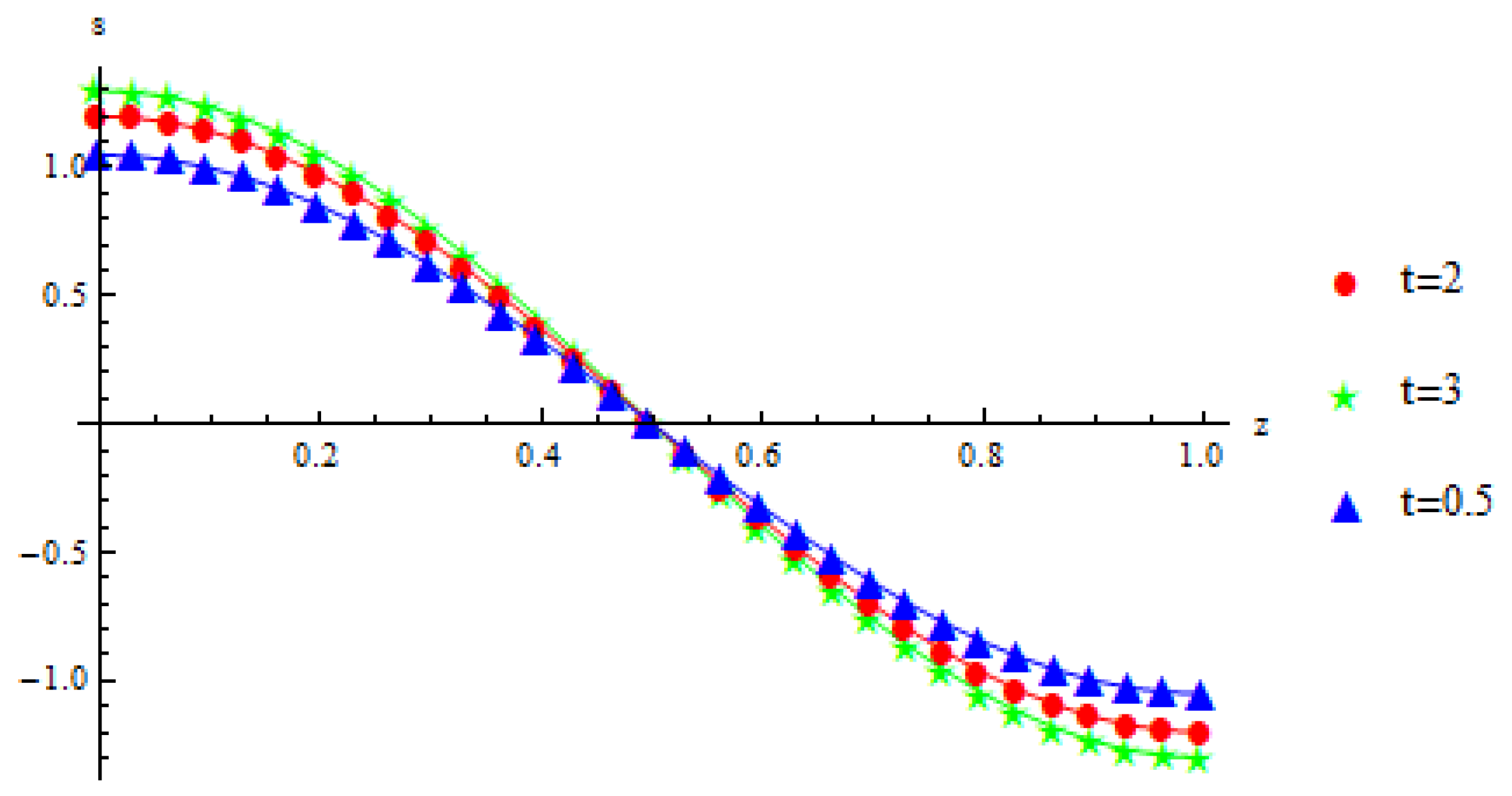
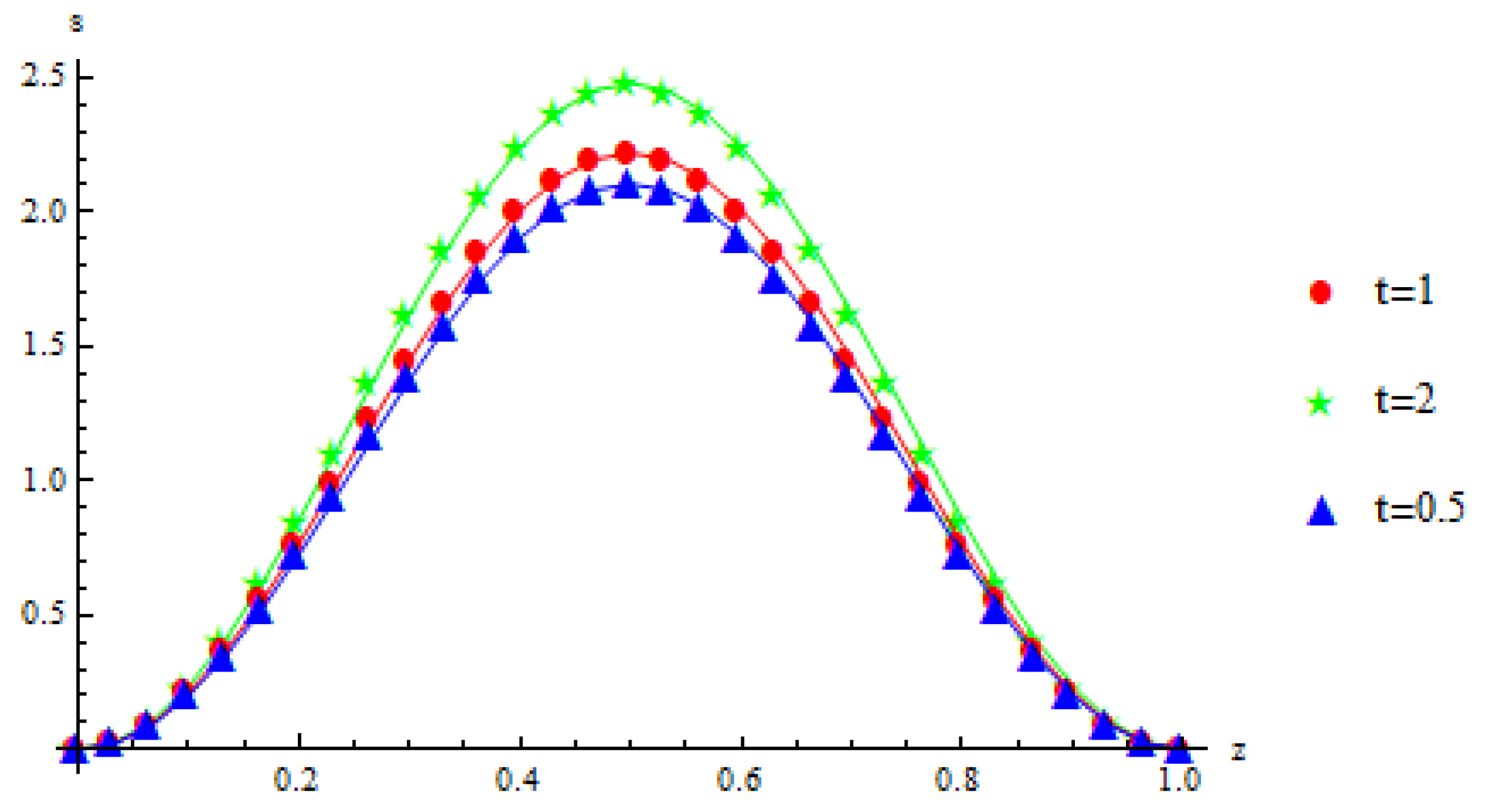
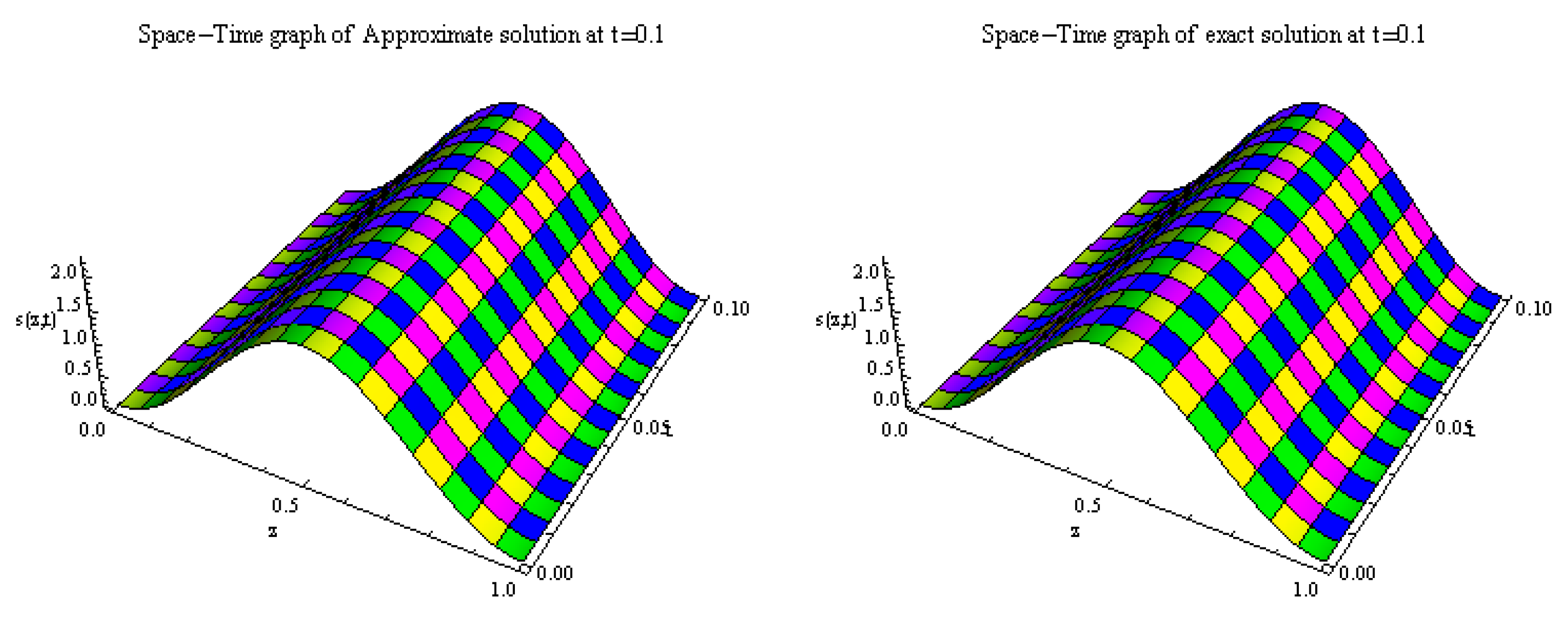
$p(z,t)$ is to be chosen with $\psi =\frac{1}{4}$. The offered scheme is implemented to obtain the numerical results of Example 4. Errors of the proposed algorithm for $h=0.05$, $\Delta k=0.0001$, and $Q=50,100,\dots ,300$ are evaluated.

Table 4. Comparison of errors and assessment of error norms for Example 4 with $h=0.05$ and $\Delta k=0.0001$.

Q	NECuBS		TCuBS [20]		CuBS [19]
	$L_2$	$L_{\infty }$	$L_2$	$L_{\infty }$	$L_2$	$L_{\infty }$
50	5.58 $\times {10}^{-7}$	8.51 $\times {10}^{-7}$	2.29 $\times {10}^{-6}$	4.26 $\times {10}^{-6}$	2.46 $\times {10}^{-6}$	4.53 $\times {10}^{-6}$
100	1.06 $\times {10}^{-6}$	1.50 $\times {10}^{-6}$	7.89 $\times {10}^{-6}$	1.24 $\times {10}^{-5}$	8.44 $\times {10}^{-6}$	1.32 $\times {10}^{-5}$
150	1.52 $\times {10}^{-6}$	1.97 $\times {10}^{-6}$	1.61 $\times {10}^{-5}$	2.50 $\times {10}^{-5}$	1.72 $\times {10}^{-5}$	2.67 $\times {10}^{-5}$
200	1.97 $\times {10}^{-6}$	2.29 $\times {10}^{-6}$	2.66 $\times {10}^{-5}$	3.94 $\times {10}^{-5}$	2.84 $\times {10}^{-5}$	4.19 $\times {10}^{-5}$
250	2.43 $\times {10}^{-6}$	2.53 $\times {10}^{-6}$	3.90 $\times {10}^{-5}$	5.74 $\times {10}^{-5}$	4.17 $\times {10}^{-5}$	6.12 $\times {10}^{-5}$
300	2.89 $\times {10}^{-6}$	3.43 $\times {10}^{-6}$	5.33 $\times {10}^{-5}$	7.76 $\times {10}^{-5}$	5.69 $\times {10}^{-5}$	8.29 $\times {10}^{-5}$

compares calculated errors of the present scheme with those computed in [18,19]. Figure 10 plots an excellent comparison of approximate and exact solutions for different times. Figure 11 displays the three-dimensional comparison between the approximate and exact solutions. The visualization of both the 2D and 3D error functions is presented in Figure 12. Additionally, the numerical solution corresponding to $h=0.05$, $t=1$, and $\Delta k=0.01$ is given by

$$\begin{array}{c}\hfill S(z,1)=\left\{\begin{array}{c}3.46945\times {10}^{-18}-0.0136697z+0.299777z^2+\hfill \\ 2326.44z^3-23265.4z^4,\hfill & z\in [0,\frac{1}{20})\hfill \\ -0.538757+32.0261z-629.067z^2+6293.66z^3-20979.8z^4,\hfill & z\in [\frac{1}{20},\frac{1}{10})\hfill \\ -3.86934+127.617z-1498.46z^2+8326.4z^3-16653.7z^4,\hfill & z\in [\frac{1}{10},\frac{3}{20})\hfill \\ ⋮\hfill \\ ⋮\hfill \\ -9702+44504.9z-76441.4z^2+58288.4z^3-16653.7z^4,\hfill & z\in [\frac{17}{20},\frac{9}{10})\hfill \\ -15283.7+66264.4z-107627z^2+77625.6z^3-20979.8z^4,\hfill & z\in [\frac{9}{10},\frac{19}{20})\hfill \\ -20938.6+86081.5z-132613z^2+90735z^3-23265.4z^4,\hfill & z\in [\frac{19}{20},1).\hfill \end{array}\right.\end{array}$$

6. Conclusions

This study presents an innovative extended cubic B-spline collocation technique as a powerful numerical tool for addressing second-order PIDE. Our proposed approach harnesses the flexibility and accuracy of B-spline functions, providing an effective means of approximating solutions to Volterra PIDEs. A new extended B-spline-based approximation is used to approximate second-order spatial derivatives. The temporal derivatives are discretized by the finite difference formula. The suggested scheme’s stability and convergence analysis are provided to substantiate accuracy and validity. As the understanding of dynamic processes with memory effects continues to grow in importance across various domains, the need for efficient and reliable numerical techniques for solving Volterra PIDEs becomes increasingly crucial. We believe that our proposed method can contribute significantly to advancing research in these areas. The obtained results show that the proposed method offers high accuracy and robustness, making it a valuable addition to the toolkit of researchers and practitioners working in fields where Volterra PIDEs play a significant role. The obtained results are compared with those acquired using TCuBS, CuBS, QBS, and QWM already available in the literature.

References

1. Lakshmikantham, V.; Rama, M. Theory of Integro-Differential Equations; CRC Press: Boca Raton, FL, USA, 1995. [Google Scholar]
2. Thiem, H.R. A model for spatio spread of an epidemic. Math. Biol. 1977, 4, 337–351. [Google Scholar] [CrossRef] [PubMed]
3. Sloan, I.; Thome, V. Time Discretization of an Integro-Differential Equation of Parabolic Type. SIAM J. Numer. Anal. 1986, 23, 1052–1061. [Google Scholar] [CrossRef]
4. Shakeri, F.; Dehghan, M. A high order finite volume element method for solving elliptic partial integro-differential equations. Appl. Numer. Math. 2013, 65, 105–118. [Google Scholar] [CrossRef]
5. Cushing, J.M. Integrodifferential Equations and Delay Models in Population Dynamics; Springer: Berlin/Heidelberg, Germany, 1977. [Google Scholar]
6. Lin, Y.; Xu, C. Finite difference/spectral approximations for the time-fractional diffusion equation. J. Comput. Phys. 2007, 225, 1533–1552. [Google Scholar] [CrossRef]
7. Dehghan, M.; Salehi, R. The numerical solution of the non-linear integro-differential equations based on the meshless method. J. Comput. Appl. Math. 2012, 236, 2367–2377. [Google Scholar] [CrossRef]
8. McLean, W.; Thome, V. Numerical solution of an evolution equation with a positive-type memory term. J. Aust. Math. Soc. Ser. B 1993, 35, 23–70. [Google Scholar] [CrossRef]
9. Desch, W.; Grimmer, R.; Schappacher, W. Some considerations for Linear integrodifferential equations. J. Math. Anal. 1984, 104, 219–234. [Google Scholar] [CrossRef]
10. Day, J.T. Note on the numerical solution of Integro-Differential equations. J. Comput. 1967, 9, 394–395. [Google Scholar] [CrossRef]
11. Ebadi, G.; Rahimiardabili, M.; Shahmorad, S. Numerical solution of the nonlinear Volterra integro-differential equations by the tau method. Appl. Math. Comput. 2007, 188, 1580–1586. [Google Scholar]
12. Siraj-ul-Islam, A.I.; Fayyaz, M. A new approach for numerical solution of integro-differential equations via Haar wavelets. Int. J. Comput. Math. 2013, 90, 1971–1989. [Google Scholar] [CrossRef]
13. Von Petersdorff, T.; Schwab, C. Wavelet discretizations of parabolic integrodifferential equations. SIAM J. Numer. Anal. 2003, 41, 159–180. [Google Scholar] [CrossRef]
14. Zalik, R.; Vinogradov, A. The Quasi-Elastic method of solution for a class of integrodifferential equations. J. Integral Equ. Appl. 1993, 5, 277–295. [Google Scholar] [CrossRef]
15. Rostami, Y.; Maleknejad, K. Numerical solution of partial Integro-Differential equations by using projection method. Mediterr. J. Math. 2017, 14, 113. [Google Scholar] [CrossRef]
16. Long, W.T.; Xu, D.; Zeng, X.Y. Quasi wavelet based numerical method for a class of partial integro-differential equation. Appl. Math. Comput. 2012, 218, 11842–11850. [Google Scholar] [CrossRef]
17. Akram, T.; Abbas, M.; Riaz, M.B.; Ismail, A.I.; Ali, N.H.M. Development and analysis of new approximation of extended cubic b-spline to the nonlinear time fractional klein–gordon equation. Fractals 2020, 28, 2040039. [Google Scholar] [CrossRef]
18. Ali, A.; Ahmad, S.; Shah, S.I.; Haq, F. A Quartic B-spline collocation technique for the solution of partial integro-differential equations with a weakly kernel. Sci. Int. 2015, 27, 2953–2958. [Google Scholar]
19. Gholamian, M.; Saberi-Nadjafi, J. Cubic B-splines collocation method for a class of partial integro-differential equation. Alex. Eng. J. 2017, 57, 2157–2165. [Google Scholar] [CrossRef]
20. Ali, A.; Khan, K.; Haq, F.; Shah, S.I. A Computational Modeling Based on Trigonometric Cubic B-Spline Functions for the Approximate Solution of a Second Order Partial Integro-Differential Equation. In World Conference on Information Systems and Technologies; Rocha, Á., Adeli, H., Reis, L., Costanzo, S., Eds.; Springer International Publishing: Cham, Switzerland, 2019; Volume 930, pp. 844–854. [Google Scholar]
21. de Boor, C. On the convergence of odd degree spline interpolation. J. Approx. Theory 1968, 1, 452–463. [Google Scholar] [CrossRef]
22. Hall, C.A. On error bounds for spline interpolation. J. Approx. Theory 1968, 1, 209–218. [Google Scholar] [CrossRef]
23. Prenter, P.M. Spline and Variational Methods; Wiley: New York, NY, USA, 1975. [Google Scholar]
24. Akram, T.; Abbas, M.; Ismail, A.I.; Ali, N.H.M.; Baleanu, D. Extended cubic B-splines in the numerical solution of time fractional telegraph equation. Adv. Differ. Equ. 2019, 2019, 365. [Google Scholar] [CrossRef]
25. Wasim, I.; Abbas, M.; Iqbal, K.I. A new extended B-spline approximation technique for second order singular boundary value problems arising in physiology. J. Math. Comput. Sci. 2019, 19, 258–267. [Google Scholar] [CrossRef]
26. Stoer, J.; Bulirsch, R. Introduction to Numerical Analysis, 3rd ed.; Springer: New York, NY, USA, 2002. [Google Scholar]
Figure 1. Exact and estimated solutions (represented by triangles, stars, and circles) for Example 1 at different time instances, with a fixed value of h = 0.01 .
Symmetry 15 01851 g001
Figure 2. Approximated solution (on the left) and precise solution (on the right) for Example 1 under the conditions h = 1 60 , t = 0.1 , and Δ k = 0.01 .
Symmetry 15 01851 g002
Figure 3. Error patterns in both two-dimensional and three-dimensional contexts for Example 1 under the parameter settings h = 1 60 , t = 0.1 , and Δ k = 0.01 .
Symmetry 15 01851 g003
Figure 4. Exact and estimated solutions (represented by triangles, stars, and circles) for Example 2 at different time instances with a fixed value of h = 0.01 .
Symmetry 15 01851 g004
Figure 5. Approximated solution (on the left) and exact solution (on the right) for Example 2 under the conditions h = 1 60 , t = 0.1 , and Δ k = 0.01 .
Symmetry 15 01851 g005
Figure 6. Error profiles in both two-dimensional and three-dimensional contexts for Example 2 under the parameter settings h = 1 60 , t = 0.1 , and Δ k = 0.01 .
Symmetry 15 01851 g006
Figure 7. Exact and estimated (depicted by triangles, stars, and circles) solutions for Example 3 across different time points with a step size of h = 0.01 .
Symmetry 15 01851 g007
Figure 8. Approximated solution (on the left) and accurate solution (on the right) for Example 3 under the conditions h = 1 60 , t = 0.1 , and Δ k = 0.01 .
Symmetry 15 01851 g008
Figure 9. The estimated solution (on the left) and the exact solution (on the right) for Example 3 with h = 1 60 , t = 0.1 , and Δ k = 0.01 .
Symmetry 15 01851 g009
Figure 10. Exact and estimated (indicated by triangles, stars, and circles) solutions for Example 4 at different time instances with a step size of h = 0.01 .
Symmetry 15 01851 g010
Figure 11. The approximated solution (on the left) and the exact solution (on the right) for Example 4 under the conditions h = 1 60 , t = 0.1 , and Δ k = 0.01 .
Symmetry 15 01851 g011
Figure 12. Two-dimensional and three-dimensional representations of error profiles for Example 4 with the parameter values h = 1 60 , t = 0.1 , and Δ k = 0.01 .
Symmetry 15 01851 g012