Improving Performance of Differential Evolution Using Multi-Population Ensemble Concept

Abstract

Differential evolution (DE) stands out as a straightforward yet remarkably powerful evolutionary algorithm employed for real-world problem-solving purposes. In the DE algorithm, few parameters are used, and the population is evolved by applying various operations. It is difficult in evolutionary computation algorithms to maintain population diversity. The main issue is the sub-population of the DE algorithm that helps improve convergence speed and escape from the local optimum. Evolving sub-populations by maintaining diversity is an important issue in the literature that is considered in this research. A solution is proposed that uses sub-populations to promote greater diversity within the population and improve the algorithm performance. DE, heterogeneous distributed differential evolution (HDDE), multi-population ensemble differential evolution (MPEDE), and the proposed improved multi-population ensemble differential evolution (IMPEDE) are implemented using parameter settings; population sizes of 100 NP, 150 NP, and 200 NP; and dimensions of 10D, 30D, and 50D for performance comparison. Different combinations of mutations are used to generate the simulated results. The simulation results are generated using 1000, 3000, and 5000 iterations. Experimental outcomes show the superior results of the proposed IMPEDE over existing algorithms. The non-parametric significance Friedman test confirms that there is a significant difference in the performance of the proposed algorithm and other algorithms used in this study by considering a 0.05 level of significance using six benchmark functions.

1. Introduction

Optimization is the process of obtaining the best value decision variables for a given set of constraints [1]. Today, optimization is considered a very important area of research to solve real-world problems in engineering, business, industry, and computer science. Evolutionary algorithms have been widely adopted in different domains and are considered to be very effective in solving real-world optimization problems [2]. A number of evolutionary algorithms and their variants have been introduced in the last decade [3]. The differential evolution (DE) algorithm is considered to be one of the most powerful evolutionary computing algorithms to solve real-world problems. Price and Storn [4] proposed the DE algorithm in 1995 as a simple yet very powerful stochastic searching technique. DE uses a few control parameters, which is its remarkable advantage [5]. Evolutionary computation algorithms are better at searching for global optima than conventional optimization techniques [6]. The DE algorithm has a strong searching capability that is helpful in providing good-quality solutions to many real-world problems. The DE algorithm employs three control parameters: population size (NP), scaling factor (F), and crossover rate (CR). The DE algorithm uses several mutation strategies [7]. Various mutation strategies are used for global convergence to achieve effective results; some are used in local search for effective results, while others are used to achieve results for various problems [8].

In classical DE, a single mutation strategy and fixed control parameters are used. The performance of the DE algorithm varies across different optimization problems, even when the same set of control parameters and a mutation strategy involving a single offspring generation are used. Furthermore, for the same optimization problem, DE uses the best suitable mutation strategy and suitable control parameters that give effective and high performance [9]. The DE algorithm is applied to several real-life applications, such as clustering, deoxyribonucleic acid (DNA) microarray, and other soft computing techniques [10]. Therefore, the performance of DE mutation strategies differs depending on the specific problem and is sensitive to dimensions. The DE algorithm is a powerful and uncomplicated evolutionary algorithm (EA) that yields highly effective results. It has been successfully used in many optimization problems and soft computing techniques [11]. The simplicity of the differential evolution algorithm uses mutation, crossover, and selection operations that make it competitive with other EAs to achieve effective results, and those operations also guide the EA population to achieve high performance. The DE algorithm has also been successfully applied to solve many other real-world problems in chemical engineering [12], economic dispatch problems [13], gene coevolution [14], circuit parameter optimizations [15], power systems [16], medical imaging [17], and function optimization [18].

Dividing the main population into sub-populations is an important aspect of the DE algorithm. The mechanism of dividing the main population into sub-populations is important in order to obtain better fitness, ensure diversity, escape from local optima, and improve the convergence speed of the DE algorithm. In this study, instead of calculating the best individual, worst individual, and random formation of sub-populations, the average fitness information of the whole population is utilized, which shows significant improvement in the performance of the multi-population-based ensemble DE algorithm.

1.1. Problem Statement

A multi-population-based ensemble DE algorithm utilizes the user-defined number of sub-populations and the random partition of sub-populations that decreases the population diversity. The calculation of the best and worst individual in each iteration is time-consuming. Moreover, a reduction in population diversity results in premature population convergence and slows down the convergence speed.

1.2. Research Questions and Research Hypothesis

The following questions are answered in this study:

• How can the performance of the multi-population-based ensemble DE algorithm be improved by modifying the random partition of sub-populations and the user-defined number of sub-populations?
• How can the performance of the proposed algorithm be assessed using standard benchmark functions?
• Is there a significant difference between the performance of an improved multi-population-based ensemble DE algorithm and other state-of-the-art algorithms?

1.3. Research Contribution

This study makes the following major contributions:

• The number of total sub-populations in the multi-population-based ensemble DE algorithm is enhanced by utilizing fitness-based information of the whole population.
• Experimental results are generated to check the solution quality and convergence speed by considering the test suit of standard benchmark functions and comparing the result with four state-of-the-art algorithms.
• Statistical significance analysis is performed to assess the significance of the proposed algorithm with existing state-of-the-art algorithms.

The remaining paper is organized as follows: The working of the DE algorithm is described in Section 2. A literature review is presented in Section 3, while the proposed approach is discussed in Section 4. Section 5 contains the results and discussions, as well as the statistical results. A conclusion is given in the last section of this paper.

2. Working of DE Algorithm

DE has proven to be an effective and efficient algorithm for real optimization problems, and it shows better performance as compared to another EA-like genetic algorithm (GA). It generates a randomly distributed population, $NP$, of feasible solutions $\left(X_G\right)=\left(\{P_{1,G},P_{2,G},\dots ,P_{NP,G}\}\right)$. Population objects are called individuals and single individuals are $(P_{i,G}=x_{i,G}^1,x_{i,G}^2,\dots ,x_{i,G}^D,i=1,2,\dots ,NP)$, which is used in the DE algorithm, where, in individual, D is the number of dimensions and G denotes the number of generations in a single individual. In individuals, each dimension is initialized randomly in a range [$(X_{min},X_{max})$], where $(X_{min}=x_{min}^1,x_{min}^2,\dots ,x_{min}^D)$ and $(X_{max}=x_{max}^1,x_{max}^2,\dots ,x_{max}^D)$.

2.1. Mutation

In the DE algorithm, a mutation strategy is used to generate a donor/mutant vector. Therefore, the differential evolution algorithm contains different vectors and a parent vector by using different vectors/individuals. In mutation strategy, it generates a parent vector by using different other vectors; the different vector is selected with different techniques and must be a distant vector. A simple mutation strategy selects three other distinct vectors. Vectors are commonly represented by DE/$x/y/z$, where the base vector is represented by x (is called a base vector), difference vectors are represented by y, and crossover is represented by z. Constant F is an amplification factor that real factor is used to scale the difference vector. The differential evolution classical algorithm uses DE/rand/1 for mutant vector generation.

$$V_{i,G}=X_{a,G}+F\ast \left(X_{b,G}-X_{c,G}\right),a\ne b\ne c$$

(1)

where $(X_{a,G},X_{b,G})$ and $\left(X_{c,G}\right)$ are vectors selected from the current population, the target individual is $\left(X_{i,G}\right)$, and $(X_{a,G},X_{b,G})$ and $\left(X_{c,G}\right)$ are three random individuals.

The best fitness values of the current generation, G, is represented by $\left(X_{best,G}\right)$. $(X_{a,G},X_{b,G},X_{c,G},X_{d,G})$ and $\left(X_{e,G}\right)$ are five individuals that are randomly selected from the current population, while $\left(X_{i,G}\right)$ is the target vector.

2.2. Crossover Operation

The use of the crossover operation in differential evolution contributes to enhancing the diversity within the population. It is used to select the offspring vector. Next, this vector is used in the selection parameter. Crossover operations use the following equation to create a trail vector:

$$U_{b,G}=\left\{\begin{array}{cc}{V}_{b,G},\hfill & \mathit{if}ran{d}_j(0,1)\le C_{r}orj=j_{rand}\hfill \\ X_{b,G},\hfill & otherwise\hfill \end{array}\right.$$

(2)

The types of crossover are discussed as follows.

2.2.1. Binomial Crossover

Binomial crossover, also called uniform crossover, is a process of crossover in which offspring vector, U, is taken from mutant vector, V, and the current vector of population, X, by using crossover probability, $C_r$. Binomial crossover is described in  Algorithm 1.

Algorithm 1 Binomial crossover.

1: $\mathbf{crossoveBin}\left(X,V\right)$ 2: $k\leftarrow irand\left(\left\{1,2,\dots ,n\right\}\right)$ 3: for  $m\in \{1,2,\dots ,n\}$do 4:    if $rand\left(0,1\right)<C_r\mathbf{or}m=k$ then 5:      $U_m=V_m$ 6:    else 7:      $U_m=X_m$ 8:    end if 9: end for 10: return  U

2.2.2. Exponential Crossover

Exponential crossover is a crossover process in which choosing an offspring vector is carried out by comparing each parameter randomly. The trail vector is generated from the base vector or mutant vector and compared in every dimension. In the end, the offspring may be completely different from the trail vector and mutant vector. In an exponential crossover with a two-point crossover, the first point is selected randomly from $\left\{1,2,\dots ,n\right\}$ and the second point is selected by using L consecutive components from mutant which is described in Algorithm 2.

Algorithm 2 Exponential crossover.

1: $\mathbf{crossoveExp}\left(X,V\right)$ 2: $U\leftarrow X;k\leftarrow irand\left(\left\{1,2,\dots ,n\right\}\right);j\leftarrow k;L\leftarrow 0$ 3: while  $rand\left(0,1\right)>C_r\mathbf{or}L=n$  do 4:    $U_j=V_j;j\leftarrow {〈j+1〉}_n;L\leftarrow L+1$ 5: end while 6: return  U

2.2.3. Selection Operation

During the selection operation, a greedy process is employed to choose the best vector that connects the target vector and the trial vector [19]. The selected vector is incorporated as an individual in the next generation. The improvement in algorithm performance is directly influenced by the selection strategies that are employed. To enhance the convergence performance of the algorithm, a well-designed selection strategy is utilized [20]. The selection operation uses the following equation to create a base vector for the next generation:

$$X_{j,G+1}=\left\{\begin{array}{cc}{U}_{j,G}\hfill & \mathit{if}f\left(U_{j,G}\right)\le f\left(X_{j,G}\right)\hfill \\ X_{j,G}\hfill & otherwise\hfill \end{array}\right.$$

(3)

where $j=1,\dots ,NP$ and f represents a fitness function.

The new individual is generated through a series of mutation, crossover, and selection operations by comparing previous vectors, which will be used as a base vector in the next-generation population.

The rest of the paper is organized as follows: A brief overview of the existing literature is discussed in Section 3. The proposed algorithm is presented in Section 4. Section 5 is about the results and discussions of the proposed algorithm. In the end, the study is concluded in Section 6.

3. Literature Review

A detailed literature review of DE is presented by analyzing a number of research papers that are related to DE and other EAs. Many schemes that are used in DE are discussed here. The differential evolution algorithm runs on populations, and the performance is directly affected by the population size [7]. To enhance the algorithm’s performance, the population must be diversified. Various approaches for population enhancement in differential evolution are used by many researchers.

3.1. Single-Population Approach

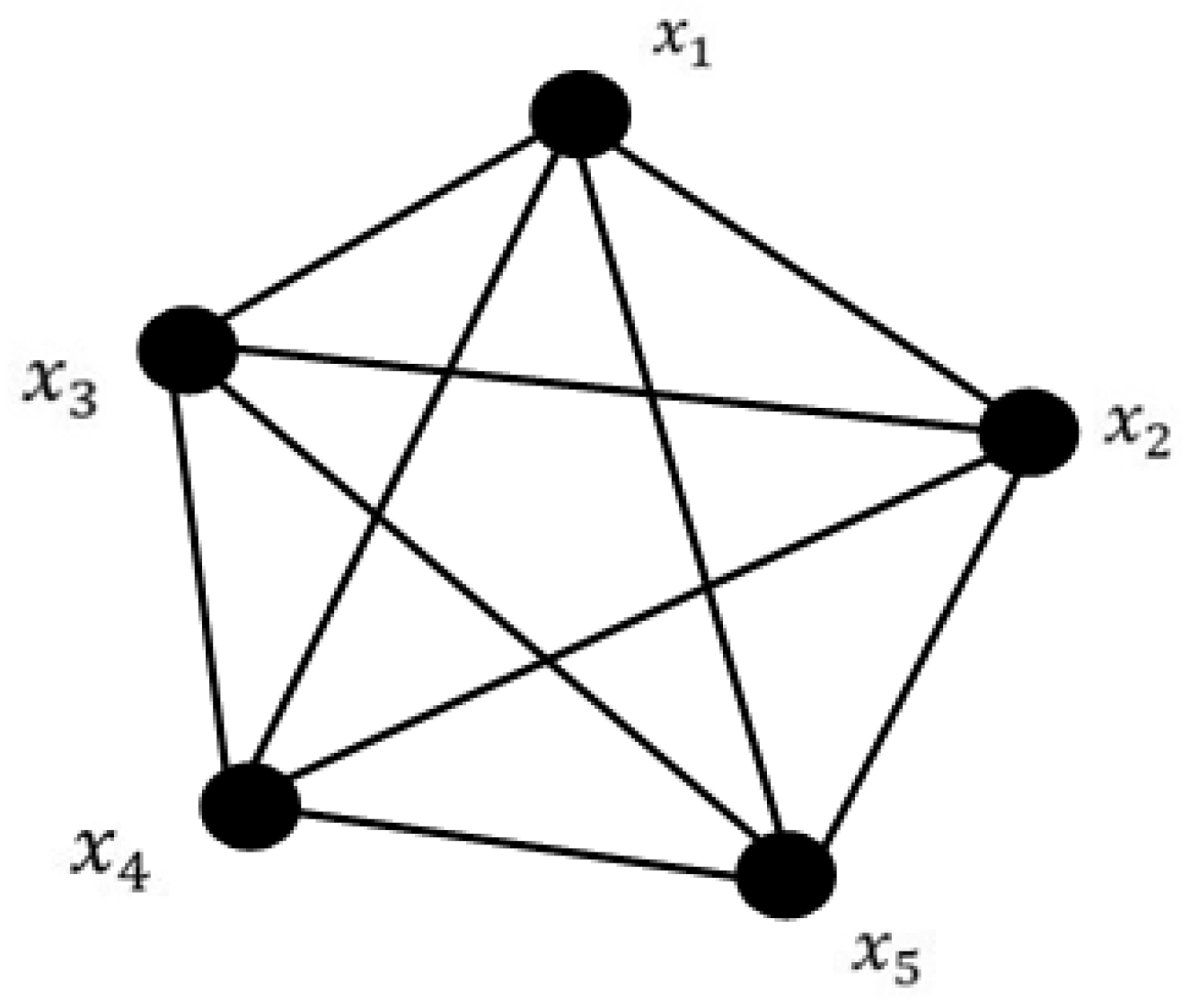
DE uses different population size values to solve a single problem, chosen by trial and error method [21]. Furthermore, in certain studies, varying population sizes are occasionally selected for individual problems under consideration [22]. In differential evolution, the single population approach uses a single population and executes the operations on a single population with different dimensions sizes [23]. In a single population approach, the concept of a panmictic population is used. The population is given by $\{x_1,x_2,x_3,x_4,x_5\}$, as shown in Figure 1.

3.1.1. Classical Differential Evolution

The classical DE algorithm implements a different parameter setting population, and newly generated solutions at the current time are included in the population. They can interact with the current generation and offspring derived from their parental solutions [24,25].

3.1.2. Synchronous Differential Evolution

The synchronous DE algorithm is implemented on classical differential evolution [26]. The classical DE algorithm differs from the synchronous DE algorithm in terms of the latter’s utilization and updating of vector information during the current iteration, while other differential evolution algorithms use an updated population in the next iteration [27].

3.2. Cellular Differential Evolution

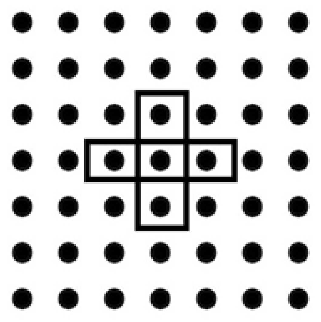
Cellular topology is used in the single-population approach. In this approach, the mutation strategy uses only the vectors of the neighbors. This topology also arranges the population neighbor distance. Figure 2 shows that during selecting the neighbor, it uses the Euclidean distance that is used to reduce the population size during its usage to achieve the high performance of vector the during selection operation and mutation operation [22].

3.3. Multi-Population Approach

Differential evolution uses different approaches to enhance population diversity. In the multi-population approach, this algorithm divides total populations into sub-populations and runs the algorithm in all sub-problems parallel [28]. At the end of the first generation, all results are merged, and the population is updated. For the next generation, the whole population is divided again into sub-populations. The multi-population approach involves dividing the population into a predetermined number of sub-populations [29]. All sub-populations can exchange and share their parameters and individuals during evolution [24]. Mostly, multi-population evolutionary algorithms use the arithmetic mean calculation to migrate the vectors and data in sub-populations, and some algorithms exchange information in the mutation operation. Some algorithms use the best vector from other sub-populations and share the best fitness vectors in population evolution. After the first generation, the population is updated and divided again into sub-populations according to their best fitness. The multi-population algorithm uses the arithmetic mean to find the sub-population fitness through the best fitness exchange information between sub-populations.

3.3.1. Distributed Differential Evolution

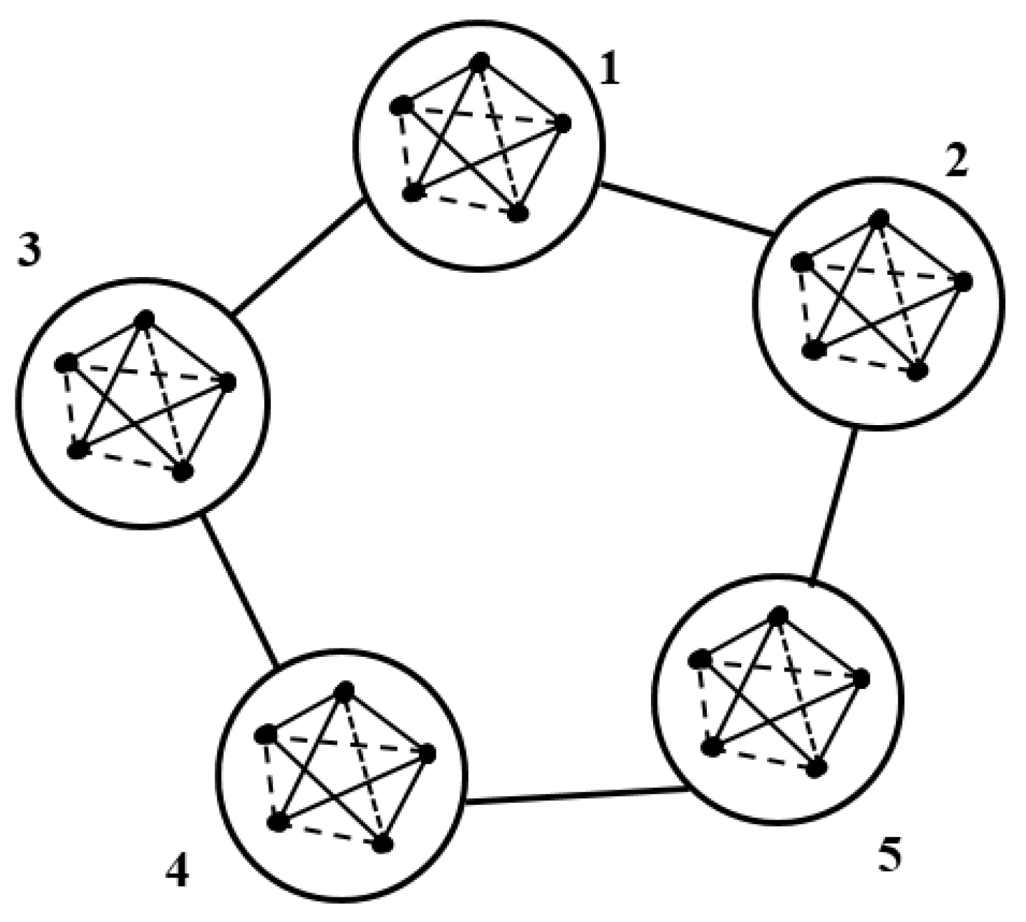
In the distributed differential evolution approach, the population is split into sub-populations, like several islands, that are independent. Islands are the sub-populations in the DE algorithm [22]. All sub-populations are computed separately, and after that, their results are shared. Every island has a model of populations in the distributed DE [30]. Figure 3 illustrates the concept of distributed population.

3.3.2. Heterogeneous Distributed Differential Evolution

Heterogeneous differential evolution also divides the population into sub-populations like distributed differential evolution [31]. In heterogeneous DE, the algorithm uses some more parameters with variations in operations, and this algorithm uses a fixed population size, but in sub-populations, the size varies. Each sub-population gains or loses individuals according to their evolution performance [32]. The algorithm processes sub-populations to find better operations itself so that the overall performance of the algorithm is better.

3.3.3. Hierarchical Cellular Differential Evolution

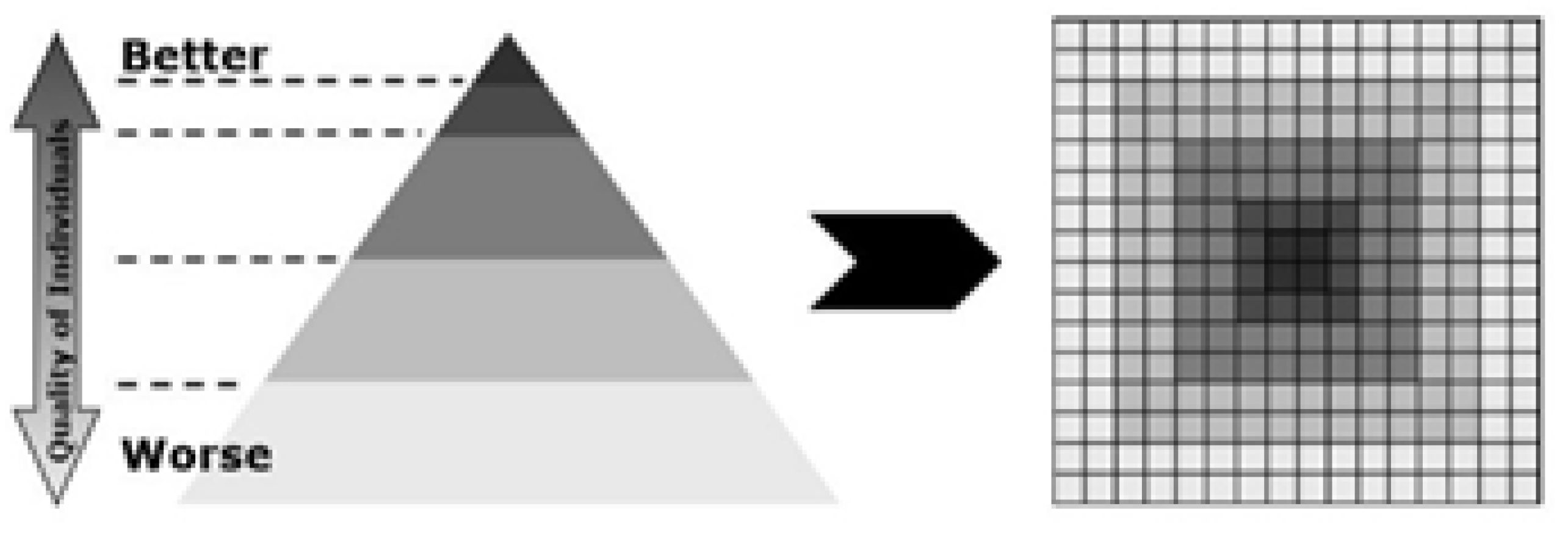
The hierarchical cellular differential evolution algorithm is like cellular topology [33]. It makes the sub-populations of a single population, calculates their fitness, and arranges the sub-populations according to their fitness. Figure 4 shows a display of sub-populations and arranges them, and the good fitness population is in the center. It achieves high performance in searching at the population level. Therefore, by using this approach, the algorithm achieves better solutions in minimal time. To access the other regions that are far from the center, it requires more execution time, and the performance of the algorithm becomes poor. This leads to premature convergence of the population to access other regions far from the center.

3.4. Population Diversity Schemes

The population size in differential evolution must exceed the number of vectors that are used in the algorithm to perform operations. Operations like mutation need three vectors, one of which is the base vector, or else the operations are not completed [34]. Population size has an important impact on the differential evolution algorithm evolutionary process and performance of the algorithm. During the entire population search process, the differential evolution operation may not effectively preserve a high level of population diversity [35]. Differential evolution algorithms use many operations that are used to find fitness, the distance between individuals, and search operations. Population diversity increases the performance of algorithm operation to find the distance between individuals, and their fitness and partitioned the population in sub-populations, but it cannot prove to find the probability of sub-populations without adding some extra terms [36].

3.4.1. Customized Population Sizing for Individual Problems

In the differential evolution algorithm, Storn and Price utilized distinct values for individuals for each specific problem they encountered and determined the population size through trial and error. In many other problems after that, studies used different fixed population sizes in many different problems [11]. It requires more research to find better solutions because this approach does not satisfy the users to select the fixed size according to their selected algorithm and selecting the best point and tuning of population size is not better.

3.4.2. Dimension-Dependent Population Sizing

The DE algorithm has a number of operations that depend on the size of the population [37]. This approach is related to problem dimensionality, d, and population size. Stron and Price recommended setting the population size within a specific range, between 5 times the dimensionality, $5d$, and 10 times the dimensionality, $10d$, and claimed the choice of that is three control parameters that are difficult to use [38]. The hint to use population sizes equal to $10d$ is applied to and used in many differential algorithms [11]. Sometimes, a population size equal to $5d$ is also used [39]. Price [40] states that population sizes as large as $20d$ should be suggested. In the DE, the usage of a large population size puts a burden on the speed of the algorithm and the best population size varies according to algorithms from $2d$ to $40d$, and this depends on the problem. Many studies on population size show the impact on the differential evolution algorithm performance that should not be fixed and suggest that the varying population size should be between $3d$ and $8d$. However, experimental results and population sizes are dependent on problem properties and on the values of control parameters. Some research papers suggest that small population sizes can also be used, e.g., $1d$.

3.4.3. Problem of Dimensionality-Independent Population Size

The impact of the performance of the differential evolution algorithm depends on the problem dimensionality and population size [6]. This approach uses the dimensionality that is independent of population size that uses the fixed population size and dimensions size is independent. Conversely, if dimension size is fixed, then population size is independent. The study of [41] uses a fixed population size of 50–100 individuals, and dimension sizes are independent in the micro-DE algorithm, which uses a small population size that gives the best results and sets the population size as low as 5 [11]. In [39], a fixed population size between 10 and 80 and between 200 and 250 is used. The AEPD algorithm [42] uses many population size problems, an independent dimension size is used, and it is found that the best population size is 30.

4. Proposed Approach

4.1. Variable Population Size

In differential evolution, it is common practice to maintain a fixed population size, but few research studies have suggested using a variable-size population. In the research of [40], two algorithms that use variable population size and self-arrange that population size are proposed. In the adaptive multi-population differential evolution (AMPDE) algorithm [40] and multi-population differential evolution (MPDE) algorithm [40], the population size is set to $10d$. After every generation, the individual levels are self-adapted, and in both approaches, three mutation strategies are used for parents. Very few researchers have focused on variable population sizes. Differential evolution algorithm performance varies depending on the different variants, and it gives better and more efficient results on large population size than the versions of small population size. The diversity of the population is supported by the fact that a large size of the population has diverse members, which leads to high performance due to the ability of the algorithm to obtain a global solution(s) [43].

In past years, research works on differential evolution focused on developing large population size approaches [44]. In a slow computation speed problem, the proposed methodology is first to convert the population into sub-populations and then select the mutation strategy, which is applied only to selected sub-population individuals. Similarly, three mutation strategies are used, which are applied to all sub-populations. A single sub-population uses a single mutation strategy, which is selected randomly. To address the premature population convergence problem, the population is split into sub-populations. After every generation, all sub-populations are merged; then, each population is again converted into sub-populations in the next iteration. If the count of sub-populations is on the rise and the arithmetic mean of the current whole population fitness is better than the arithmetic mean of the previous whole population fitness, then the number of sub-populations is decreased. Conversely, if the arithmetic mean of the current whole population fitness is equal to or less than the arithmetic mean of the previous whole population fitness, then the number of populations is increased.

4.2. Proposed Improved Multi-Population Ensemble Differential Evolution

The proposed improved multi-population ensemble differential evolution (IMPEDE) method enhances the differential evolution algorithm by leveraging the mutation factor’s capability to increase the population’s diversity. Consequently, the population exhibits significantly higher diversity throughout the search process. Multi-population ensemble differential evolution (MPEDE) is used for the improvement in DE population diversity and uses the proposed scheme in that algorithm. The arithmetic mean of fitness is calculated by using the following equation:

$$\Delta f=\frac{{\sum }_{i=0}^n{f}_i}{n}$$

(4)

In the proposed scheme, $pn$ is used for a number of total sub-populations that are increased according to the arithmetic mean of all population fitness.

$$\left\{\begin{array}{cc}pn=pn+1,\hfill & \mathit{if}\Delta f_j<\Delta f_{j-1}\hfill \\ pn=pn-1,\hfill & otherwise\hfill \end{array}\right.$$

(5)

Figure 5 shows the workflow of the proposed approach. The working of each sub-module is discussed subsequently.

For performance comparison, six fitness functions are used in the MPEDE, DE, HDDE, and IMPEDE algorithms to compare the results of all algorithms. The proposed algorithm IMPEDE uses a new functionality that controls the number of sub-populations in every generation and counts the arithmetic mean of all population fitness. It uses three mutation functions that are selected randomly like previous algorithms. The execution of IMPEDE is explained in Algorithm 3.

DE starts with randomly generated populations, $NP$, of feasible solutions, $P_G=$$\{X_{1,G},X_{2,G},\dots ,X_{NP,G}\}$. Population objects are called individuals, and single individuals are $X_{i,G}=x_{i,G}^1,x_{i,G}^2,\dots ,x_{i,G}^D,i=1,2,\dots ,NP$. G denotes the number of generations that are used to increase the algorithm calls, and D is the number of dimensions for a single individual. For individuals, each dimension is displayed randomly in the range [$X_{min},X_{max}$], where $X_{min}=x_{min}^1,x_{min}^2,\dots ,x_{min}^D$ and $X_{max}=x_{max}^1,x_{max}^2,\dots ,x_{max}^D$.

Then, mutation, crossover, and selection operations are used. For the next generation, the number of sub-populations is increased according to the total population average. If the fitness of the next population is increased, then the number of sub-populations is increased; otherwise, the number of sub-populations is decreased.

Algorithm 3 IMPEDE algorithm.

Start parameter initializing: F is scaling factor, N is population size, $C_r$ is crossover rate Set population vector $\{X_{1,G},X_{2,G},\dots ,X_{NP,G}\}$ Total sub-population numbers $pn$. First time selected $pn=4$ Set iteration/generation counter $G\leftarrow 0$ Calculate $\Delta f_j$ while  $G\le maxG$  do    Now, randomly divide population into sub-populations $1,2,3,\dots ,pn$ according to their size.    Merge the last sub-population with randomly selected other sub-populations as a reward and adjust the size of that population. Let $P_j$ = $P_j$ U $pn$ and $N{P}_j=N{P}_j$ U $N{P}_{pn}$;    for $j=1\to pn$ do      for all  $i\in \{1,2,\dots ,Np\}$ do       $V_{i,G}\leftarrow$differential mutation$(F;x_{1,G},\dots ,x_{NP,G})$       $U_{i,G}\leftarrow crossover(C_r;X_{i,G},V_{i,G}$       Calculate fitness for fitness functions $f1,...,f6$       if $f\left(X_{i,G}\right)\le f\left(U_{i,G}\right)$ then        $X_{i,G+1}=U_{i,G}$       else        $X_{i,G+1}=X_{i,G}$       end if     end for    end for    Calculate $\Delta f_{j+1}$    if $\Delta f_{j+1}\le \Delta f_{j+1}$ then     $pn=pn+1$    else     $pn=pn-1$    end if        Merge all sub-populations $1,2,3,4\dots ,pn$ end while return  $argma{x}_{X_{i,G}}f\left(X_{i,G}\right)$

5. Results and Discussions

5.1. Parameter Settings and Simulation Results

In the proposed algorithm, IMPEDE, we have used many functions to generate the results with the base algorithm. Three distinct mutation strategies are employed to generate the mutant vector. The parameter we have used for IMPEDE is the same as in the DE algorithm, except for the population. We use $F=0.8$, $Cr=0.2$, and $-5\le P_{NP}\le +5$. Population sizes of 100 NP, 150 NP, and 200 NP are used, while dimension sizes of 10D, 30D, and 50D are used for mutation.

The mutation operation creates a mutant vector by using other vectors, which are selected randomly. Different vectors are selected using different techniques. For the proposed algorithm, IMPEDE, amplification factor, F, is used, while the constant, K, is used as $0<K<1$. The following mutation strategies are used in IMPEDE:

$$V_{i,G}=X_{x,G}+F\ast \left(X_{y,G}-X_{z,G}\right),x\ne y\ne z\ne i$$

(6)

$$V_{j,G}=X_{j,G}+K\ast \left(X_{x,G}-X_{j,G}\right)+F\ast \left(X_{y,G}-X_{z,G}\right),x\ne y\ne z\ne j$$

(7)

$$V_{j,G}=X_{j,G}+F\ast \left(X_{best,G}-X_{j,G}+X_{y,G}-X_{z,G}\right),y\ne z\ne j$$

(8)

The above three mutation strategies are used in the algorithm, which are selected randomly, and each sub-population is processed.

$$\sum _{i=0}^{pn}s{p}_i=1$$

(9)

Let $pn$ be the number of total sub-populations, and every sub-population, $s{p}_1,s{p}_2,s{p}_3,\dots ,$$s{p}_{pn}$, uses a mutation strategy randomly. The crossover operation is used to generate a trail vector by using a target vector and a mutant vector. Binomial crossover is used in IMPEDE for the crossover operation.

$$U_{k,G}=\left\{\begin{array}{cc}{V}_{k,G},\hfill & \mathit{if}ran{d}_j(0,1)\le C_{r}orj=j_{rand}\hfill \\ X_{k,G},\hfill & otherwise\hfill \end{array}\right.$$

(10)

The selection operation is a greedy operation that is used to select the best vector between the target vector and the trail vector. IMPEDE uses a selection operation to select the best vector between offspring and the selected vector, and the vector having the best fitness is selected for the next generation. The selection function is as follows:

$$X_{j,G+1}=\left\{\begin{array}{cc}{U}_{j,G}\hfill & \mathit{if}f\left(U_{j,G}\right)\le f\left(X_{j,G}\right)\hfill \\ X_{j,G}\hfill & otherwise\hfill \end{array}\right.$$

(11)

where $j=1,\dots ,NP$.

After performing the selection operation, the vector calculates the arithmetic mean of current population fitness and previous population fitness. After calculating fitness, if the newly generated population exhibits the best fitness, it is advisable to increase the number of sub-populations. However, in the absence of improved fitness, it may be more suitable to decrease the number of sub-populations.

5.2. Experimental Results

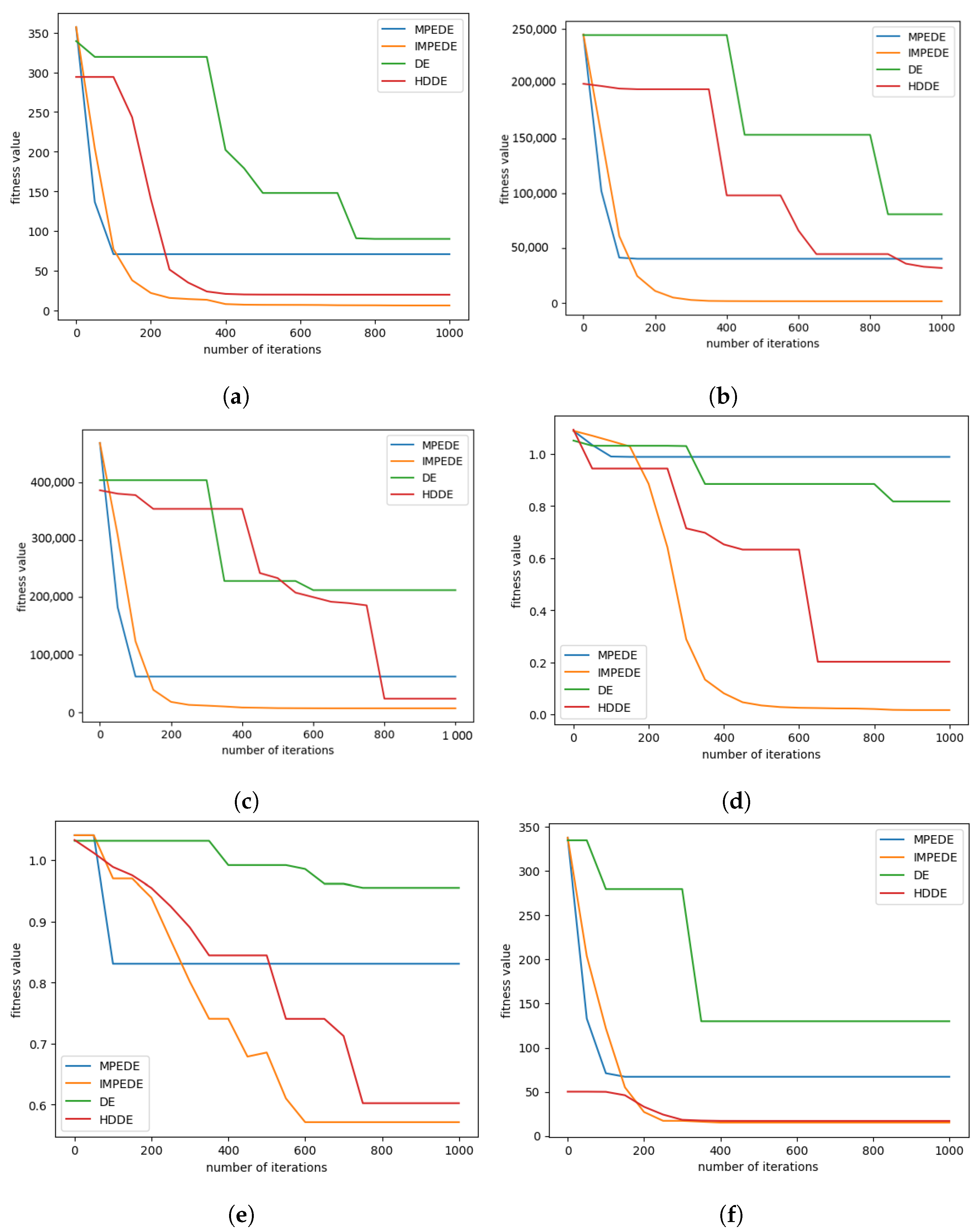
The proposed algorithm, IMPEDE, is implemented along with other DE variants for performance comparison. For this purpose, this study considers MPEDE, DE, and HDDE. IMPEDE is implemented using specified parameter settings. Different combinations of mutations are used to generate the simulated results, and the experiments are performed using 1000, 3000, and 5000 iterations. Figure 6 shows the convergence graphs of all algorithms using 150 NP and 50D. It indicates that the performance of the proposed algorithm, IMPEDE, is better than other algorithms, with a better fitness value, except for Figure 6f, where the fitness values of HDDE and the proposed IMPEDE look very similar.

The results lead to the conclusion that Figure 6 demonstrates the superior performance of IMPEDE in comparison to MPEDE, DE, and HDDE. The evaluation of performance is based on the arithmetic mean ($\mu$) and standard deviation (SDV) of the fitness function value, denoted as f(xbest). The fitness value, f, is obtained from individuals using six benchmark functions. For comparison, different sizes of population and different dimension sizes are used. In fact, the results are considerably improved on benchmark functions $f2$, $f3$, $f4$, and $f5$, and on benchmark functions $f1$ and $f6$, the results are normally improved. The results are compared after 1000 iterations.

Table 1. Comparative results of MPEDE, IMPEDE, DE, and HDDE algorithms with fitness function ($f1$–$f6$) evaluations for 1000 iterations.

Function	Algorithm	Mean (M) and SDV	100 NP			150 NP			200 NP
			10_DIM	20_DIM	30_DIM	10_DIM	20_DIM	30_DIM	10_DIM	20_DIM	30_DIM
$f1$	MPEDE	M	65	248	429	66.5	301	4360	7240	3020	444
		SDV	29.1	87.3	123	40.2	83.7	215	415	778	232
	DE	M	85.1	490	591	79.1	397	5970	9020	4120	602
		SDV	50.9	97.8	291	50.2	97.8	301	507	961	393
	HDDE	M	1.2	07	91	9.1	87	170	53	81	02
		SDV	40.9	281	305	50.1	301	29,600	603	198	307
	IMPEDE	M	37.8	211	369	50.3	223	3910	529	227	402
		SDV	34.1	103	174	38.4	104	17,900	408	111	157
$f2$	MPEDE	M	1600	70,300	342,000	1690	72,000	345,000	1760	70,600	348,000
		SDV	1070	28,100	111,000	1220	26,300	104,000	1110	24,100	90,000
	DE	M	880	79,500	491,000	3010	89,500	501,000	4010	89,600	482,000
		SDV	2090	38,100	212,000	1990	39,100	301,000	2510	31,500	98,700
	HDDE	M	998	7100	1000	910	9100	15,000	870	100	1000
		SDV	987	49,400	272,000	2810	47,500	296,000	2490	47,900	298,000
	IMPEDE	M	878	54,800	286,000	1190	62,900	297,000	1310	58,900	309,000
		SDV	946	30,600	143,000	1090	30,500	136,000	1090	30,200	119,000
$f3$	MPEDE	M	89,200	417,000	735,000	90,400	431,000	755,000	2010	438,000	764,000
		SDV	71,100	189,000	279,000	72,400	203,000	262,000	75,200	178,000	232,000
	DE	M	99,700	569,000	905,000	2010	604,000	903,000	3750	597,000	922,000
		SDV	90,100	348,000	492,000	89,700	349,000	438,000	93,100	299,000	439,000
	HDDE	M	9000	95,000	03000	9000	17,000	1000	9100	2000	51,000
		SDV	79,100	384,000	502,000	70,100	397,000	403,000	89,400	347,000	572,000
	IMPEDE	M	44,900	345,000	576,000	63,000	379,000	685,000	73,800	402,000	696,000
		SDV	60,400	209,000	356,000	64,100	208,000	28,7000	71,800	189,000	313,000
$f4$	MPEDE	M	0.956	1.04	1.2	0.944	1.05	1.11	0.969	1.05	1.11
		SDV	0.183	0.0749	0.0311	0.0223	0.00718	0.00332	0.0151	0.0103	0.0282
	DE	M	0.0341	0.55	0.92	0.0261	0.74	0.79	0.0197	0.91	3.05
		SDV	0.371	0.0891	0.0469	0.0381	0.00891	0.00491	0.0298	0.0291	0.0405
	HDDE	M	0.99	0.897	2.03	0.941	2.71	3.12	1.02	4.09	0.02
		SDV	0.381	0.601	0.583	0.491	0.489	0.507	0.503	0.407	0.401
	IMPEDE	M	0.819	0.742	0.867	0.762	0.92	0.94	0.819	0.96	1.03
		SDV	0.249	0.41	0.411	0.335	0.331	0.375	0.321	0.283	0.265
$f5$	MPEDE	M	1.1	1.18	1.18	1.13	1.18	1.18	1.15	1.17	1.18
		SDV	0.197	0.111	0.0887	0.203	0.106	0.0894	0.209	0.129	0.0766
	DE	M	0.89	3.05	3.01	3.71	2.98	2.9	2.73	2.87	2.82
		SDV	0.315	0.281	0.00279	0.301	0.356	0.0974	0.389	0.291	0.0901
	HDDE	M	0.995	0.85	0.15	0.89	0.79	0.74	0.91	0.02	0.02
		SDV	0.581	0.397	0.371	0.459	0.301	0.414	0.487	0.391	0.341
	IMPEDE	M	0.901	1.05	1.09	1.02	1.12	1.1	1.05	1.11	1.14
		SDV	0.307	0.232	0.191	0.282	0.182	0.213	0.279	0.2	0.151
$f6$	MPEDE	M	67.6	242	419	649	2530	4290	70.1	254	451
		SDV	35.9	90.1	125	3710	809	119	34.2	74.4	99.3
	DE	M	84.9	426	590	825	4360	6090	85.9	427	611
		SDV	50.1	99.7	281	4630	993	302	50.7	90.9	281
	HDDE	M	0.9	58	4.1	19	09	73	3.91	910	610
		SDV	509	283	3710	591	2.98	301	571	30.6	14.8
	IMPEDE	M	46.1	193	36.9	471	329	401	56.1	2230	3930
		SDV	339	111	1850	391	91.9	145	381	996	14.8

shows convergence results of MPEDE, IMPEDE, DE, and HDDE on benchmark functions $f1$ to $f6$ using a population size of 150, a dimension size of 50, and 1000 iterations. Furthermore,

Table 2. Comparative results of MPEDE, IMPEDE, DE, and HDDE algorithms with fitness function ($f1$–$f6$) evaluations for 3000 iterations.

Function	Algorithm	Mean (M) and SDV	100 NP			150 NP			200 NP
			10_DIM	20_DIM	30_DIM	10_DIM	20_DIM	30_DIM	10_DIM	20_DIM	30_DIM
$f1$	MPEDE	M	65	251	429	65.9	255	4370	7120	2710	4440
		SDV	33.9	87.3	123	36	84.1	12.9	349	778	11.2
	DE	M	80.2	380	593	81.1	401	6150	8870	4610	6260
		SDV	40.5	99.3	281	50.9	99.1	32.2	511	977	36.5
	HDDE	M	50.4	395	506	68.8	449	53.8	6960	3810	573
		SDV	49.1	279	314	54.8	269	3110	581	26.4	390
	IMPEDE	M	38.2	211	387	4.98	219	38.3	5410	2190	402
		SDV	33.9	103	174	38.4	104	1770	407	10.8	149
$f2$	MPEDE	M	1590	69,100	351,000	1690	71,500	343,000	1760	70,600	351,000
		SDV	993	28,100	112,000	1170	26,300	107,000	1200	24,100	90,000
	DE	M	299	78,800	502,000	2970	87,400	502,000	3050	90,100	491,000
		SDV	3010	34,100	294,000	3710	40,600	291,000	2530	40,300	98,200
	HDDE	M	964	67,100	452,000	3160	78,300	411,000	4020	75,100	490,000
		SDV	991	48,700	307,000	2710	49,100	301,000	2910	48,100	301,000
	IMPEDE	M	878	54,800	289,000	1200	63,100	297,000	1280	58,900	309,000
		SDV	946	30600	143,000	1090	30,500	136,000	1120	30,200	124,000
$f3$	MPEDE	M	89,200	417,000	741,000	90,400	431,000	755,000	99,400	441,000	759,000
		SDV	70,900	189,000	279,000	72,400	182,000	262,000	75,200	178,000	241,000
	DE	M	2010	59,900	871,000	3120	607,000	901,000	3010	604,000	925,000
		SDV	87,100	307,000	415,000	93,100	322,000	409,000	90,100	361,000	401,000
	HDDE	M	62,100	503,000	622,000	80,100	519,000	801,000	90,400	591,000	831,000
		SDV	78,100	369,000	495,000	80,200	382,000	438,000	88,100	341,000	491,000
	IMPEDE	M	45,000	339,000	576,000	62,900	382,000	685,000	72,900	39,800	696,000
		SDV	60,600	213,000	356,000	64,100	211,000	287,000	71,900	193,000	313,000
$f4$	MPEDE	M	0.956	1.05	1.11	0.0944	1.12	12.1	0.0974	10.6	11.2
		SDV	0.191	0.0749	0.0311	0.00214	0.0731	0.339	0.00151	0.0103	0.00283
	DE	M	2.01	3.02	2.92	0.301	2.11	29.4	0.201	28.1	29.8
		SDV	0.302	0.0932	0.0492	0.00375	0.0901	0.473	0.00292	0.0275	0.00401
	HDDE	M	0.981	0.913	0.981	0.903	0.998	2.03	0.971	0.998	2.76
		SDV	0.401	0.571	0.594	0.484	0.501	0.491	0.495	0.342	0.401
	IMPEDE	M	0.819	0.739	0.867	0.758	0.92	0.94	0.817	0.957	1.03
		SDV	0.258	0.41	0.409	0.335	0.318	0.369	0.321	0.283	0.267
$f5$	MPEDE	M	1.1	1.22	1.18	1.15	1.18	1.18	1.13	1.23	1.18
		SDV	0.205	0.108	0.0887	0.192	0.106	0.0894	0.222	0.129	0.0771
	DE	M	2.91	2.82	2.91	2.99	3.09	2.69	2.91	3.01	2.68
		SDV	0.387	0.281	0.0969	0.351	0.291	0.0879	0.394	0.281	0.0941
	HDDE	M	0.981	2.79	2.61	2.81	3.01	2.69	2.71	2.97	2.69
		SDV	0.491	0.401	0.371	0.467	0.374	0.395	0.471	0.396	0.307
	IMPEDE	M	0.884	1.05	1.07	1.01	1.09	1.11	1.04	1.11	1.14
		SDV	0.307	0.232	0.189	0.282	0.184	0.212	0.286	0.2	0.142
$f6$	MPEDE	M	68.1	242	419	6610	2540	43.9	69.9	254	437
		SDV	35.9	90.1	122	369	809	1290	35.1	74.4	105
	DE	M	85.1	401	584	8410	4230	58.6	88.1	422	612
		SDV	50.3	99.8	279	515	963	3790	52.2	91.9	274
	HDDE	M	60.3	3460	5030	6040	401	564	7480	403	574
		SDV	512	35.9	30.1	561	3.01	3290	548	20.1	327
	IMPEDE	M	46.1	1820	3630	4710	229	398	5530	223	392
		SDV	329	12.2	17.5	384	91.8	1460	368	995	142

shows the convergence results of MPEDE, IMPEDE, DE, and HDDE algorithms on fitness functions $f1$ to $f6$ using a population size of 150, a dimension size of 50, and 3000 iterations. In early iterations, the results are similar, but as the number of iterations increases, IMPEDE results are more improved than MPEDE, DE, and HDDE.

The number of training iterations in the convergence graphs are reported horizontally and average fitness values are shown vertically. It can be observed from these sub-figures that convergence performance of proposed algorithm and three other state of the art algorithms is similar in the starting iterations but as the number of iterations starts increasing, the performance of proposed algorithm starts minimizing quickly and it is continuously minimizing till the last iteration. It can be summarized that the convergence speed of the proposed algorithm in minimizing the problems is better than DE algorithm, MPEDE algorithm and HODE algorithm

It can be summarized from the results that IMPEDE’s performance is better, as compared to MPEDE, DE, and HDDE in

Table 3. Comparative results of MPEDE, IMPEDE, DE, and HDDE algorithms with fitness function ($f1$–$f6$) evaluations for 5000 iterations.

Function	Algorithm	Mean (M) and SDV	100 NP			150 NP			200 NP
			10_DIM	20_DIM	30_DIM	10_DIM	20_DIM	30_DIM	10_DIM	20_DIM	30_DIM
$f1$	MPEDE	M	65	248	429	66.5	255	43.7	7120	2580	4450
		SDV	33.9	87.3	123	36	83.7	1180	354	778	10.3
	DE	M	81.6	391	584	80.1	414	58.4	8740	4010	5940
		SDV	48.1	99.5	301	51.3	97.1	2950	501	915	28.4
	HDDE	M	51.2	371	501	68.5	387	5640	6860	379	569
		SDV	48.3	278	315	50.7	291	30.9	583	259	381
	IMPEDE	M	37.8	211	387	50.3	219	3830	5290	227	402
		SDV	33.9	103	174	38.4	104	17.7	419	107	157
$f2$	MPEDE	M	1590	68,300	342,000	1690	71,500	343,000	1760	70,600	348,000
		SDV	1040	27,900	108,000	1170	26,300	104,000	1110	24,100	90,000
	DE	M	3010	81,500	509,000	2910	88,400	501,000	3080	89100	479,000
		SDV	2350	40,100	291,000	2690	40,100	298,000	2870	40,900	2010
	HDDE	M	981	70,100	452,000	2950	80,300	461,000	2930	74,300	494,000
		SDV	20.1	49,700	284,000	2790	44,900	281,000	2590	49,100	284,000
	IMPEDE	M	878	54,800	289,000	1200	62,900	297,000	1280	58,900	311,000
		SDV	946	30,600	143,000	1090	30,500	136,000	1120	30,200	124,000
$f3$	MPEDE	M	89,200	417,000	735,000	90,400	431,000	755,000	99,400	438,000	764,000
		SDV	71,100	189,000	279,000	72,400	182,000	262,000	75,200	178,000	232,000
	DE	M	98,600	569,000	875,000	2140	591,000	901,000	3090	579,000	901,000
		SDV	87,900	340,000	408,000	89,700	353,000	407,000	90,400	349,000	407,000
	HDDE	M	59,100	501,000	704,000	81,500	539,000	873,000	91,900	579,000	848,000
		SDV	76,900	379,000	504,000	79,400	360,000	409,000	86,900	348,000	473,000
	IMPEDE	M	45,000	345,000	576,000	63,000	382,000	685,000	73,800	402,000	696,000
		SDV	60,600	213,000	356,000	64,100	211,000	287,000	72,100	193,000	313,000
$f4$	MPEDE	M	0.956	1.05	1.11	0.944	1.05	1.11	0.00973	10.6	11.2
		SDV	0.183	0.0749	0.0311	0.213	0.0719	0.0331	0.0147	0.0103	0.00283
	DE	M	2.04	2.91	2.83	3.02	2.81	2.94	0.0301	27.1	29.3
		SDV	0.351	0.0904	0.0493	0.384	0.0869	0.048	0.0301	0.0274	0.00428
	HDDE	M	0.979	0.951	0.973	0.98	2.05	3.15	0.994	1.91	2.85
		SDV	0.402	0.593	0.604	0.517	0.531	0.493	0.496	0.451	0.405
	IMPEDE	M	0.819	0.742	0.867	0.762	0.92	0.94	0.817	0.96	1.03
		SDV	0.258	0.41	0.412	0.335	0.329	0.375	0.321	0.283	0.267
$f5$	MPEDE	M	1.1	1.18	1.18	1.13	1.18	1.18	1.13	1.17	1.18
		SDV	0.205	0.108	0.0887	0.192	0.106	0.0894	0.213	0.129	0.0766
	DE	M	2.81	2.94	3.01	2.79	2.84	2.71	2.65	2.91	2.83
		SDV	0.349	0.273	0.201	0.374	0.257	0.258	0.394	0.281	0.0954
	HDDE	M	0.997	2.71	2.64	2.85	2.87	2.91	2.75	2.55	2.79
		SDV	0.415	0.371	0.348	0.464	0.317	0.396	0.417	0.377	0.379
	IMPEDE	M	0.884	1.05	1.09	1.02	1.12	1.1	1.05	1.11	1.14
		SDV	0.307	0.232	0.189	0.282	0.184	0.213	0.286	0.2	0.142
$f6$	MPEDE	M	67.7	242	419	6490	2540	4290	69.9	254	434
		SDV	35.9	89.5	118	371	809	119	34.2	74.4	105
	DE	M	81.8	391	569	7810	4170	5800	85.8	391	584
		SDV	50.4	2.17	257	524	971	284	49.5	88.1	261
	HDDE	M	59.1	358	5010	6380	385	564	693	379	509
		SDV	5.09	258	29.7	565	2.01	2970	5070	305	281
	IMPEDE	M	45.8	193	3580	4710	232	398	553	223	392
		SDV	3.45	107	17.5	384	92.4	1460	3680	9950	138

. To evaluate the performance, the arithmetic mean ($\mu$) and the standard deviation (SDV) of the fitness function value f(xbest) are employed. Here, f represents the fitness value of each individual, which is determined using six benchmark functions. In comparison, different population sizes and different dimension sizes are used. The results given in Table 1, Table 2 and Table 3 prove that the proposed algorithm IMPEDE produces much better results for benchmark functions $f1$, $f2$, $f3$, and $f4$, while the results for benchmark functions $f5$ and $f6$ are marginally improved.

5.3. Discussion

DE is a straightforward yet highly efficient search technique renowned as one of the top evolutionary algorithms employed for solving practical challenges in the real world. In DE, the concept of multiple populations is attractive, and this study has adopted this concept to produce better results. The proposed IMPEDE uses different parameters for execution that convert the whole population into many sub-populations that enhance the population diversity and performance.

In the proposed scheme, the number of sub-populations is increased or decreased according to the performance of the algorithm. The DE algorithm with different variants shows better and more efficient results on small population sizes compared to large population sizes. The diversity of the population is supported by the large size of the population, where members are diverse, which is helpful in achieving high performance by achieving the global optimum. In the past years, research works on DE focused on developing approaches for large population sizes. Previous research works use the static strategy of creating a number of sub-populations, but the proposed method uses a dynamic strategy of creating sub-populations. The number of sub-populations can be adjusted, either increased or decreased, based on the performance.

Six fitness functions are used to analyze the performance of the proposed algorithm in comparison to DE, HDDE, and MPEDE. Experimental analysis shows that the IMPEDE algorithm, which uses sub-populations and increases or decreases the number of sub-populations, achieves better results than MPEDE, DE, and HDDE algorithms. The performance of the proposed algorithm is compared to MPEDE, DE, and HDDE by using six benchmark functions and using different sizes of populations. Similarly, different dimension sizes are used, and the results are compared after 1000 iterations, 3000 iterations, and 5000 iterations. It is suggested to use the concept of memory for the selection of mutation strategies instead of random selection. Memory can be beneficial for enhancing the performance of IMPEDE.

5.4. Statistical Significance

A statistical significance test is performed with the Friedman significance test for four algorithms using the results of six benchmark functions. The null hypothesis ($H_0$) defines that there is no significant difference in the performance of DE, MPEDE, HDDE, and IMPEDE for benchmark functions $f_1$ to $f_6$. On the other hand, the alternate hypothesis ($H_a$) defines that there is a significant difference in the performance of DE, MPEDE, HDDE, and IMPEDE for benchmark functions $f_1$ to $f_6$. The test statistic in the Friedman significance test is calculated using Equation (12):

$$ts=\frac{12}{rc(c+1)}\ast \sum _{j=1}^c{R_j}^2-3r(c+1)$$

(12)

where $ts$ is test statistic, r is the number of functions used in this study, c is the number of algorithms, and R is the average rank.

We have used a 0.05 level of significance to generate the test statistic and p-value by using the Friedman significance test by considering four algorithms and six benchmark functions. The significance results of the Friedman test are reported in

Table 4. Statistical significance Friedman test of DE, HDDE, MPEDE, and IMPEDE algorithms using 0.05 level of significance.

Population Size	Dimension	Test Statistic	p-Value
100 NP	10D	17	0.000707
	20D	17	0.000707
	30D	10.6	0.014098
150 NP	10D	9.6	0.022291
	20D	15.8	0.001246
	30D	10.8	0.012858
200 NP	10D	4.6	0.203542
	20D	15.65	0.001338
	30D	15	0.001817

by using varying dimension sizes of 10, 20, and 30, and population sizes of 100, 150, and 200, while 5000 training iterations are used for all four algorithms. It can be observed from Table 4 that the p-value, in almost all cases, is less than the level of significance, which implies that the null hypothesis ($H_0$) is rejected. It can be concluded that there is a significant difference in the performance of the proposed algorithm and the three other algorithms used in this study.

6. Conclusions

This study proposes IMPEDE, a differential evolution algorithm that converts the whole population into many sub-populations to enhance the population diversity to obtain a higher performance. The concept of sub-population is preferred due to its high diversity, which is suitable to obtain a global optima. However, contrary to existing works that use a static strategy, in the proposed scheme, the number of sub-populations is adjusted dynamically with respect to the performance of each generation. Experiments are performed using different population sizes, dimension sizes, and a different number of iterations to analyze the efficacy of the proposed IMPEDE in comparison to the existing DE, MPEDE, and HDDE. The experimental results reveal that the IMPEDE algorithm gives better results than the MPEDE, DE, and HDDE algorithms. Using six benchmark functions, $f1$ to $f6$, the proposed algorithm shows substantially better results for $f2$, $f3$, $f4$, and $f5$ while showing marginally better results for $f1$ and $f6$ compared to MPEDE, DE, and HDDE for 1000 iterations, 3000 iterations, and 5000 iterations. The Friedman significance test shows that the proposed algorithm and the other three algorithms’ performance varies significantly at a 0.05 level of significance for the considered benchmark functions. The non-parametric significance Friedman test confirms that there is a significant difference in the performance of the proposed algorithm and the other used algorithms by considering a 0.05 level of significance using six benchmark functions. The results also indicate that the use of memory for selecting mutation strategies can be beneficial over random selection.

References

- Arunachalam, V. Optimization Using Differential Evolution; The University of Western Ontario: London, ON, Canada, 2008. [Google Scholar]
- Zhan, Z.H.; Shi, L.; Tan, K.C.; Zhang, J. A survey on evolutionary computation for complex continuous optimization. Artif. Intell. Rev. 2022, 55, 59–110. [Google Scholar] [CrossRef]
- Liang, J.; Ban, X.; Yu, K.; Qu, B.; Qiao, K.; Yue, C.; Chen, K.; Tan, K.C. A survey on evolutionary constrained multiobjective optimization. IEEE Trans. Evol. Comput. 2022, 27, 201–221. [Google Scholar] [CrossRef]
- Storn, R.; Price, K. Differential evolution—A simple and efficient heuristic for global optimization over continuous spaces. J. Glob. Optim. 1997, 11, 341–359. [Google Scholar] [CrossRef]
- Pan, J.S.; Liu, N.; Chu, S.C. A hybrid differential evolution algorithm and its application in unmanned combat aerial vehicle path planning. IEEE Access 2020, 8, 17691–17712. [Google Scholar] [CrossRef]
- Dixit, A.; Mani, A.; Bansal, R. An adaptive mutation strategy for differential evolution algorithm based on particle swarm optimization. Evol. Intell. 2022, 15, 1571–1585. [Google Scholar] [CrossRef]
- Deng, W.; Shang, S.; Cai, X.; Zhao, H.; Song, Y.; Xu, J. An improved differential evolution algorithm and its application in optimization problem. Soft Comput. 2021, 25, 5277–5298. [Google Scholar] [CrossRef]
- Abbas, Q.; Ahmad, J.; Jabeen, H. The analysis, identification and measures to remove inconsistencies from differential evolution mutation variants. ScienceAsia 2017, 43S, 52–68. [Google Scholar] [CrossRef]
- Sun, G.; Li, C.; Deng, L. An adaptive regeneration framework based on search space adjustment for differential evolution. Neural Comput. Appl. 2021, 33, 9503–9519. [Google Scholar] [CrossRef]
- Achom, A.; Das, R.; Pakray, P.; Saha, S. Classification of microarray gene expression data using weighted grey wolf optimizer based fuzzy clustering. In Proceedings of the TENCON 2019-2019 IEEE Region 10 Conference (TENCON), Kochi, India, 17–20 October 2019; pp. 2705–2710. [Google Scholar]
- Yang, M.; Li, C.; Cai, Z.; Guan, J. Differential evolution with auto-enhanced population diversity. IEEE Trans. Cybern. 2014, 45, 302–315. [Google Scholar] [CrossRef] [PubMed]
- Zhang, X.; Jin, L.; Cui, C.; Sun, J. A self-adaptive multi-objective dynamic differential evolution algorithm and its application in chemical engineering. Appl. Soft Comput. 2021, 106, 107317. [Google Scholar] [CrossRef]
- Chen, X.; Shen, A. Self-adaptive differential evolution with Gaussian–Cauchy mutation for large-scale CHP economic dispatch problem. Neural Comput. Appl. 2022, 34, 11769–11787. [Google Scholar] [CrossRef]
- Yang, Y.; Forsythe, E.S.; Ding, Y.M.; Zhang, D.Y.; Bai, W.N. Genomic Analysis of Plastid–Nuclear Interactions and Differential Evolution Rates in Coevolved Genes across Juglandaceae Species. Genome Biol. Evol. 2023, 15, evad145. [Google Scholar] [CrossRef] [PubMed]
- Houssein, E.H.; Mahdy, M.A.; Eldin, M.G.; Shebl, D.; Mohamed, W.M.; Abdel-Aty, M. Optimizing quantum cloning circuit parameters based on adaptive guided differential evolution algorithm. J. Adv. Res. 2021, 29, 147–157. [Google Scholar] [CrossRef] [PubMed]
- Lu, K.D.; Wu, Z.G.; Huang, T. Differential evolution-based three stage dynamic cyber-attack of cyber-physical power systems. IEEE/ASME Trans. Mechatron. 2022, 28, 1137–1148. [Google Scholar] [CrossRef]
- Belciug, S. Learning deep neural networks’ architectures using differential evolution. Case study: Medical imaging processing. Comput. Biol. Med. 2022, 146, 105623. [Google Scholar] [CrossRef]
- Abbas, Q.; Malik, K.M.; Saudagar, A.K.J.; Khan, M.B.; Hasanat, M.H.A.; AlTameem, A.; AlKhathami, M. Convergence Track Based Adaptive Differential Evolution Algorithm (CTbADE). CMC-Comput. Mater. Contin. 2022, 72, 1229–1250. [Google Scholar] [CrossRef]
- Zeng, Z.; Hong, Z.; Zhang, H.; Zhang, M.; Chen, C. Improving differential evolution using a best discarded vector selection strategy. Inf. Sci. 2022, 609, 353–375. [Google Scholar] [CrossRef]
- Mohamed, A.W.; Hadi, A.A.; Jambi, K.M. Novel mutation strategy for enhancing SHADE and LSHADE algorithms for global numerical optimization. Swarm Evol. Comput. 2019, 50, 100455. [Google Scholar] [CrossRef]
- Gong, W.; Wang, Y.; Cai, Z.; Wang, L. Finding multiple roots of nonlinear equation systems via a repulsion-based adaptive differential evolution. IEEE Trans. Syst. Man Cybern. Syst. 2018, 50, 1499–1513. [Google Scholar] [CrossRef]
- Salehinejad, H.; Rahnamayan, S.; Tizhoosh, H.R. Micro-differential evolution: Diversity enhancement and a comparative study. Appl. Soft Comput. 2017, 52, 812–833. [Google Scholar] [CrossRef]
- Pant, M.; Zaheer, H.; Garcia-Hernandez, L.; Abraham, A. Differential Evolution: A review of more than two decades of research. Eng. Appl. Artif. Intell. 2020, 90, 103479. [Google Scholar]
- Dorronsoro, B.; Bouvry, P. Improving classical and decentralized differential evolution with new mutation operator and population topologies. IEEE Trans. Evol. Comput. 2011, 15, 67–98. [Google Scholar] [CrossRef]
- Eltaeib, T.; Mahmood, A. Differential evolution: A survey and analysis. Appl. Sci. 2018, 8, 1945. [Google Scholar] [CrossRef]
- Choi, T.J.; Lee, Y. Asynchronous differential evolution with selfadaptive parameter control for global numerical optimization. In Proceedings of the 2018 2nd International Conference on Material Engineering and Advanced Manufacturing Technology (MEAMT 2018), Beijing, China, 25–27 May 2018; Volume 189, p. 03020. [Google Scholar]
- Son, N.N.; Van Kien, C.; Anh, H.P.H. Parameters identification of Bouc–Wen hysteresis model for piezoelectric actuators using hybrid adaptive differential evolution and Jaya algorithm. Eng. Appl. Artif. Intell. 2020, 87, 103317. [Google Scholar] [CrossRef]
- Ma, Y.; Bai, Y. A multi-population differential evolution with best-random mutation strategy for large-scale global optimization. Appl. Intell. 2020, 50, 1510–1526. [Google Scholar] [CrossRef]
- Lu, Y.; Ma, Y.; Wang, J. Multi-Population Parallel Wolf Pack Algorithm for Task Assignment of UAV Swarm. Appl. Sci. 2021, 11, 11996. [Google Scholar] [CrossRef]
- Ge, Y.F.; Orlowska, M.; Cao, J.; Wang, H.; Zhang, Y. MDDE: Multitasking distributed differential evolution for privacy-preserving database fragmentation. VLDB J. 2022, 31, 957–975. [Google Scholar] [CrossRef]
- Liu, W.l.; Gong, Y.J.; Chen, W.N.; Zhong, J.; Jean, S.W.; Zhang, J. Heterogeneous Multiobjective Differential Evolution for Electric Vehicle Charging Scheduling. In Proceedings of the 2021 IEEE Symposium Series on Computational Intelligence (SSCI), Orlando, FL, USA, 5–7 December 2021; pp. 1–8. [Google Scholar]
- Yazdani, D.; Cheng, R.; Yazdani, D.; Branke, J.; Jin, Y.; Yao, X. A survey of evolutionary continuous dynamic optimization over two decades—Part A. IEEE Trans. Evol. Comput. 2021, 25, 609–629. [Google Scholar] [CrossRef]
- Zhong, X.; Cheng, P. An elite-guided hierarchical differential evolution algorithm. Appl. Intell. 2021, 51, 4962–4983. [Google Scholar] [CrossRef]
- Zeng, Z.; Zhang, M.; Zhang, H.; Hong, Z. Improved differential evolution algorithm based on the sawtooth-linear population size adaptive method. Inf. Sci. 2022, 608, 1045–1071. [Google Scholar] [CrossRef]
- Gao, S.; Yu, Y.; Wang, Y.; Wang, J.; Cheng, J.; Zhou, M. Chaotic local search-based differential evolution algorithms for optimization. IEEE Trans. Syst. Man Cybern. Syst. 2019, 51, 3954–3967. [Google Scholar] [CrossRef]
- Yu, Y.; Gao, S.; Wang, Y.; Lei, Z.; Cheng, J.; Todo, Y. A multiple diversity-driven brain storm optimization algorithm with adaptive parameters. IEEE Access 2019, 7, 126871–126888. [Google Scholar] [CrossRef]
- Cui, M.; Li, L.; Zhou, M.; Abusorrah, A. Surrogate-assisted autoencoder-embedded evolutionary optimization algorithm to solve high-dimensional expensive problems. IEEE Trans. Evol. Comput. 2021, 26, 676–689. [Google Scholar] [CrossRef]
- Sun, X.; Wang, D.; Kang, H.; Shen, Y.; Chen, Q. A Two-Stage Differential Evolution Algorithm with Mutation Strategy Combination. Symmetry 2021, 13, 2163. [Google Scholar] [CrossRef]
- Opara, K.R.; Arabas, J. Differential Evolution: A survey of theoretical analyses. Swarm Evol. Comput. 2019, 44, 546–558. [Google Scholar] [CrossRef]
- Wu, C.Y.; Tseng, K.Y. Truss structure optimization using adaptive multi-population differential evolution. Struct. Multidiscip. Optim. 2010, 42, 575–590. [Google Scholar] [CrossRef]
- Caraffini, F.; Kononova, A.V.; Corne, D. Infeasibility and structural bias in differential evolution. Inf. Sci. 2019, 496, 161–179. [Google Scholar] [CrossRef]
- Piotrowski, A.P. Review of differential evolution population size. Swarm Evol. Comput. 2017, 32, 1–24. [Google Scholar] [CrossRef]
- Francisco, V.J.; Efren, M.M.; Alexander, G. Empirical analysis of a micro-evolutionary algorithm for numerical optimization. Int. J. Phys. Sci. 2012, 7, 1235–1258. [Google Scholar]
- Rao, R.V.; Saroj, A. A self-adaptive multi-population based Jaya algorithm for engineering optimization. Swarm Evol. Comput. 2017, 37, 1–26. [Google Scholar]