
Counting Polynomials in Chemistry: Past, Present, and Perspectives


Abstract
1. Introduction
2. Characteristic Polynomial
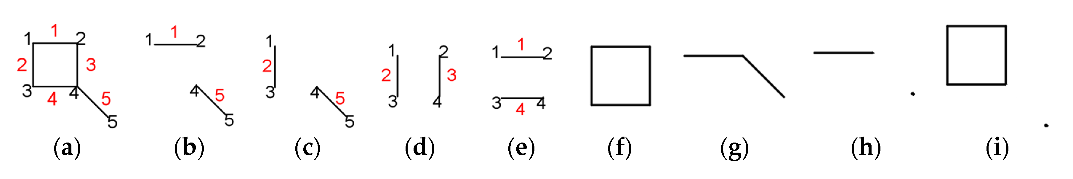
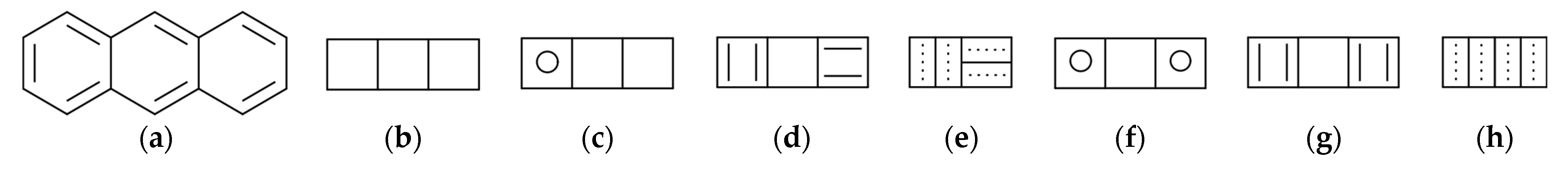
- for k = 0, we count the empty Sachs graph with 0 edges and the result is: ;
- for k = 1, there can be no isolated edge with one vertex nor such a ring, and the result is 0.
- denoting ,
- for k = 0, ;
- for k = 2, since this is the case where each edge represents a Sachs subgraph, ;
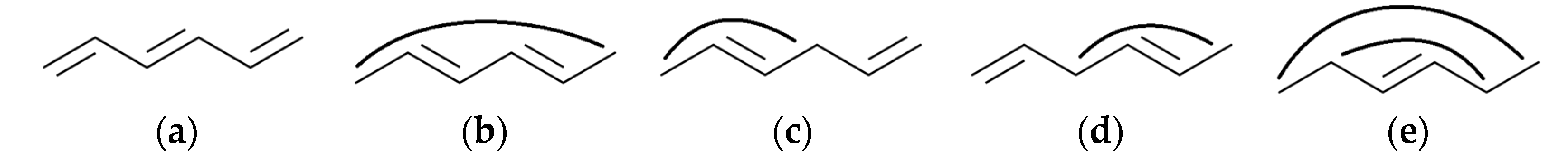
- for k = 3 and k = 5, it can be seen in Figure 1g–i that these are not Sachs subgraphs;
3. Permanental Polynomial
- denoting ,
- for k = 0, ;
- for k = 2, ;
- for k = 3 and k = 5, it can be seen in Figure 1g–i that these are not Sachs subgraphs;
4. Matching Polynomial
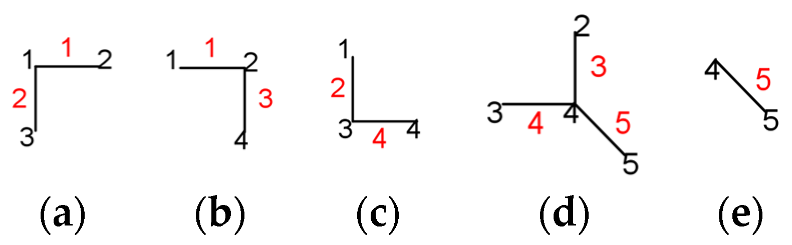
- for k = 0, ni(k) = 1, as there is one possibility of choosing zero edges, namely ∅;
- for k = 1, ni(k) = 5, the number of edges;
5. Hosoya Polynomial
- for k = 0, ni(k) = 1, as there is one possibility of choosing zero edges, namely ∅;
- for k = 1, ni(k) = 5, the number of edges;
6. Immanantal Polynomials
7. Laplacian Polynomial
8. Zagreb Polynomials
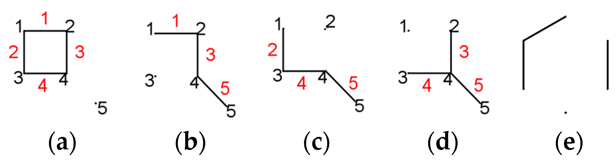
- for k = 1, nu(k) = 2, nv(k) = 2;
- for k = 2, nu(k) = 2, nv(k) = 2;
- for k = 3, nu(k) = 2, nv(k) = 3;
- for k = 4, nu(k) = 2, nv(k) = 3;
- and for k = 5, nu(k) = 3, nv(k) = 1.
9. Sextet Polynomial
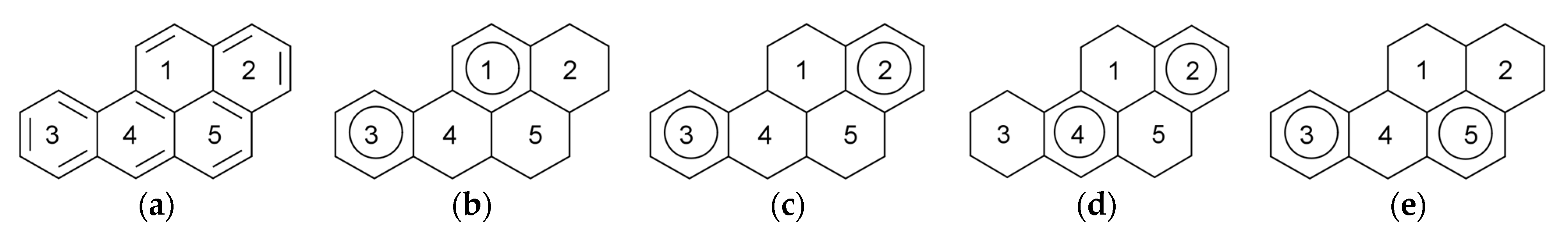
- for k = 0, nr(k) = 1, as there is one possibility of choosing zero sextets, namely ∅;
- for k = 1, nr(k) = 5, the number of benzene rings;
10. Independence Polynomial
- for k = 0, nia(k) = 1, as there is one case of whith zero independent vertices, namely ∅;
- for k = 1, nia(k) = 5, the number of vertices;
- and for k = 2, nia(k) = 5 sets of two independent vertices (1,4; 1,5; 2,3; 2,5; 3,5).
11. King and Domino Polynomials
- for k = 1, nnk(k) = 3, the number of cells;
12. Cluj Polynomial
- for k = 1, nk at = 7, counting how many times “1” appears in our matrix;
- for k = 2, nk at = 6, counting how many times “2” appears in our matrix;
- for k = 3, nk at = 6, counting how many times “3” appears in our matrix;
- for k = 4, nk at = 1, since “4” appears once,
13. Omega Polynomial
- for k = 0, nqoc(k) = 0;
- for k = 1, nqoc(k) = 0;
- for k = 2, nqoc(k) = 4, CO1–4;
- for k = 3, nqoc(k) = 1, CO5.
14. Wheland Polynomial
15. Discussion
Author Contributions
Funding
Data Availability Statement
Conflicts of Interest
References
- Diudea, M.V. Counting Polynomials in Tori T(4,4)S[c, n]. Acta Chim. Slov. 2010, 57, 551–558. [Google Scholar] [PubMed]
- Eliasi, M.; Taeri, B. Extension of the Wiener Index and Wiener Polynomial. Appl. Math. Lett. 2008, 21, 916–921. [Google Scholar] [CrossRef][Green Version]
- Parveen, S.; Awan, N.U.H.; Farooq, F.B.; Hussain, S. Topological Descriptors and QSPR Models of Drugs Used in Blood Cancer. Punjab Univ. J. Math. 2023, 55, 27–43. [Google Scholar] [CrossRef]
- Alviso, D.; Aguerre, H.; Nigro, N.; Artana, G. Prediction of the Physico-Chemical Properties of Vegetable Oils Using Optimal Non-Linear Polynomials. Fuel 2023, 350, 128868. [Google Scholar] [CrossRef]
- Calingaert, G.; Hladky, J.W. A Method of Comparison and Critical Analysis of the Physical Properties of Homologs and Isomers. The Molecular Volume of Alkanes. J. Am. Chem. Soc. 1936, 58, 153–157. [Google Scholar] [CrossRef]
- Kurtz, S.S.; Lipkin, M.R. Molecular Volume of Saturated Hydrocarbons. Ind. Eng. Chem. 1941, 33, 779–786. [Google Scholar] [CrossRef]
- Wiener, H. Structural Determination of Paraffin Boiling Points. J. Am. Chem. Soc. 1947, 69, 17–20. [Google Scholar] [CrossRef]
- Liu, J.-B.; Javed, S.; Javaid, M.; Shabbir, K. Computing First General Zagreb Index of Operations on Graphs. IEEE Access 2019, 7, 47494–47502. [Google Scholar] [CrossRef]
- Bonchev, D.; Rouvray, D.H. (Eds.) Chemical Graph Theory: Introduction and Fundamentals; Mathematical Chemistry; Abacus Press: New York, NY, USA, 1991; ISBN 978-0-85626-454-2. [Google Scholar]
- Dalton, J.; Scattergood, T.; Thorpe, T.E. A New System of Chemical Philosophy; Russell & Allen, Deansgate: Manchester, UK, 1808. [Google Scholar]
- Wollaston, W.H. On Super-Acid and Sub-Acid Salts. Philos. Trans. R. Soc. Lond. B Biol. Sci. 1808, 98, 96–102. [Google Scholar] [CrossRef]
- Kopp, H. Ueber den Zusammenhang zwischen der chemischen Constitution und einigen physikalischen Eigenschaften bei flüssigen Verbindungen. Ann. Chem. Pharm. 1844, 50, 71–144. [Google Scholar] [CrossRef]
- Cayley, F.R.S. LVII. On the Mathematical Theory of Isomers. Lond. Edinb. Dublin Philos. Mag. J. Sci. 1874, 47, 444–447. [Google Scholar] [CrossRef]
- Cayley, E. Ueber Die Analytischen Figuren, Welche in Der Mathematik Bäume Genannt Werden Und Ihre Anwendung Auf Die Theorie Chemischer Verbindungen. Ber. Dtsch. Chem. Ges. 1875, 8, 1056–1059. [Google Scholar] [CrossRef]
- Sylvester, J.J. On an Application of the New Atomic Theory to the Graphical Representation of the Invariants and Covariants of Binary Quantics, with Three Appendices. Am. J. Math. 1878, 1, 64. [Google Scholar] [CrossRef]
- Pólya, G. Kombinatorische Anzahlbestimmungen Für Gruppen, Graphen Und Chemische Verbindungen. Acta Math. 1937, 68, 145–254. [Google Scholar] [CrossRef]
- Platt, J.R. Prediction of Isomeric Differences in Paraffin Properties. J. Phys. Chem. 1952, 56, 328–336. [Google Scholar] [CrossRef]
- Platt, J.R. Influence of Neighbor Bonds on Additive Bond Properties in Paraffins. J. Chem. Phys. 1947, 15, 419–420. [Google Scholar] [CrossRef]
- Gordon, M.; Scantlebury, G.R. Non-Random Polycondensation: Statistical Theory of the Substitution Effect. Trans. Faraday Soc. 1964, 60, 604. [Google Scholar] [CrossRef]
- Hosoya, H. Topological Index. A Newly Proposed Quantity Characterizing the Topological Nature of Structural Isomers of Saturated Hydrocarbons. BCSJ 1971, 44, 2332–2339. [Google Scholar] [CrossRef]
- Gutman, I.; Ruščić, B.; Trinajstić, N.; Wilcox, C.F. Graph Theory and Molecular Orbitals. XII. Acyclic Polyenes. J. Chem. Phys. 1975, 62, 3399–3405. [Google Scholar] [CrossRef]
- Balaban, A.T. Chemical Graphs: XXXIV. Five New Topological Indices for the Branching of Tree-like Graphs [1]. Theor. Chim. Acta 1979, 53, 355–375. [Google Scholar] [CrossRef]
- Bonchev, D.; Balaban, A.T.; Mekenyan, O. Generalization of the Graph Center Concept, and Derived Topological Centric Indexes. J. Chem. Inf. Comput. Sci. 1980, 20, 106–113. [Google Scholar] [CrossRef]
- Bonchev, D.; Balaban, A.T.; Randić, M. The Graph Center Concept for Polycyclic Graphs. Int. J. Quantum Chem. 1981, 19, 61–82. [Google Scholar] [CrossRef]
- Bonchev, D.; Mekenyan, O.; Balaban, A.T. Iterative Procedure for the Generalized Graph Center in Polycyclic Graphs. J. Chem. Inf. Comput. Sci. 1989, 29, 91–97. [Google Scholar] [CrossRef]
- Schultz, H.P. Topological Organic Chemistry. 1. Graph Theory and Topological Indices of Alkanes. J. Chem. Inf. Comput. Sci. 1989, 29, 227–228. [Google Scholar] [CrossRef]
- Schultz, H.P.; Schultz, E.B.; Schultz, T.P. Topological Organic Chemistry. 2. Graph Theory, Matrix Determinants and Eigenvalues, and Topological Indexes of Alkanes. J. Chem. Inf. Comput. Sci. 1990, 30, 27–29. [Google Scholar] [CrossRef]
- Randić, M. Characterization of Molecular Branching. J. Am. Chem. Soc. 1975, 97, 6609–6615. [Google Scholar] [CrossRef]
- Kier, L.B.; Hall, L.H. Molecular Connectivity in Structure-Activity Analysis; Chemometrics Series; Research Studies Press: Letchworth, UK; Wiley: New York, NY, USA, 1986; ISBN 978-0-471-90983-5. [Google Scholar]
- Kier, L.B.; Hall, L.H. Molecular Connectivity in Chemistry and Drug Research; Medicinal Chemistry; Academic Press: New York, NY, USA, 1976; ISBN 978-0-12-406560-4. [Google Scholar]
- Kier, L.B.; Hall, L.H.; Murray, W.J.; Randi, M. Molecular Connectivity I: Relationship to Nonspecific Local Anesthesia. J. Pharm. Sci. 1975, 64, 1971–1974. [Google Scholar] [CrossRef]
- Kier, L.B.; Murray, W.J.; Randiċ, M.; Hall, L.H. Molecular Connectivity V: Connectivity Series Concept Applied to Density. J. Pharm. Sci. 1976, 65, 1226–1230. [Google Scholar] [CrossRef]
- Bonchev, D.; Trinajstić, N. Information Theory, Distance Matrix, and Molecular Branching. J. Chem. Phys. 1977, 67, 4517–4533. [Google Scholar] [CrossRef]
- Merrifield, R.E.; Simmons, H.E. The Structures of Molecular Topological Spaces. Theor. Chim. Acta 1980, 55, 55–75. [Google Scholar] [CrossRef]
- Merrifield, R.E.; Simmons, H.E. Enumeration of Structure-Sensitive Graphical Subsets: Calculations. Proc. Natl. Acad. Sci. USA 1981, 78, 1329–1332. [Google Scholar] [CrossRef] [PubMed]
- Merrifield, R.E.; Simmons, H.E. Enumeration of Structure-Sensitive Graphical Subsets: Theory. Proc. Natl. Acad. Sci. USA 1981, 78, 692–695. [Google Scholar] [CrossRef] [PubMed]
- Bonchev, D.; Mekenyan, O.V.; Trinajstić, N. Isomer Discrimination by Topological Information Approach. J. Comput. Chem. 1981, 2, 127–148. [Google Scholar] [CrossRef]
- Balaban, A.T. Highly Discriminating Distance-Based Topological Index. Chem. Phys. Lett. 1982, 89, 399–404. [Google Scholar] [CrossRef]
- Basak, S.C.; Magnuson, V.R. Molecular Topology and Narcosis. A Quantitative Structure-Activity Relationship (QSAR) Study of Alcohols Using Complementary Information Content (CIC). Arzneimittelforschung 1983, 33, 501–503. [Google Scholar]
- Bertz, S.H. Branching in Graphs and Molecules. Discret. Appl. Math. 1988, 19, 65–83. [Google Scholar] [CrossRef]
- Kier, L.B.; Hall, L.H. An Electrotopological-State Index for Atoms in Molecules. Pharm. Res. 1990, 7, 801–807. [Google Scholar] [CrossRef]
- Hall, L.H.; Kier, L.B. Electrotopological State Indices for Atom Types: A Novel Combination of Electronic, Topological, and Valence State Information. J. Chem. Inf. Comput. Sci. 1995, 35, 1039–1045. [Google Scholar] [CrossRef]
- Lovász, L.; Pelikán, J. On the Eigenvalues of Trees. Period. Math. Hung. 1973, 3, 175–182. [Google Scholar] [CrossRef]
- Filip, P.A.; Balaban, T.-S.; Balaban, A.T. A New Approach for Devising Local Graph Invariants: Derived Topological Indices with Low Degeneracy and Good Correlation Ability. J. Math. Chem. 1987, 1, 61–83. [Google Scholar] [CrossRef]
- Devillers, J.; Balaban, A.T. (Eds.) Historical Development of Topological Indices. In Topological Indices and Related Descriptors in QSAR and QSPAR; CRC Press: Boca Raton, FL, USA, 2000; pp. 31–68. ISBN 978-0-429-18059-0. [Google Scholar]
- Gutman, I. Degree-Based Topological Indices. Croat. Chem. Acta 2013, 86, 351–361. [Google Scholar] [CrossRef]
- Ghorbani, M.; Hosseinzadeh, M.A. The Third Version of Zagreb Index. Discret. Math. Algorithms Appl. 2013, 5, 1350039. [Google Scholar] [CrossRef]
- Gao, W.; Farahani, M.R.; Jamil, M.K. The Eccentricity Version of Atom-Bond Connectivity Index of Linear Polycene Parallelogram Benzenoid ABC5(P(n, n)). Acta Chim. Slov. 2016, 63, 376–379. [Google Scholar] [CrossRef]
- Hosamani, S.M. Computing Sanskruti Index of Certain Nanostructures. J. Appl. Math. Comput. 2017, 54, 425–433. [Google Scholar] [CrossRef]
- Gao, W.; Wang, Y.; Wang, W.; Shi, L. The First Multiplication Atom-Bond Connectivity Index of Molecular Structures in Drugs. Saudi Pharm. J. 2017, 25, 548–555. [Google Scholar] [CrossRef]
- Kulli, V.R. Product Connectivity Leap Index and ABC Leap Index of Helm Graphs. APAM 2018, 18, 189–192. [Google Scholar] [CrossRef]
- Mondal, S.; De, N.; Pal, A. On Neighborhood Zagreb Index of Product Graphs. J. Mol. Struct. 2021, 1223, 129210. [Google Scholar] [CrossRef]
- Gao, W.; Wang, W. Second Atom-Bond Connectivity Index of Special Chemical Molecular Structures. J. Chem. 2014, 2014, 906254. [Google Scholar] [CrossRef]
- Ali, P.; Kirmani, S.A.K.; Al Rugaie, O.; Azam, F. Degree-Based Topological Indices and Polynomials of Hyaluronic Acid-Curcumin Conjugates. Saudi Pharm. J. 2020, 28, 1093–1100. [Google Scholar] [CrossRef]
- Mondal, S.; De, N.; Pal, A. Topological Indices of Some Chemical Structures Applied for the Treatment of COVID-19 Patients. Polycycl. Aromat. Compd. 2022, 42, 1220–1234. [Google Scholar] [CrossRef]
- Arockiaraj, M.; Clement, J.; Balasubramanian, K. Analytical Expressions for Topological Properties of Polycyclic Benzenoid Networks. J. Chemom. 2016, 30, 682–697. [Google Scholar] [CrossRef]
- Ghosh, T.; Mondal, S.; Mondal, S.; Mandal, B. Distance Numbers and Wiener Indices of IPR Fullerenes with Formula C10(n-2) (n ≥ 8) in Analytical Forms. Chem. Phys. Lett. 2018, 701, 72–80. [Google Scholar] [CrossRef]
- Arockiaraj, M.; Clement, J.; Paul, D.; Balasubramanian, K. Quantitative Structural Descriptors of Sodalite Materials. J. Mol. Struct. 2021, 1223, 128766. [Google Scholar] [CrossRef]
- Arockiaraj, M.; Clement, J.; Paul, D.; Balasubramanian, K. Relativistic Distance-Based Topological Descriptors of Linde Type A Zeolites and Their Doped Structures with Very Heavy Elements. Mol. Phys. 2021, 119, e1798529. [Google Scholar] [CrossRef]
- Brito, D.; Marquez, E.; Rosas, F.; Rosas, E. Predicting New Potential Antimalarial Compounds by Using Zagreb Topological Indices. AIP Adv. 2022, 12, 045017. [Google Scholar] [CrossRef]
- Diudea, M.V.; Gutman, I.; Jäntschi, L. Molecular Topology, 2nd ed.; Nova Science Publishers: Hauppauge, NY, USA, 2002; ISBN 978-1-56072-957-0. [Google Scholar]
- Hosoya, H. On Some Counting Polynomials in Chemistry. Discret. Appl. Math. 1988, 19, 239–257. [Google Scholar] [CrossRef]
- Diudea, M.V. Omega Polynomial in Twisted/Chiral Polyhex Tori. J. Math. Chem. 2009, 45, 309–315. [Google Scholar] [CrossRef]
- Müller, J. On the Multiplicity-Free Actions of the Sporadic Simple Groups. J. Algebra 2008, 320, 910–926. [Google Scholar] [CrossRef]
- Fujita, S. Symmetry-Itemized Enumeration of Cubane Derivatives as Three-Dimensional Entities by the Fixed-Point Matrix Method of the USCI Approach. BCSJ 2011, 84, 1192–1207. [Google Scholar] [CrossRef]
- Jäntschi, L.; Bolboacă, S.D. Counting Polynomials. In New Frontiers in Nanochemistry; Putz, M.V., Ed.; Apple Academic Press: New York, NY, USA, 2020; Volume 2, pp. 141–148. ISBN 978-0-429-02294-4. [Google Scholar]
- Bolboacă, S.-D.; Jäntschi, L. How Good Can the Characteristic Polynomial Be for Correlations? Int. J. Mol. Sci. 2007, 8, 335–345. [Google Scholar] [CrossRef]
- Jäntschi, L.; Bălan, M.C.; Bolboacă, S.-D. Counting Polynomials on Regular Iterative Structures. Appl. Med. Inform. 2009, 24, 67–95. [Google Scholar]
- Gutman, I. Graphs and Graph Polynomials of Interest in Chemistry. In Graph-Theoretic Concepts in Computer Science; Tinhofer, G., Schmidt, G., Eds.; Springer: Berlin, Heidelberg, Germany, 1987; Volume 246, pp. 177–187. ISBN 978-3-540-17218-5. [Google Scholar]
- Mauri, A.; Consonni, V.; Todeschini, R. Molecular Descriptors. In Handbook of Computational Chemistry; Leszczynski, J., Kaczmarek-Kedziera, A., Puzyn, T., G. Papadopoulos, M., Reis, H., Shukla, M.K., Eds.; Springer International Publishing: Cham, Switzerland, 2017; pp. 2065–2093. ISBN 978-3-319-27281-8. [Google Scholar]
- Hoffman, K.; Kunze, R.A. Linear Algebra, 2nd ed.; Prentice-Hall: Englewood Cliffs, NJ, USA, 1971; ISBN 978-0-13-536797-1. [Google Scholar]
- Diudea, M.V.; Cigher, S.; Vizitiu, A.E.; Florescu, M.S.; John, P.E. Omega Polynomial and Its Use in Nanostructure Description. J. Math. Chem. 2009, 45, 316–329. [Google Scholar] [CrossRef]
- AcademicDirect Organization. Available online: http://l.academicdirect.org/Fundamentals/Graphs/polynomials/ (accessed on 13 September 2023).
- Calculateurs en Ligne de Mathématiques. Available online: https://www.123calculus.com/en/matrix-permanent-page-1-35-160.html (accessed on 18 September 2023).
- Matrix Calculator. Available online: https://matrixcalc.org/ (accessed on 18 September 2023).
- Reshish—Online Solution Service. Available online: https://matrix.reshish.com/determinant.php (accessed on 18 September 2023).
- Rouvray, D.H. Graph Theory in Chemistry. R. Inst. Chem. Rev. 1971, 4, 173. [Google Scholar] [CrossRef]
- Rouvray, D.H. The Search for Useful Topological Indices in Chemistry: Topological Indices Promise to Have Far-Reaching Applications in Fields as Diverse as Bonding Theory, Cancer Research, and Drug Design. Am. Sci. 1973, 61, 729–735. [Google Scholar]
- Rask, A.E.; Huntington, L.; Kim, S.; Walker, D.; Wildman, A.; Wang, R.; Hazel, N.; Judi, A.; Pegg, J.T.; Jha, P.K.; et al. Massively Parallel Quantum Chemistry: PFAS on over 1 Million Cloud vCPUs. arXiv 2023. [Google Scholar] [CrossRef]
- Houston, P.L.; Qu, C.; Yu, Q.; Conte, R.; Nandi, A.; Li, J.K.; Bowman, J.M. PESPIP: Software to Fit Complex Molecular and Many-Body Potential Energy Surfaces with Permutationally Invariant Polynomials. J. Chem. Phys. 2023, 158, 044109. [Google Scholar] [CrossRef]
- Li, Z.; Omidvar, N.; Chin, W.S.; Robb, E.; Morris, A.; Achenie, L.; Xin, H. Machine-Learning Energy Gaps of Porphyrins with Molecular Graph Representations. J. Phys. Chem. A 2018, 122, 4571–4578. [Google Scholar] [CrossRef]
- Dou, B.; Zhu, Z.; Merkurjev, E.; Ke, L.; Chen, L.; Jiang, J.; Zhu, Y.; Liu, J.; Zhang, B.; Wei, G.-W. Machine Learning Methods for Small Data Challenges in Molecular Science. Chem. Rev. 2023, 123, 8736–8780. [Google Scholar] [CrossRef]
- Wang, T.Y.; Neville, S.; Schuurman, M. Machine Learning Seams of Conical Intersection: A Characteristic Polynomial Approach. J. Phys. Chem. Lett. 2023, 14, 7780–7786. [Google Scholar] [CrossRef]
- El-Basil, S. Caterpillar (Gutman) Trees in Chemical Graph Theory. In Advances in the Theory of Benzenoid Hydrocarbons; Gutman, I., Cyvin, S.J., Eds.; Topics in Current Chemistry; Springer: Berlin/Heidelberg, Germany, 1990; Volume 153, pp. 273–289. ISBN 978-3-540-51505-0. [Google Scholar]
- Knop, J.V.; Trinajstić, N. Chemical Graph Theory. II. On the Graph Theoretical Polynomials of Conjugated Structures. Int. J. Quantum Chem. 2009, 18, 503–520. [Google Scholar] [CrossRef]
- Joiţa, D.-M.; Jäntschi, L. Extending the Characteristic Polynomial for Characterization of C20 Fullerene Congeners. Mathematics 2017, 5, 84. [Google Scholar] [CrossRef]
- Trinajstić, N. Chemical Graph Theory, 2nd ed.; CRC Press: Boca Raton, FL, USA, 1992; ISBN 978-0-8493-4256-1. [Google Scholar]
- Gutman, I.; Polansky, O.E. Cyclic Conjugation and the Hückel Molecular Orbital Model. Theor. Chim. Acta 1981, 60, 203–226. [Google Scholar] [CrossRef]
- Liu, S.; Zhang, H. On the Characterizing Properties of the Permanental Polynomials of Graphs. Linear Algebra Its Appl. 2013, 438, 157–172. [Google Scholar] [CrossRef]
- Ghosh, P.; Mandal, B. Formulas for the Characteristic Polynomial Coefficients of the Pendant Graphs of Linear Chains, Cycles and Stars. Mol. Phys. 2014, 112, 1021–1029. [Google Scholar] [CrossRef]
- Ghosh, P.; Klein, D.J.; Mandal, B. Analytical Eigenspectra of Alternant Edge-Weighted Graphs of Linear Chains and Cycles: Some Applications. Mol. Phys. 2014, 112, 2093–2106. [Google Scholar] [CrossRef]
- Mondal, S.; Mandal, B. Procedures for Obtaining Characteristic Polynomials of the Kinetic Graphs of Reversible Reaction Networks. BCSJ 2018, 91, 700–709. [Google Scholar] [CrossRef]
- Mondal, S.; Mandal, B. Sum of Characteristic Polynomial Coefficients of Cycloparaphenylene Graphs as Topological Index. Mol. Phys. 2020, 118, e1685693. [Google Scholar] [CrossRef]
- Gutman, I.; Vidović, D.; Furtula, B. Coulson Function and Hosoya Index. Chem. Phys. Lett. 2002, 355, 378–382. [Google Scholar] [CrossRef]
- Cash, G.G. Coulson Function and Hosoya Index: Extension of the Relationship to Polycyclic Graphs and to New Types of Matching Polynomials. J. Math. Chem. 2005, 37, 117–125. [Google Scholar] [CrossRef]
- Cash, G.G. Immanants and Immanantal Polynomials of Chemical Graphs. J. Chem. Inf. Comput. Sci. 2003, 43, 1942–1946. [Google Scholar] [CrossRef]
- Deford, D. An Application of the Permanent-Determinant Method: Computing the Z-Index of Trees; Technical Report Series; Washington State University: Pullman, WA, USA, 2013. [Google Scholar]
- Cash, G.G. The Permanental Polynomial. J. Chem. Inf. Comput. Sci. 2000, 40, 1203–1206. [Google Scholar] [CrossRef] [PubMed]
- Li, W.; Qin, Z.; Zhang, H. Extremal Hexagonal Chains with Respect to the Coefficients Sum of the Permanental Polynomial. Appl. Math. Comput. 2016, 291, 30–38. [Google Scholar] [CrossRef]
- Li, S.; Wei, W. Extremal Octagonal Chains with Respect to the Coefficients Sum of the Permanental Polynomial. Appl. Math. Comput. 2018, 328, 45–57. [Google Scholar] [CrossRef]
- Wei, W.; Li, S. Extremal Phenylene Chains with Respect to the Coefficients Sum of the Permanental Polynomial, the Spectral Radius, the Hosoya Index and the Merrifield–Simmons Index. Discret. Appl. Math. 2019, 271, 205–217. [Google Scholar] [CrossRef]
- Wu, T.; Lai, H.-J. On the Permanental Sum of Graphs. Appl. Math. Comput. 2018, 331, 334–340. [Google Scholar] [CrossRef]
- Huo, Y.; Liang, H.; Bai, F. An Efficient Algorithm for Computing Permanental Polynomials of Graphs. Comput. Phys. Commun. 2006, 175, 196–203. [Google Scholar] [CrossRef]
- Farrell, E.J. An Introduction to Matching Polynomials. J. Comb. Theory Ser. B 1979, 27, 75–86. [Google Scholar] [CrossRef]
- El-Basil, S. Gutman Trees. Combinatorial–Recursive Relations of Counting Polynomials: Data Reduction Using Chemical Graphs. J. Chem. Soc. Faraday Trans. 2 Mol. Chem. Phys. 1986, 82, 299–316. [Google Scholar] [CrossRef]
- Gutman, I. The Matching Polynomial. Commun. Math. Comput. Chem. 1979, 6, 79–91. [Google Scholar]
- Godsil, C.D.; Gutman, I. On the Theory of the Matching Polynomial. J. Graph Theory 1981, 5, 137–144. [Google Scholar] [CrossRef]
- Deutsch, E.; Klavžar, S. M-Polynomial and Degree-Based Topological Indices. Iran. J. Math. Chem. 2015, 6, 93–102. [Google Scholar] [CrossRef]
- Ghosh, T.; Mondal, S.; Mandal, B. Matching Polynomial Coefficients and the Hosoya Indices of Poly(p-Phenylene) Graphs. Mol. Phys. 2018, 116, 361–377. [Google Scholar] [CrossRef]
- Dias, J.R. Correlations of the Number of Dewar Resonance Structures and Matching Polynomials for the Linear and Zigzag Polyacene Series. Croat. Chem. Acta 2013, 86, 379–386. [Google Scholar] [CrossRef]
- Munir, M.; Nazeer, W.; Rafique, S.; Kang, S. M-Polynomial and Related Topological Indices of Nanostar Dendrimers. Symmetry 2016, 8, 97. [Google Scholar] [CrossRef]
- Kwun, Y.C.; Munir, M.; Nazeer, W.; Rafique, S.; Min Kang, S. M-Polynomials and Topological Indices of V-Phenylenic Nanotubes and Nanotori. Sci. Rep. 2017, 7, 8756. [Google Scholar] [CrossRef]
- Kwun, Y.C.; Ali, A.; Nazeer, W.; Ahmad Chaudhary, M.; Kang, S.M. M-Polynomials and Degree-Based Topological Indices of Triangular, Hourglass, and Jagged-Rectangle Benzenoid Systems. J. Chem. 2018, 2018, 8213950. [Google Scholar] [CrossRef]
- Gao, W.; Younas, M.; Farooq, A.; Mahboob, A.; Nazeer, W. M-Polynomials and Degree-Based Topological Indices of the Crystallographic Structure of Molecules. Biomolecules 2018, 8, 107. [Google Scholar] [CrossRef]
- Mondal, S.; Imran, M.; De, N.; Pal, A. Neighborhood M-Polynomial of Titanium Compounds. Arab. J. Chem. 2021, 14, 103244. [Google Scholar] [CrossRef]
- Mondal, S.; Siddiqui, M.K.; De, N.; Pal, A. Neighborhood M-Polynomial of Crystallographic Structures. Biointerface Res. Appl. Chem. 2020, 11, 9372–9381. [Google Scholar] [CrossRef]
- Fujita, S. The Restricted-Subduced-Cycle-Index (RSCI) Method for Counting Matchings of Graphs and Its Application to Z-Counting Polynomials and the Hosoya Index as Well as to Matching Polynomials. BCSJ 2012, 85, 439–449. [Google Scholar] [CrossRef]
- Ali, A.; Nazeer, W.; Munir, M.; Min Kang, S. M-Polynomials and Topological Indices of Zigzag and Rhombic Benzenoid Systems. Open Chem. 2018, 16, 73–78. [Google Scholar] [CrossRef]
- Kürkçü, Ö.K.; Aslan, E.; Sezer, M. On the Numerical Solution of Fractional Differential Equations with Cubic Nonlinearity via Matching Polynomial of Complete Graph. Sādhanā 2019, 44, 246. [Google Scholar] [CrossRef]
- Yang, H.; Baig, A.Q.; Khalid, W.; Farahani, M.R.; Zhang, X. M-Polynomial and Topological Indices of Benzene Ring Embedded in P-Type Surface Network. J. Chem. 2019, 2019, 7297253. [Google Scholar] [CrossRef]
- Mondal, S.; De, N.; Siddiqui, M.K.; Pal, A. Topological Properties of Para-Line Graph of Some Convex Polytopes Using Neighborhood M-Polynomial. Biointerface Res. Appl. Chem. 2020, 11, 9915–9927. [Google Scholar] [CrossRef]
- Mondal, S.; De, N.; Pal, A. Molecular Descriptors of Neural Networks with Chemical Significance. Rev. Roum. Chim. 2021, 65, 1031–1044. [Google Scholar] [CrossRef]
- Rauf, A.; Ishtiaq, M.; Muhammad, M.H.; Siddiqui, M.K.; Rubbab, Q. Algebraic Polynomial Based Topological Study of Graphite Carbon Nitride (g-) Molecular Structure. Polycycl. Aromat. Compd. 2022, 42, 5300–5321. [Google Scholar] [CrossRef]
- Gutman, I. A Survey on the Matching Polynomial. In Graph Polynomials; Shi, Y., Dehmer, M., Li, X., Gutman, I., Eds.; Chapman and Hall/CRC: New York, NY, USA, 2016; pp. 77–99. ISBN 978-1-315-36799-6. [Google Scholar]
- Tian, W.; Zhao, F.; Sun, Z.; Mei, X.; Chen, G. Orderings of a Class of Trees with Respect to the Merrifield–Simmons Index and the Hosoya Index. J. Comb. Optim. 2019, 38, 1286–1295. [Google Scholar] [CrossRef]
- Hosoya, H. Important Mathematical Structures of the Topological Index Z for Tree Graphs. J. Chem. Inf. Model. 2007, 47, 744–750. [Google Scholar] [CrossRef]
- Hosoya, H. The Most Private Features of the Topological Index. MATI 2019, 1, 25–33. [Google Scholar]
- Plavšić, D.; Šoškić, M.; Landeka, I.; Gutman, I.; Graovac, A. On the Relation between the Path Numbers 1Z, 2Z and the Hosoya Z Index. J. Chem. Inf. Comput. Sci. 1996, 36, 1118–1122. [Google Scholar] [CrossRef]
- Hosoya, H. Chemistry-Relevant Isospectral Graphs. Acyclic Conjugated Polyenes. Croat. Chem. Acta 2016, 89, 455–461. [Google Scholar] [CrossRef]
- Hosoya, H. Genealogy of Conjugated Acyclic Polyenes. Molecules 2017, 22, 896. [Google Scholar] [CrossRef] [PubMed]
- Hosoya, H. The Z Index and Number Theory. Continued Fraction, Euler’s Continuant and Caterpillar Graph. Int. J. Chem. Model. 2011, 3, 29–43. [Google Scholar]
- Hosoya, H. How Can We Explain the Stability of Conjugated Hydrocarbon- and Heterosubstituted Networks by Topological Descriptors? Curr. Comput. Aided Drug Des. 2010, 6, 225–234. [Google Scholar] [CrossRef] [PubMed]
- Diudea, M.V. Hosoya Polynomial in Tori. Commun. Math. Comput. Chem. 2002, 45, 109–122. [Google Scholar]
- Yang, W. Hosoya and Merrifleld-Simmons Indices in Random Polyphenyl Chains. Acta Math. Appl. Sin. Engl. Ser. 2021, 37, 485–494. [Google Scholar] [CrossRef]
- Ali, F.; Rather, B.A.; Din, A.; Saeed, T.; Ullah, A. Power Graphs of Finite Groups Determined by Hosoya Properties. Entropy 2022, 24, 213. [Google Scholar] [CrossRef]
- Abbas, G.; Rani, A.; Salman, M.; Noreen, T.; Ali, U. Hosoya Properties of the Commuting Graph Associated with the Group of Symmetries. Main Group Met. Chem. 2021, 44, 173–184. [Google Scholar] [CrossRef]
- Chen, S. The Hosoya Index of an Infinite Class of Dendrimer Nanostars. J. Comput. Theor. Nanosci. 2011, 8, 656–658. [Google Scholar] [CrossRef]
- Sreeja, K.U.; Vinodkumar, P.B.; Ramkumar, P. Independence Polynomial and Z Counting Polynomial of A Fibonacci Tree. Adv. Appl. Math. Sci. 2022, 21, 1569–1577. [Google Scholar]
- Wang, Y.-F.; Ma, N. Orderings a Class of Unicyclic Graphs with Respect to Hosoya and Merrifield-Simmons Index. Sains Malays. 2016, 45, 55–58. [Google Scholar]
- Huang, Y.; Shi, L.; Xu, X. The Hosoya Index and the Merrifield–Simmons Index. J. Math. Chem. 2018, 56, 3136–3146. [Google Scholar] [CrossRef]
- Andriantiana, E.O.D.; Wagner, S. On the Number of Independent Subsets in Trees with Restricted Degrees. Math. Comput. Model. 2011, 53, 678–683. [Google Scholar] [CrossRef]
- Gutman, I.; Hosoya, H.; Babić, D. Topological Indices and Graph Polynomials of Some Macrocyclic Belt-Shaped Molecules. J. Chem. Soc. Faraday Trans. 1996, 92, 625. [Google Scholar] [CrossRef]
- Gutman, I.; Hosoya, H. Molecular Graphs with Equal Z-Counting and Independence Polynomials. Z. Naturforsch. A 1990, 45, 645–648. [Google Scholar] [CrossRef]
- Botti, P.; Merris, R. Almost All Trees Share a Complete Set of Immanantal Polynomials. J. Graph Theory 1993, 17, 467–476. [Google Scholar] [CrossRef]
- Mohar, B. The Laplacian Spectrum of Graphs. In Graph Theory, Combinatorics, Algorithms, and Applications; Alavi, Y., Ed.; Society for Industrial and Applied Mathematics: Philadelphia, PA, USA, 1991; Volume 2, pp. 871–898. ISBN 978-0-89871-287-2. [Google Scholar]
- Trinajstić, N.; Babic, D.; Nikolic, S.; Plavsic, D.; Amic, D.; Mihalic, Z. The Laplacian Matrix in Chemistry. J. Chem. Inf. Comput. Sci. 1994, 34, 368–376. [Google Scholar] [CrossRef]
- Oliveira, C.S.; Maia de Abreu, N.M.; Jurkiewicz, S. The Characteristic Polynomial of the Laplacian of Graphs in (a, b)-Linear Classes. Linear Algebra Appl. 2002, 356, 113–121. [Google Scholar] [CrossRef]
- Fath-Tabar, G. Zagreb Polynomial and PI Indices of Some Nano Structures. Dig. J. Nanomater. Biostruct. 2009, 4, 189–191. [Google Scholar]
- Poojary, P.; Raghavendra, A.; Shenoy, B.G.; Farahani, M.R.; Sooryanarayana, B. Certain Topological Indices and Polynomials for the Isaac Graphs. J. Discret. Math. Sci. Cryptogr. 2021, 24, 511–525. [Google Scholar] [CrossRef]
- Farahani, M.R. First and Second Zagreb Polynomials of VC5C7[p, q] and HC5C7[p, q]Nanotubes. ILCPA 2014, 31, 56–62. [Google Scholar] [CrossRef]
- Gao, W.; Siddiqui, M.K.; Rehman, N.A.; Muhammad, M.H. Topological Characterization of Dendrimer, Benzenoid, and Nanocone. Z. Naturforsch. C 2018, 74, 35–43. [Google Scholar] [CrossRef] [PubMed]
- Gao, W.; Farahani, M.R. The Zagreb Topological Indices for a Type of Benzenoid Systems Jagged-Rectangle. J. Interdiscip. Math. 2017, 20, 1341–1348. [Google Scholar] [CrossRef]
- Bindusree, A.R.; Cangul, N.; Lokesha, V.; Cevik, S. Zagreb Polynomials of Three Graph Operators. Filomat 2016, 30, 1979–1986. [Google Scholar] [CrossRef]
- Farooq, F.B. General Fifth M-Zagreb Indices and General Fifth M-Zagreb Polynomials of Dyck-56 Network. Annal. Biostat. Biomed. Appl. 2020, 4, 591. [Google Scholar] [CrossRef]
- Maji, D.; Ghorai, G. Computing F-Index, Coindex and Zagreb Polynomials of the Kth Generalized Transformation Graphs. Heliyon 2020, 6, e05781. [Google Scholar] [CrossRef]
- Farahani, M.R. The First and Second Zagreb Indices, First and Second Zagreb Polynomials of HAC5C6C7[p, q] and HAC5C7[p, q] Nanotubes. Int. J. Nanosci. Nanotechnol. 2012, 8, 175–180. [Google Scholar]
- Farahani, M.R. Zagreb Indices and Zagreb Polynomials of Polycyclic Aromatic Hydrocarbons PAHs. J. Chem. Acta 2013, 2, 70–72. [Google Scholar]
- Farahani, M.R.; Vlad, M.P. Computing First and Second Zagreb Index, First and Second Zagreb Polynomial of Capra-Designed Planar Benzenoid Series Can(C6). Stud. UBB Chem. 2013, 58, 133–142. [Google Scholar]
- Husin, M.N.; Hasni, R.; Arif, N.E. Zagreb Polynomials of Some Nanostar Dendrimers. J. Comput. Theor. Nanosci. 2015, 12, 4297–4300. [Google Scholar] [CrossRef]
- Siddiqui, M.K.; Imran, M.; Ahmad, A. On Zagreb Indices, Zagreb Polynomials of Some Nanostar Dendrimers. Appl. Math. Comput. 2016, 280, 132–139. [Google Scholar] [CrossRef]
- Kang, S.M.; Yousaf, M.; Zahid, M.A.; Younas, M.; Nazeer, W. Zagreb Polynomials and Redefined Zagreb Indices of Nanostar Dendrimers. Open Phys. 2019, 17, 31–40. [Google Scholar] [CrossRef]
- Kwun, Y.C.; Virk, A.R.; Nazeer, W.; Gao, W.; Kang, S.M. Zagreb Polynomials and Redefined Zagreb Indices of Silicon-Carbon Si2C3-I[p, q] and Si2C3-II[p, q]. Anal. Chem. 2018. [Google Scholar] [CrossRef]
- Kwun, Y.C.; Zahid, M.A.; Nazeer, W.; Ali, A.; Ahmad, M.; Kang, S.M. On the Zagreb Polynomials of Benzenoid Systems. Open Phys. 2018, 16, 734–740. [Google Scholar] [CrossRef]
- Noreen, S.; Mahmood, A. Zagreb Polynomials and Redefined Zagreb Indices for the Line Graph of Carbon Nanocones. Open J. Math. Anal. 2018, 2, 66–73. [Google Scholar] [CrossRef]
- Rehman, A.; Khalid, W. Zagreb Polynomials and Redefined Zagreb Indices of Line Graph of HAC5C6C7[p, q] Nanotube. Open J. Chem. 2018, 1, 26–35. [Google Scholar] [CrossRef]
- Iqbal, Z.; Aamir, M.; Ishaq, M.; Shabri, A. On Theoretical Study of Zagreb Indices and Zagreb Polynomials of Water-Soluble Perylenediimide-Cored Dendrimers. J. Inform. Math. Sci. 2019, 10, 647–657. [Google Scholar] [CrossRef]
- Yang, H.; Muhammad, M.H.; Rashid, M.A.; Ahmad, S.; Siddiqui, M.K.; Naeem, M. Topological Characterization of the Crystallographic Structure of Titanium Difluoride and Copper (I) Oxide. Atoms 2019, 7, 100. [Google Scholar] [CrossRef]
- Farooq, A.; Habib, M.; Mahboob, A.; Nazeer, W.; Kang, S.M. Zagreb Polynomials and Redefined Zagreb Indices of Dendrimers and Polyomino Chains. Open Chem. 2019, 17, 1374–1381. [Google Scholar] [CrossRef]
- Siddiqui, H.M.A. Computation of Zagreb Indices and Zagreb Polynomials of Sierpinski Graphs. Hacet. J. Math. Stat. 2020, 49, 754–765. [Google Scholar] [CrossRef]
- ur Rehman Virk, A. Zagreb Polynomials and Redefined Zagreb Indices for Chemical Structures Helpful in the Treatment of COVID-19. Sci. Inq. Rev. 2020, 4, 46–62. [Google Scholar] [CrossRef]
- Sarkar, P.; Pal, A. General Fifth M-Zagreb Polynomials of Benzene Ring Implanted in the P-Type-Surface in 2D Network. Biointerface Res. Appl. Chem. 2020, 10, 6881–6892. [Google Scholar] [CrossRef]
- Salman, M.; Ali, F.; Ur Rehman, M.; Khalid, I. Some Valency Oriented Molecular Invariants of Certain Networks. CCHTS 2022, 25, 462–475. [Google Scholar] [CrossRef] [PubMed]
- Chu, Y.-M.; Khan, A.R.; Ghani, M.U.; Ghaffar, A.; Inc, M. Computation of Zagreb Polynomials and Zagreb Indices for Benzenoid Triangular & Hourglass System. Polycycl. Aromat. Compd. 2022, 43, 4386–4395. [Google Scholar] [CrossRef]
- Ghani, M.U.; Inc, M.; Sultan, F.; Cancan, M.; Houwe, A. Computation of Zagreb Polynomial and Indices for Silicate Network and Silicate Chain Network. J. Math. 2023, 2023, 9722878. [Google Scholar] [CrossRef]
- Gutman, I.; Furtula, B.; Balaban, A.T. Algorithm For Simultaneous Calculation of Kekulé and Clar Structure Counts, and Clar Number of Benzenoid Molecules. Polycycl. Aromat. Compd. 2006, 26, 17–35. [Google Scholar] [CrossRef]
- Gutman, I.; Borovićanin, B. Zhang–Zhang Polynomial of Multiple Linear Hexagonal Chains. Z. Naturforschung A 2006, 61, 73–77. [Google Scholar] [CrossRef]
- Aihara, J. Aromatic Sextets and Aromaticity in Benzenoid Hydrocarbons. BCSJ 1977, 50, 2010–2012. [Google Scholar] [CrossRef]
- Shiu, W.C.; Bor Lam, P.C.; Zhang, H. Clar and Sextet Polynomials of Buckminsterfullerene. J. Mol. Struct. THEOCHEM 2003, 622, 239–248. [Google Scholar] [CrossRef]
- Wang, L.; Zhang, F.; Zhao, H. On the Ordering of Benzenoid Chains and Cyclo-Polyphenacenes with Respect to Their Numbers of Clar Aromatic Sextets. J. Math. Chem. 2005, 38, 293–309. [Google Scholar] [CrossRef]
- Yan, R.; Zhang, F. Clar and Sextet Polynomials of Boron-Nitrogen Fullerenes. Commun. Math. Comput. Chem. 2007, 57, 643–652. [Google Scholar]
- Gao, Y.; Zhang, H. Clar Structure and Fries Set of Fullerenes and (4,6)-Fullerenes on Surfaces. J. Appl. Math. 2014, 2014, 196792. [Google Scholar] [CrossRef]
- Ye, D.; Qi, Z.; Zhang, H. On k-Resonant Fullerene Graphs. SIAM J. Discret. Math. 2009, 23, 1023–1044. [Google Scholar] [CrossRef]
- Sereni, J.-S.; Stehlík, M. On the Sextet Polynomial of Fullerenes. J. Math. Chem. 2010, 47, 1121–1128. [Google Scholar] [CrossRef][Green Version]
- Balasubramanian, K. Combinatorics of Edge Symmetry: Chiral and Achiral Edge Colorings of Icosahedral Giant Fullerenes: C80, C180, and C240. Symmetry 2020, 12, 1308. [Google Scholar] [CrossRef]
- Li, G.; Liu, L.L.; Wang, Y. Analytic Properties of Sextet Polynomials of Hexagonal Systems. J. Math. Chem. 2021, 59, 719–734. [Google Scholar] [CrossRef]
- Zhang, F. Advances of Clar’s Aromatic Sextet Theory and Randić’s Conjugated Circuit Model. Open Org. Chem. J. 2011, 5, 87–111. [Google Scholar] [CrossRef]
- Shiu, W.C.; Lam, P.C.B.; Zhang, F.; Zhang, H. Normal Components, Kekulé Patterns, and Clar Patterns in Plane Bipartite Graphs. J. Math. Chem. 2002, 31, 405–420. [Google Scholar] [CrossRef]
- Diudea, M.V.; Vizitiu, A.E.; Janežič, D. Cluj and Related Polynomials Applied in Correlating Studies. J. Chem. Inf. Model. 2007, 47, 864–874. [Google Scholar] [CrossRef]
- Gutman, I.; Harary, F. Generalizations of the Matching Polynomial. Util. Math. 1983, 24, 97–106. [Google Scholar]
- Levit, V.E.; Mandrescu, E. Independence Polynomials of Well-Covered Graphs: Generic Counterexamples for the Unimodality Conjecture. Eur. J. Comb. 2006, 27, 931–939. [Google Scholar] [CrossRef]
- Song, L.; Staton, W.; Wei, B. Independence Polynomials of K-Tree Related Graphs. Discret. Appl. Math. 2010, 158, 943–950. [Google Scholar] [CrossRef]
- Rosenfeld, V.R. The Independence Polynomial of Rooted Products of Graphs. Discret. Appl. Math. 2010, 158, 551–558. [Google Scholar] [CrossRef][Green Version]
- Andriantiana, E.O.D. Energy, Hosoya Index and Merrifield–Simmons Index of Trees with Prescribed Degree Sequence. Discret. Appl. Math. 2013, 161, 724–741. [Google Scholar] [CrossRef]
- Fisher, D.C.; Solow, A.E. Dependence Polynomials. Discret. Math. 1990, 82, 251–258. [Google Scholar] [CrossRef]
- Hoede, C.; Li, X. Clique Polynomials and Independent Set Polynomials of Graphs. Discret. Math. 1994, 125, 219–228. [Google Scholar] [CrossRef]
- Motoyama, A.; Hosoya, H. King and Domino Polynomials for Polyomino Graphs. J. Math. Phys. 1977, 18, 1485–1490. [Google Scholar] [CrossRef]
- Balasubramanian, K. Exhaustive Generation and Analytical Expressions of Matching Polynomials of Fullerenes C20–C50. J. Chem. Inf. Comput. Sci. 1994, 34, 421–427. [Google Scholar] [CrossRef]
- Balasubramanian, K.; Ramaraj, R. Computer Generation of King and Color Polynomials of Graphs and Lattices and Their Applications to Statistical Mechanics. J. Comput. Chem. 1985, 6, 447–454. [Google Scholar] [CrossRef]
- Diudea, M.V. Cluj Polynomials. J. Math. Chem. 2009, 45, 295–308. [Google Scholar] [CrossRef]
- Zhizhin, G.V.; Khalaj, Z.; Diudea, M.V. Geometrical and Topological Dimensions of the Diamond. In Distance, Symmetry, and Topology in Carbon Nanomaterials; Ashrafi, A.R., Diudea, M.V., Eds.; Springer International Publishing: Cham, Switzerland, 2016; Volume 9, pp. 167–188. ISBN 978-3-319-31582-9. [Google Scholar]
- Saheli, M.; Diudea, M.V. Cluj and Other Polynomials of Diamond D6 and Related Networks. In Diamond and Related Nanostructures; Diudea, M.V., Nagy, C.L., Eds.; Springer: Dordrecht, The Netherlands, 2013; Volume 6, pp. 193–206. ISBN 978-94-007-6370-8. [Google Scholar]
- Diudea, M.V.; Saheli, M. Cluj Polynomial in Nanostructures. In Distance, Symmetry, and Topology in Carbon Nanomaterials; Ashrafi, A.R., Diudea, M.V., Eds.; Springer International Publishing: Cham, Switzerland, 2016; Volume 9, pp. 103–132. ISBN 978-3-319-31582-9. [Google Scholar]
- Diudea, M.V. Omega Polynomial. Carpathian J. Math. 2006, 22, 43–47. [Google Scholar]
- Kanna, M.R.R.; Kumar, R.P.; Jamil, M.K.; Farahani, M.R. Omega and Cluj-Ilmenau Indices of Hydrocarbon Molecules “Polycyclic Aromatic Hydrocarbons PAHk”. Comput. Chem. 2016, 4, 91–96. [Google Scholar] [CrossRef][Green Version]
- Diudea, M.V. Composition Rules for Omega Polynomial in Nano-Dendrimers. Commun. Math. Comput. Chem. 2010, 63, 247–256. [Google Scholar]
- Diudea, M.V.; Nagy, K.; Pop, M.L.; Gholaminezhad, F.; Ashrafi, A.R. Omega and PIv Polynomial in Dyck Graph-like Z(8)-Unit Networks. Int. J. Nanosci. Nanotechnol. 2010, 6, 97–103. [Google Scholar]
- Saheli, M.; Nagy, K.; Szefler, B.; Bucila, V.; Diudea, M.V. P-Type and Related Networks: Design, Energetics, and Topology. In Diamond and Related Nanostructures; Diudea, M.V., Nagy, C.L., Eds.; Springer: Dordrecht, The Netherlands, 2013; Volume 6, pp. 141–170. ISBN 978-94-007-6370-8. [Google Scholar]
- Diudea, M.V.; Bende, A.; Janežič, D. Omega Polynomial in Diamond-like Networks. Fuller. Nanotub. Carbon Nanostruct. 2010, 18, 236–243. [Google Scholar] [CrossRef]
- Diudea, M.V.; Szefler, B. Omega Polynomial in Polybenzene Multi Tori. Iran. J. Math. Sci. 2012, 7, 75–82. [Google Scholar] [CrossRef]
- Szefler, B.; Diudea, M.V. Polybenzene Revisited. Acta Chim. Slov. 2012, 59, 795–802. [Google Scholar]
- Szefler, B. Nanotechnology, from Quantum Mechanical Calculations up to Drug Delivery. Int. J. Nanomed. 2018, 13, 6143–6176. [Google Scholar] [CrossRef]
- Diudea, M.V.; Szefler, B. Cluj and Omega Polynomials in PAHs and Fullerenes. Curr. Org. Chem. 2015, 19, 311–330. [Google Scholar] [CrossRef]
- Medeleanu, M.; Khalaj, Z.; Diudea, M.V. Rhombellane-Related Crystal Networks. Iran. J. Math. Chem. 2020, 11, 73–81. [Google Scholar] [CrossRef]
- Ghorbani, M.; Ghazi, M. Computing Omega and Pi Polynomials of Graphs. Dig. J. Nanomater. Biostruct. 2010, 5, 843–849. [Google Scholar]
- Yousaf, A.; Nadeem, M. An Efficient Technique to Construct Certain Counting Polynomials and Related Topological Indices for 2D-Planar Graphs. Polycycl. Aromat. Compd. 2021, 42, 4328–4342. [Google Scholar] [CrossRef]
- Saheli, M.; Neamati, M.; Ilić, A.; Diudea, M.V. Omega Polynomial in a Combined Coronene-Sumanene Covering. Croat. Chem. Acta 2010, 83, 395–401. [Google Scholar]
- Mohammed, M.A.; AL-Mayyahi, S.Y.A.; Farahani, M.R.; Alaeiyan, M. On the Cluj-Ilmenau Index of a Family of Benzenoid Systems. J. Discret. Math. Sci. Cryptogr. 2020, 23, 1107–1119. [Google Scholar] [CrossRef]
- Gao, W.; Butt, S.I.; Numan, M.; Aslam, A.; Malik, Z.; Waqas, M. Omega and the Related Counting Polynomials of Some Chemical Structures. Open Chem. 2020, 18, 1167–1172. [Google Scholar] [CrossRef]
- Gayathri, V.; Muthucumaraswamy, R.; Prabhu, S.; Farahani, M.R. Omega, Theta, PI, Sadhana Polynomials, and Subsequent Indices of Convex Benzenoid System. Comput. Theor. Chem. 2021, 1203, 113310. [Google Scholar] [CrossRef]
- Arulperumjothi, M.; Prabhu, S.; Liu, J.-B.; Rajasankar, P.Y.; Gayathri, V. On Counting Polynomials of Certain Classes of Polycyclic Aromatic Hydrocarbons. Polycycl. Aromat. Compd. 2022, 43, 4768–4786. [Google Scholar] [CrossRef]
- Cataldo, F.; Graovac, A.; Ori, O. (Eds.) The Mathematics and Topology of Fullerenes; Springer: Dordrecht, The Netherlands, 2011; Volume 4, ISBN 978-94-007-0220-2. [Google Scholar]
- Diudea, M.V.; Szefler, B.; Nagy, C.L.; Bende, A. Exotic Allotropes of Carbon. In Exotic Properties of Carbon Nanomatter; Putz, M.V., Ori, O., Eds.; Springer: Dordrecht, The Netherlands, 2015; Volume 8, pp. 185–201. ISBN 978-94-017-9566-1. [Google Scholar]
- Gholaminezhad, F.; Diudea, M.V. Graphene Derivatives: Carbon Nanocones and CorSu Lattice: A Topological Approach. In Distance, Symmetry, and Topology in Carbon Nanomaterials; Ashrafi, A.R., Diudea, M.V., Eds.; Springer International Publishing: Cham, Switzerland, 2016; Volume 9, pp. 133–146. ISBN 978-3-319-31582-9. [Google Scholar]
- Ghorbani, M.; Diudea, M.V. Mathematical Aspects of Omega Polynomial. In Distance, Symmetry, and Topology in Carbon Nanomaterials; Ashrafi, A.R., Diudea, M.V., Eds.; Springer International Publishing: Cham, Switzerland, 2016; Volume 9, pp. 189–216. ISBN 978-3-319-31582-9. [Google Scholar]
- Diudea, M.V.; Vizitiu, A.E.; Mirzagar, M.; Ashrafi, A.R. Sadhana Polynomial in Nano-Dendrimers. Carpathian J. Math. 2010, 26, 59–66. [Google Scholar]
- Iqbal, M.A.; Imran, M.; Zaighum, M.A. Eccentricity Based Topological Indices of Siloxane and POPAM Dendrimers. Main Group Met. Chem. 2020, 43, 92–98. [Google Scholar] [CrossRef]
- Ohkami, N.; Hosoya, H. Wheland Polynomial. I. Graph-Theoretical Analysis of the Contribution of the Excited Resonance Structures to the Ground State of Acyclic Polyenes. BCSJ 1979, 52, 1624–1633. [Google Scholar] [CrossRef]
- Randić, M. In Search of Structural Invariants. J. Math. Chem. 1992, 9, 97–146. [Google Scholar] [CrossRef]
- Randić, M.; Barysz, M.; Nowakowski, J.; Nikolić, S.; Trinajstić, N. Isospectral Graphs Revisited. J. Mol. Struct. THEOCHEM 1989, 185, 95–121. [Google Scholar] [CrossRef]
- Jiang, Y.; Liang, C. On Endospectral Bipartite Graphs. Croat. Chem. Acta 1995, 68, 343–357. [Google Scholar]
- Hinze, J. (Ed.) The Unitary Group for the Evaluation of Electronic Energy Matrix Elements; Lecture Notes in Chemistry; Springer: Berlin/Heidelberg, Germany, 1981; Volume 22, ISBN 978-3-540-10287-8. [Google Scholar]
- Heidar-Zadeh, F.; Ayers, P.W.; Verstraelen, T.; Vinogradov, I.; Vöhringer-Martinez, E.; Bultinck, P. Information-Theoretic Approaches to Atoms-in-Molecules: Hirshfeld Family of Partitioning Schemes. J. Phys. Chem. A 2018, 122, 4219–4245. [Google Scholar] [CrossRef] [PubMed]
- Tomescu, M.A.; Jäntschi, L.; Rotaru, D.I. Figures of Graph Partitioning by Counting, Sequence and Layer Matrices. Mathematics 2021, 9, 1419. [Google Scholar] [CrossRef]
- Chen, X.; Liu, M.; Gao, J. CARNOT: A Fragment-Based Direct Molecular Dynamics and Virtual–Reality Simulation Package for Reactive Systems. J. Chem. Theory Comput. 2022, 18, 1297–1313. [Google Scholar] [CrossRef]


| Structure Name | Author/s | Reference |
|---|---|---|
| families of nanotubes | Farahani | [150,156,157] |
| Capra-Designed Planar Benzenoid Series | Farahani and Vlad | [158] |
| nanostar dendrimers | Husin et al., Siddiqu et al. and Kang et al. | [159,160,161] |
| zigzag, rhombic, triangular, hourglass and jagged-rectangle benzenoid systems; Silicon Carbide structures | Kwun et al. | [162,163] |
| hetrofunctional dendrimers, triangular benzenoids, and nanocones | Gao et al. | [151] |
| the generalized class of carbon nanocones | Noreen and Mahmood | [164] |
| some nanostructures | Rehman and Khalid | [165] |
| perylenediimide-cored dendrimers | Iqbal et al. | [166] |
| Cu2O and TiF2 | Yang et al. | [167] |
| some dendrimers and polyomino chains | Farooq et al. | [168] |
| Sierpiński graphs | Siddiqui | [169] |
| remdesivir, chloroquine, hydroxychloroquine and theaflavin | Virk | [170] |
| benzene ring implanted in P−type surface structure | Sarkar and Pal | [171] |
| hexagonal network HXn, the honeycomb network HCn, the silicate sheet network SLn and the oxide network OXn | Salman et al. | [172] |
| benzenoid Triangular system and benzenoid Hourglass system | Chu et al. | [173] |
| Silicate Network and Silicate Chain Network | Ghani et al. | [174] |
Disclaimer/Publisher’s Note: The statements, opinions and data contained in all publications are solely those of the individual author(s) and contributor(s) and not of MDPI and/or the editor(s). MDPI and/or the editor(s) disclaim responsibility for any injury to people or property resulting from any ideas, methods, instructions or products referred to in the content. |
© 2023 by the authors. Licensee MDPI, Basel, Switzerland. This article is an open access article distributed under the terms and conditions of the Creative Commons Attribution (CC BY) license (https://creativecommons.org/licenses/by/4.0/).
Share and Cite
Joița, D.-M.; Tomescu, M.A.; Jäntschi, L. Counting Polynomials in Chemistry: Past, Present, and Perspectives. Symmetry 2023, 15, 1815. https://doi.org/10.3390/sym15101815
Joița D-M, Tomescu MA, Jäntschi L. Counting Polynomials in Chemistry: Past, Present, and Perspectives. Symmetry. 2023; 15(10):1815. https://doi.org/10.3390/sym15101815
Chicago/Turabian StyleJoița, Dan-Marian, Mihaela Aurelia Tomescu, and Lorentz Jäntschi. 2023. "Counting Polynomials in Chemistry: Past, Present, and Perspectives" Symmetry 15, no. 10: 1815. https://doi.org/10.3390/sym15101815
APA StyleJoița, D.-M., Tomescu, M. A., & Jäntschi, L. (2023). Counting Polynomials in Chemistry: Past, Present, and Perspectives. Symmetry, 15(10), 1815. https://doi.org/10.3390/sym15101815