Abstract
This research introduces a novel approach that combines the conformable double Laplace–Sumudu transform (CDLST) and the iterative method to handle nonlinear partial problems considering some given conditions, and we call this new approach the conformable Laplace–Sumudu iterative (CDLSI) method. Furthermore, we state and discuss the main properties and the basic results related to the proposed technique. The new method provides approximate series solutions that converge to a closed form of the exact solution. The advantage of using this method is that it produces analytical series solutions for the target equations without requiring discretization, transformation, or restricted assumptions. Moreover, we present some numerical applications to defend our results. The results demonstrate the strength and efficiency of the presented method in solving various problems in the fields of physics and engineering in symmetry with other methods.
1. Introduction
Fractional partial differential equations have recently emerged as crucial for simulating a variety of real-world applications in engineering and science, including mathematical biology, fluid dynamics, optics, electrical circuits, and quantum physics [1,2,3]. Several definitions of fractional derivatives and integrals have been discussed in the literature, including those by Riesz, Weyl, Riemann-Liouville, Caputo, Hadamard, and others. Numerous strange characteristics of these fractional derivatives, such as the fact that not all of them adhere to the product rules, quotient, and others, result in a variety of problems in engineering and physics applications. The authors Khalil et al. [4] proposed an interesting definition known as the conformable fractional derivative that meets most traditional characteristics of derivatives.
Recently, many researchers and mathematicians have developed new methods to obtain the solutions of conformable fractional partial differential equations, such as the exponential rational function method [5], the simplest equation method [6], the conformable Laplace transform method [7], the conformable double Sumudu transform [8], the modified double conformable Laplace transform [9], the double Shehu transform [10], the reduced differential transform method [11], the conformable double Laplace decomposition method [12], the conformable double Sumudu decomposition method [13], the conformable triple Laplace transform decomposition method [14], the conformable triple Laplace and Sumudu transforms decomposition method [15], and the conformable triple Laplace transform iterative method [16].
In recent years, a novel double integral transform approach known as the double Laplace–Sumudu transform method was effectively developed to handle various partial, integral, and fractional differential equations [17,18,19,20,21]. Unfortunately, similar to other integral transforms, this transformation has a problem when dealing with nonlinear problems. Therefore, researchers have discovered new techniques that combine transforms with numerical methods such as the variational iteration method, the decomposition method, the perturbation methods, and others [22,23,24,25,26,27,28,29].
Now, we present a conformable fractional nonlinear partial differential equation of the form
Associated with (1), we consider the initial conditions (ICs)
and the boundary conditions (BCs)
where is a nonlinear term and is the source term in the form
The main goal of this study is to utilize the CDLS transform to solve nonlinear fractional partial differential equations. Our problem is basically that the CDLS transform cannot be applied to solve nonlinear problems directly. We need to combine it with one of the popular numerical approaches, such as the iteration method [30,31].
It is a simple and effective method with less computations in comparison to other numerical methods, and it is used in the literature to solve similar equations. Its convergence analysis and stability were proven in many articles [32,33,34,35].
In this research, we provide the CDLSI method for studying the applications expressed in Form (1) considering the conditions in (2) and (3). The CDLSI method is a new modification of the usual conformable double Laplace–Sumudu approach, in which we combine it with the iterative method [36,37,38,39]. The novelty of using the double Laplace–Sumudu transform approach along with the iterative method is that it offers a quick convergence to the exact solution without making any constrictive assumptions about the solution. It needs no discretization or differentiation in comparison to various numerical methods (see [40]). The purpose of this work is to offer a more expedient technique for using the CDLSI method to determine the precise solution of nonlinear conformable partial differential equations.
This study presents the basic definitions and properties of the conformable double Laplace–Sumudu transform. Then, we illustrate the main idea of the introduced approach, and finally we give the solutions of some numerical applications to show the applicability and accuracy of the proposed method.
2. Conformable Fractional Derivative
This section includes the basic properties and definitions of the conformable double Laplace–Sumudu transform.
Definition 1 [4].
Let. Then, theorder CFD ofis defined by
Definition 2 [17].
Let. Then, the CPDs (conformable partial fractional derivatives) of orderandof the functionare defined by
whereandandare called the fractional derivatives of orderand, respectively.
Theorem 1 [14,15,16].
Supposeis a differentiable function at a point, , , and. Then,
Example 1 [14,15,16].
Suppose, andthen,
3. Some Results and Theorem of the CDLST
Definition 3 [9].
Letbe a function of two variables. Then:
- (i)
- The CLT (conformable Laplace transform) ofwith respect tois denoted byand defined as
- (ii)
- The CST ofwith respect tois denoted byand defined as
- (iii)
- The CDLST ofis denoted byand defined aswhereare variables of Laplace and Sumudu, respectively.
Recall that
The inverse conformable Laplace–Sumudu is defined by
Theorem 2 [18,19,20].
The CDLSTs of some functions are given below:
Theorem 3 [18,19,20].
If a functionis on the intervalandof an exponential orderand, then the CDLST ofis well-defined for allandifand
Theorem 4 .
If, then the CDLSTs of the CPDs of orderandcan be represented as follows:
Proof.
Proof of Result (13):
Since Theorem 1 states that , we use this result in Equation (18).
Therefore, Equation (17) becomes
The proof of results (14–16) can be obtained in the same manner.
The above results can be extended as follows:
where
where
The proof of (19) an (20) can be obtained by induction. □
4. Principle of CDLS Combined with Iterative Method
This section exercises the CDLST combined with the iterative method to investigate the solution of Equation (1). Here, we mention that the convergence analysis of the proposed method is well-known and was proven several times in the literature (see [30,31]). Applying the CDLST to Equation (1), we obtain
Using the conformable Laplace transform for the initial conditions in (2) and the conformable Sumudu transform for the conditions in (3), we obtain
By substituting (22) for (21), we have
By simplifying Equation (23), we obtain
Taking the inverse transform of (24), we obtain
Now, using the iterative approach, by assuming
and substituting Equation (26) into Equation (25), we obtain
Note that is a nonlinear term that can be decomposed into
By substituting Equation (28) into Equation (27), we obtain
Following that, we obtain the recurrence relations as follows:
As a result, we have the solution of Equation (1), which is stated as follows:
5. Numerical Applications
In this section, some examples of nonlinear conformable fractional partial differential equations are solved to demonstrate the performance and the efficiency of the CDLSI method. As a result of this section, we show below that we do not need many calculations in comparison to other numerical methods to obtain the exact solution. This is an important advantage of our technique.
Example 2 .
Consider the dissipative wave equation of the form
with the ICs
and the BCs
This allows us to obtain the solution.
Operating the CDLST on (34), the conformable Laplace transform on (35), and the conformable Sumudu transform on (36), we obtain
Taking the inverse transform of (37), we obtain
Now, applying the iterative method, we substitute (28) in (38) and, with the results in (30), (31), and (32), we obtain the following solution components:
As a result, we have the solution of Equation (34) as:
The exact solution if is
The following figure (Figure 1) illustrates the 3D graph of the exact and approximate solutions of Example 2 at . In Figure 2, we sketch the solutions of for Equation (42) at .
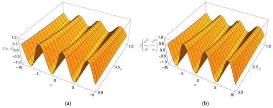
Figure 1.
Plots of the 3D solutions to Equation (42) obtained using the current methodology (a) and the exact solutions (b), which are shown at .
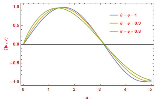
Figure 2.
The CDLSI method solution of for Equation (42) at .
Moreover, in Table 1 we present the absolute error of obtained by the CDLSI method at different values of .

Table 1.
The absolute error of obtained by the CDLSI method for Example 2 at different values of , , and .
Example 3.
Consider the KdV equation of the form
with the IC
and the BCs
This allows us to obtain the solution.
By applying the same steps in Example 2, one can obtain the following solution components:
As a result, we have the solution of Equation (44) as
We can see that if , then the exact solution is
The following figure (Figure 3) illustrates the 3D graph of the exact and approximate solutions of Example 3 at . In Figure 4, we sketch the solutions of for Equation (50) at
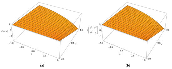
Figure 3.
Plots of the 3D solutions to Equation (50) obtained using the current methodology (a) and the exact solutions (b), which are shown at .
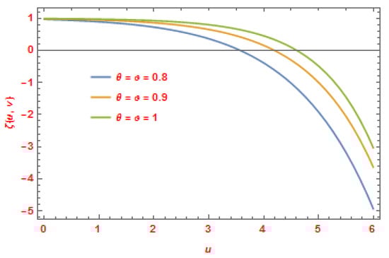
Figure 4.
The CDLSI solutions of for Equation (50) at .
Moreover, in Table 2 we present the absolute error of obtained by CDLSI at different values of , , and .
Table 2.
The absolute error of obtained by CDLSI for Example 3 at different values of , , and .
Example 4 .
Consider the Klein–Gordon equation of the form
with the ICs
and the BCs
This allows us to obtain the solution.
By applying the CDLST to Equation (52), the conformable Laplace transform to (53), and the conformable Sumudu transform to (54), we obtain
Taking the inverse transform of (55), we obtain
Now, by applying the iterative method, we substitute (26) in (56) and with the results in (30), (31), and (32) we obtain the following solution components:
As a result, we have the solution of Equation (52) as
We can see that if , then the exact solution is
The following figure (Figure 5) illustrates the 3D graph of the exact and approximate solutions of Example 4 at . In Figure 6, we sketch the solutions of
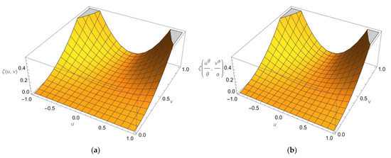
Figure 5.
Plots of the 3D solutions to Equation (60) obtained using the current methodology (a) and the exact solutions (b), which are shown at .
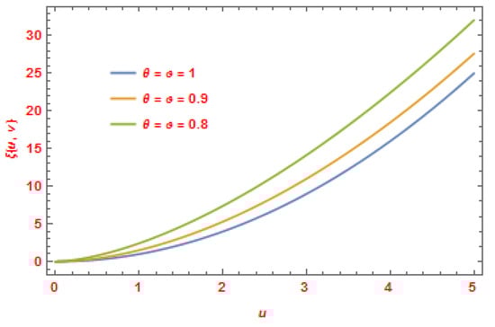
Figure 6.
The CDLSI solutions of for Equation (60) at .
Moreover, in Table 3 we present the absolute error of obtained by CDLSI for Example 4 at different values of , , and .
Table 3.
The absolute error of obtained by CDLSI for Example 4 at different values of , , and .
Example 5 .
Consider the telegraph equation of the form
with the Ics
and the BCs
Applying the same steps as in Example 5, we obtain the following solution components:
As a result, we have the solution of Equation (62) as
We can see that if, then the exact solution is
The following figure (Figure 7) illustrates the 3D graph of the exact and approximate solutions of Example 5 at . In Figure 8, we sketch the solutions of for Equation (68) at
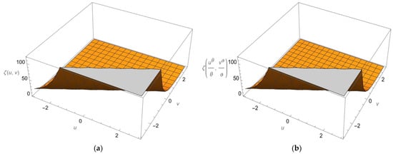
Figure 7.
Plots of the 3D solutions to Equation (68) obtained using the current methodology (a) and the exact solutions (b), which are shown at .
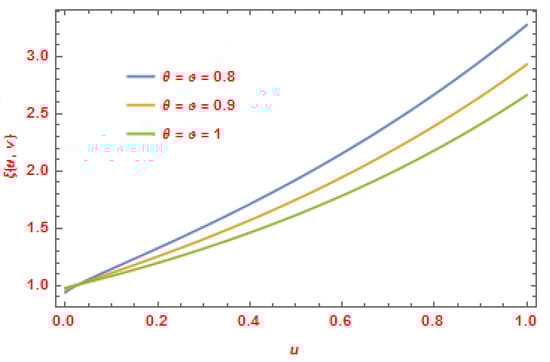
Figure 8.
The CDLSI solutions of for Equation (68) at .
Moreover, in Table 4 we present the absolute error of obtained by CDLSI at different values of , , and .
Table 4.
The absolute error of obtained by CDLSI for Example 5 at different values of , , and .
Example 6.
We consider the following nonlinear fractional equation in the sense of CFD:
with the Ics
and the BCs
This allows us to obtain the solution.
Operating the CDLST on (70) and the conformable Laplace transform on (71), we obtain
Taking the inverse transform of (73), we obtain
Now, applying the iterative method, we substitute (28) in (74) and with the results in (30), (31), and (32) we obtain the following solution components:
As a result, we have the solution of Equation (70) as:
The exact solution if is
The following figure (Figure 9) illustrates the 3D graph of the exact and approximate solutions of Example 6 at . In Figure 10, we sketch the solutions of for Equation (78) at
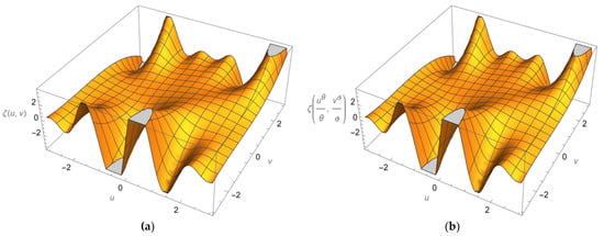
Figure 9.
Plots of the 3D solutions to Equation (78) obtained using the current methodology (a) and the exact solutions (b), which are shown at .
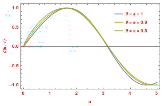
Figure 10.
The CDLSI solutions of for Equation (78) at .
Moreover, in Table 5 we present the absolute error of obtained by CDLSI at different values of , , and .
Table 5.
The absolute error of obtained by CDLSI for Example 6 at different values of , , and .
6. Results and Discussion
This part discusses the suggested method’s accuracy and applicability by comparing the approximate and exact solutions using graphs and tables. Figure 1, Figure 3, Figure 5, Figure 7 and Figure 9 depict the 3D plot solutions of Examples 2–6 obtained by the present method in comparison with the exact solutions at . These figures reveal that the approximate solutions obtained by the CDLSI method are almost identical to the exact solutions. Figure 2, Figure 4, Figure 6, Figure 8 and Figure 10 present comparisons of line plots of the approximate solutions from the proposed method and the exact solutions of Examples 2–6 for different values of and fractional-order values and . As we can see from the figures, the numerical solutions become close to the exact solutions when A comparative study between the exact and approximate solutions of each example in terms of absolute error at and at for different values of is provided in Table 1, Table 2, Table 3, Table 4 and Table 5. As observed from the figures and tables, it is confirmed that our method of solution converges quickly towards an exact solution.
7. Conclusions
The definition of the CDLST was introduced in this article. First, we applied the CDLST to a few particular functions. Following that, some theorems and properties connected to the CDLST were presented and proven. In order to gain precise solutions of a wide class of nonlinear conformable partial differential equations in the sense of conformable derivatives, we used the CDLST combined with the iterative approach to demonstrate the applicability and effectiveness of the suggested approach. For the strength of the outcomes, we sketched the solutions and compared them to the exact solutions in the integer case. We concluded that the suggested approach is effective, appropriate, trustworthy, and adequate to achieve the exact solutions of nonlinear conformable partial differential equations. In addition, the CDLSI method’s computations use less computing power than those of other similar techniques.
Author Contributions
Data curation, R.S., T.M.E., S.A.A. and A.Q.; formal analysis, S.A.A., R.S., T.M.E. and A.Q.; investigation, S.A.A., A.Q., R.S. and T.M.E.; methodology, S.A.A., R.S., T.M.E. and A.Q.; project administration, A.Q., T.M.E., R.S. and S.A.A.; resources, S.A.A., R.S., A.Q. and T.M.E.; writing—original draft, T.M.E., A.Q., R.S. and S.A.A.; writing—review and editing, S.A.A., R.S., T.M.E. and A.Q. All authors have read and agreed to the published version of the manuscript.
Funding
This research received no external funding.
Data Availability Statement
Not applicable.
Acknowledgments
The authors express their gratitude to the dear referees, who wish to remain anonymous, and the editor for their helpful suggestions, which improved the final version of this paper.
Conflicts of Interest
The authors declare no conflict of interest.
References
- Podlubny, I. Fractional Differential Equations; Academic Press: London, UK, 1999. [Google Scholar]
- Avci, D.; Iskender, E.; Ozdemir, N. Conformable heat equation on a radial symmetric plate. Therm. Sci. 2017, 21, 819–826. [Google Scholar] [CrossRef]
- Kilbas, A.A.; Srivastava, H.M.; Trujillo, J.J. Theory and Applications of Fractional Differential Equations; Elsevier: Amsterdam, The Netherlands, 2006. [Google Scholar]
- Khalil, R.; Al-Horani, M.; Yousef, A.; Sababheh, M. A new definition of fractional derivative. J. Comput. Appl. Math. 2014, 264, 65–70. [Google Scholar] [CrossRef]
- Hosseini, K.; Mayeli, P.; Ansari, R. Bright and singular soliton solutions of the conformable time-fractional Klein–Gordon equations with different nonlinearities. Waves Random Complex Media 2017, 26, 1–9. [Google Scholar] [CrossRef]
- Chen, C.; Jiang, Y.L. Simplest equation method for some time-fractional partial differential equations with conformable derivative. Comput. Math. Appl. 2018, 75, 2978–2988. [Google Scholar] [CrossRef]
- Hashemi, M.S. Invariant subspaces admitted by fractional differential equations with conformable derivatives. Chaos Solitons Fractals 2018, 107, 161–169. [Google Scholar] [CrossRef]
- Alfaqeih, S.; Mısırlı, E. Conformable double Laplace transform method for solving conformable fractional partial differential equations. Comput. Methods Differ. Equ. 2021, 9, 908–918. [Google Scholar]
- Osman, W.M.; Elzaki, T.M.; Siddig, N.A.A. Modified double conformable Laplace transform and singular fractional pseudo-hyperbolic and pseudo-parabolic equations. J. King Saud Univ.–Sci. 2021, 33, 101378. [Google Scholar] [CrossRef]
- Alfaqeih, S.; Misirli, E. On double Shehu transform and its properties with applications. Int. J. Anal. Appl. 2020, 18, 381–395. [Google Scholar]
- Deresse, A.T. Analytical solutions of one-dimensional nonlinear conformable fractional telegraph equation by reduced differential transform method. Adv. Math. Phys. 2022, 2022, 7192231. [Google Scholar] [CrossRef]
- Alfaqeih, S.; Kayijuka, I. Solving system of conformable fractional differential equations by conformable double Laplace decomposition method. J. Partial. Differ. Equ. 2020, 33, 275–290. [Google Scholar]
- Eltayeb, H.; Mesloub, S. Application of conformable Sumudu decomposition method for solving conformable fractional coupled burgers equation. J. Funct. Spaces 2021, 2021, 6613619. [Google Scholar]
- Bhanotar, S.A.; Kaabar, M.K.A. Analytical solutions for the nonlinear partial differential equations using the conformable triple Laplace transform decomposition method. Int. J. Differ. Equ. 2021, 2021, 9988160. [Google Scholar] [CrossRef]
- Bhanotar, S.A.; Belgacem, F.B.M. Theory and applications of distinctive conformable triple Laplace and Sumudu transforms decomposition methods. J. Partial. Differ. Equ. 2021, 35, 49–77. [Google Scholar]
- Deresse, A.T. Analytical solutions to two-dimensional nonlinear telegraph equations using the conformable triple Laplace transform iterative method. Adv. Math. Phys. 2022, 2022, 4552179. [Google Scholar] [CrossRef]
- Thabet, H.; Kendre, S. Analytical solutions for conformable space-time fractional partial differential equations via fractional differential transform. Chaos Solitons Fractals 2018, 109, 238–245. [Google Scholar] [CrossRef]
- Ahmed, S.A.; Elzaki, T.; Elbadri, M.; Mohamed, M.Z. Solution of partial differential equations by new double integral transform (Laplace—Sumudu transform). Ain Shams Eng. J. 2021, 12, 4045–4049. [Google Scholar] [CrossRef]
- Saadeh, R.; Qazza, A.; Burqan, A. On the double ARA-Sumudu transform and its applications. Mathematics 2022, 10, 2581. [Google Scholar] [CrossRef]
- Elzaki, T.; Ahmed, S.; Areshi, M.; Chamekh, M. Fractional partial differential equations and novel double integral transform. J. King Saud Univ.–Sci. 2022, 34, 101832. [Google Scholar] [CrossRef]
- Ahmed, S.A.; Qazza, A.; Saadeh, R. Exact solutions of nonlinear partial differential equations via the new double integral transform combined with iterative method. Axioms 2022, 11, 247. [Google Scholar] [CrossRef]
- Qazza, A.; Burqan, A.; Saadeh, R. Application of ARA-residual power series method in solving systems of fractional differential equations. Math. Prob. Eng. 2022, 2022, 47–62. [Google Scholar] [CrossRef]
- Saadeh, R.; Burqan, A.; El-Ajou, A. Reliable solutions to fractional Lane-Emden equations via Laplace transform and residual error function. Alex. Eng. J. 2022, 61, 10551–10562. [Google Scholar] [CrossRef]
- Qazza, A.; Burqan, A.; Saadeh, R.; Khalil, R. Applications on double ARA–Sumudu transform in solving fractional partial differential equations. Symmetry 2022, 14, 1817. [Google Scholar] [CrossRef]
- Mishra, H.K.; Nagar, A.K. He-Laplace method for linear and nonlinear partial differential equations. J. Appl. Math. 2012, 2012, 180315. [Google Scholar]
- Hamza, A.E.; Elzaki, T. Application of homotopy perturbation and Sumudu transform method for solving burgers equations. Am. J. Theor. Appl. Stat. 2015, 4, 480–483. [Google Scholar] [CrossRef]
- Hilal, E.; Elzaki, T. Solution of nonlinear partial differential equations by new Laplace variational iteration method. J. Funct. Spaces 2014, 2014, 790714. [Google Scholar] [CrossRef]
- Khan, Y.; Wu, Q. Homotopy perturbation transform method for nonlinear equations using He’s polynomials. Comput. Math. Appl. 2011, 61, 1963–1967. [Google Scholar] [CrossRef]
- Eltayeb, H.; Kilicman, A. A note on double Laplace transform and telegraphic equations. Abstr. Appl. Anal. 2013, 2013, 932578. [Google Scholar] [CrossRef]
- Huang, Y.Q.; Li, R.; Liu, W. Preconditioned descent algorithms for p-Laplacian. J. Sci. Comput. 2007, 32, 343–371. [Google Scholar] [CrossRef]
- Al-Luhaibi, M.S. New iterative method for fractional gas dynamics and coupled burger’s equations. Sci. World J. 2015, 2015, 153124. [Google Scholar] [CrossRef]
- Chen, X.; Wang, C.; Wise, S.M. A preconditioned steepest descent solver for the Cahn-Hilliard equation with variable mobility. Int. J. Numer. Anal. Model. 2022, 19, 839–863. [Google Scholar]
- Feng, W.; Salgado, A.J.; Wang, C.; Wise, S.M. Preconditioned steepest descent methods for some nonlinear elliptic equations involving p-Laplacian terms. J. Comput. Phys. 2017, 334, 45–67. [Google Scholar] [CrossRef]
- Zhang, J.; Wang, C.; Wise, S.M.; Zhang, Z. Structure-preserving, energy stable numerical schemes for a liquid thin film coarsening model. SIAM J. Sci. Comput. 2021, 43, 1248–1272. [Google Scholar] [CrossRef]
- Feng, W.; Wang, C.; Wise, S.M.; Zhang, Z. A second-order energy stable backward differentiation formula method for the epitaxial thin film equation with slope selection. Numer. Methods Partial. Differ. Equ. 2018, 34, 1975–2007. [Google Scholar] [CrossRef]
- Daftardar-Gejji, V.; Jafari, H. An iterative method for solving nonlinear functional equations. J. Math. Anal. Appl. 2006, 316, 753–763. [Google Scholar] [CrossRef]
- Ali, L.; Islam, S.; Gul, T.; Amiri, I.S. Solution of nonlinear problems by a new analytical technique using Daftardar-Gejji and Jafari polynomials. Adv. Mech. Eng. 2019, 11, 10. [Google Scholar] [CrossRef]
- Dhunde, R.R.; Waghamare, G.L. Double Laplace iterative method for solving nonlinear partial differential equations. New Trends Math. Sci. 2019, 7, 138–149. [Google Scholar] [CrossRef]
- Dhunde, R.R.; Waghamare, G.L. Analytical solution of the nonlinear Klein-Gordon equation using double Laplace transform and iterative method. Am. J. Comput. Appl. Math. 2016, 6, 195–201. [Google Scholar]
- Wazwaz, A.M. Partial Differential Equations and Solitary Wave’s Theory; Higher Education Press: Beijing, China; Springer: Berlin/Heidelberg, Germany, 2009. [Google Scholar]
Disclaimer/Publisher’s Note: The statements, opinions and data contained in all publications are solely those of the individual author(s) and contributor(s) and not of MDPI and/or the editor(s). MDPI and/or the editor(s) disclaim responsibility for any injury to people or property resulting from any ideas, methods, instructions or products referred to in the content. |
© 2022 by the authors. Licensee MDPI, Basel, Switzerland. This article is an open access article distributed under the terms and conditions of the Creative Commons Attribution (CC BY) license (https://creativecommons.org/licenses/by/4.0/).