Ab Initio Calculations of Transport and Optical Properties of Dense Zr Plasma Near Melting

Abstract

The dynamic electrical conductivity of dense Zr plasma near melting is calculated using ab initio molecular dynamics and the Kubo–Greenwood formula. The antisymmetrization of the electronic wave function is considered with the determinant of one-electron wave functions; exchange and correlation effects are treated via an exchange–correlation functional. Optical properties are restored using the Kramers–Kronig transformation. The influence of computational parameters and inner shell electrons on the results is thoroughly investigated. We demonstrate the convergence of our computations and analyze comparison with experimental data.

1. Introduction

Zirconium finds many applications because this metal is refractory (the melting temperature $T_{\mathrm{m}}=2127$ K [1]), hard, and resistant to chemically aggressive environments. It applies in metallurgy as a composite component of steels, and as molds for molten metals. Zirconium alloys are applied in the nuclear industry for nuclear reactor fuel cladding because of their low neutron-capture cross-section and resistance to corrosion under service conditions. Zirconium also has a lot of applications in space and aeronautic industries (ZrO is one of the perspective materials for some details of jet engines), and medicine (dental and bone prostheses). These are the reasons why the study of zirconium properties is the subject of great interest in science and technology.

The properties of Zr near melting were studied experimentally and theoretically. The work [2] provides the first experimental measurements of the melting curve of zirconium at pressures up to 29 GPa. Though significant progress has been achieved in the measurements of melting during the last two decades there are still essential experimental difficulties for refractory metals even at low pressures [3]. The lattice structure and thermodynamic properties of $\beta$-phase Zr were studied by classical molecular dynamics simulations [4]. The properties of Zr in the vicinity of the binodal curve were studied in [5,6] using the similarity laws. Ab initio molecular dynamics simulations were used to explore the local structure of dense Zr plasma melting and its evolution upon undercooling to describe neutron scattering experiments [7,8].

Nevertheless, experimental data on the transport and optical properties of liquid zirconium are almost lacking. The resistivity of solid zirconium was measured in many works in the range of temperature 1–2127 K; these data were collected by Desai [9]. In dynamical experiments by Korobenko et al. [10,11,12] the electrical explosion of Zr foils and wires were applied to widen the range of resistivity measurements in liquid zirconium up to 4100 K. The optical properties of liquid Zr are poorly known and the data are available only near the melting temperature [13,14,15,16,17] while in the solid phase a lot of experiments can be found [18,19,20,21,22]. Meanwhile, transport and optical properties of dense metallic plasma are crucial for magnetohydrodynamic and radiative magnetoplasmadynamic codes [23].

On the other hand, ab initio calculations, which are based on quantum molecular dynamics (QMD), finite-temperature density functional theory (DFT), and the Kubo–Greenwood formula, allow us to obtain transport and optical properties from first principles in the wide range of temperatures [24,25,26,27,28,29,30,31,32,33,34,35]. In such calculations, liquid metal is treated as a strongly coupled degenerate plasma. This means that the electronic subsystem should be described by a wave function that is antisymmetric in the permutation of any two electrons [36]. In DFT this is usually achieved by using a determinant composed of one-electron wave functions. For the exchange interaction energy and correlation effects, however, approximations of complicated quantum many-particle calculations exist which are traditionally called exchange-correlation functionals [37]. This simplification speeds up computations dramatically while providing good accuracy.

In this paper, we present the first ab initio calculation of the dynamic electrical conductivity of liquid zirconium. We also investigate the influence of simulation parameters on the obtained results and restoration of optical properties.

2. Computational Methods

2.1. Problem Formulation

In this work, calculations consist of three subsequent stages.

At the first stage, a QMD simulation is performed. In QMD the initial parameters are temperature ($T_{\mathrm{e}}=T_{\mathrm{i}}$, where $T_{\mathrm{e}}$ and $T_{\mathrm{i}}$ are the temperatures of electrons and ions, accordingly) and density $\rho$. The atoms of the substance are placed in a supercell with the lattice parameter corresponding to a given density. Other parameters of the simulation (k-points grid size, number of bands, cutoff energy for plane waves, etc.) are chosen to provide the convergence of thermodynamic properties. Then the QMD simulation is carried out at a given temperature (the temperature is maintained by a thermostat) and the ionic trajectories are calculated. At each ionic step, the electronic structure is calculated in the framework of finite-temperature DFT. The ionic positions are determined using the Hellman–Feynman forces obtained from the electronic structure calculation in which the Born–Oppenheimer approximation is applied. After reaching equilibrium, a set of ionic configurations is selected for the next stages of the study. The number of configurations is chosen to ensure the convergence of the calculated properties, while the distance between neighboring configurations should be large enough to ensure the absence of correlations. In this work, 9 configurations were chosen for averaging after the system had reached the equilibrium state, and every 300th QMD step was chosen.

At the second stage, more precise additional DFT calculations of electronic structure for the selected configurations are performed. At this stage, we use other values of some parameters of simulation (finer k-points grid, more number of bands) which can provide better accuracy compared with the calculations at the first stage. As a result of the second stage, we have the eigenstates and eigenvalues for electronic bands and corresponding Fermi-weights.

The first and second stages are made using the VASP package [38,39].

At the third stage, transport and optical properties are calculated. The real part of the dynamic complex electrical conductivity $\sigma \left(\omega \right)$ is reconstructed using the Kubo–Greenwood formula implemented in the GreeKuP code [30], while the imaginary part can be restored using the Kramers–Kronig transform (both methods are described in detail below in this section). At known $\sigma \left(\omega \right)={\sigma }_1\left(\omega \right)+i{\sigma }_2\left(\omega \right)$ we can obtain optical properties depending on the radiation frequency $\omega$:

• the complex dielectric constant $\epsilon \left(\omega \right)={\epsilon }_1\left(\omega \right)+i{\epsilon }_2\left(\omega \right)$ as

  $${\epsilon }_1\left(\omega \right)=1-\frac{{\sigma }_2\left(\omega \right)}{\omega {\epsilon }_0},{\epsilon }_2\left(\omega \right)=\frac{{\sigma }_1\left(\omega \right)}{\omega {\epsilon }_0},$$

  where ${\epsilon }_0$ is the vacuum permittivity;
• the complex refractive index $n\left(\omega \right)+ik\left(\omega \right)$ as

  $$n\left(\omega \right)=\sqrt{\frac{\left|\epsilon \left(\omega \right)\right|+{\epsilon }_1\left(\omega \right)}{2}},k\left(\omega \right)=\sqrt{\frac{\left|\epsilon \left(\omega \right)\right|-{\epsilon }_1\left(\omega \right)}{2}};$$
• the normal spectral reflectivity as

  $$R\left(\omega \right)=\frac{{\left(1-n\left(\omega \right)\right)}^2+k{\left(\omega \right)}^2}{{\left(1+n\left(\omega \right)\right)}^2+k{\left(\omega \right)}^2};$$
• the absorption coefficient as

  $$\alpha \left(\omega \right)=2k\left(\omega \right)\frac{\omega }{c},$$

  where c is the speed of light in a vacuum;
• the normal spectral emissivity as

  $$\mathcal{E}\left(\omega \right)=1-R\left(\omega \right).$$

2.2. Kubo–Greenwood Formula

The dynamic complex electrical conductivity $\sigma \left(\omega \right)={\sigma }_1\left(\omega \right)+i{\sigma }_2\left(\omega \right)$ is the coefficient between the current density ${\mathbf{j}}_{\omega }$ and the applied electric field ${\mathbf{E}}_{\omega }$ of the frequency $\omega$: ${\mathbf{j}}_{\omega }=\sigma \left(\omega \right){\mathbf{E}}_{\omega }$.

The Kubo–Greenwood formula [24,26,30,40]

$${\sigma }_1\left(\omega \right)=\frac{2\pi e^2{\hslash }^2}{3m_{\mathrm{e}}^2\omega \mathsf{\Omega }}\sum _{i,j,\alpha ,\mathbf{k}}\left(W\left(\mathbf{k}\right)|\langle {\mathsf{\Psi }}_{i,\mathbf{k}}|{\nabla }_{\alpha }|{\mathsf{\Psi }}_{j,\mathbf{k}}\rangle {|}^2\left(f\left({ϵ}_{i,\mathbf{k}}\right)-f\left({ϵ}_{j,\mathbf{k}}\right)\right)\delta ({ϵ}_{j,\mathbf{k}}-{ϵ}_{i,\mathbf{k}}-\hslash \omega )\right)$$

(1)

is used for calculating the real part of the dynamic electrical conductivity ${\sigma }_1\left(\omega \right)$ when $\omega \ne 0$. In this formula ${\sigma }_1\left(\omega \right)$ can be treated as the energy absorption at the frequency $\omega$. Here ${\mathsf{\Psi }}_{i,\mathbf{k}}$ are the electronic eigenfunctions and ${ϵ}_{i,\mathbf{k}}$ are the electronic eigenvalues for the electronic band at a given $\mathbf{k}$-point in the Brillouin zone; $W\left(\mathbf{k}\right)$ is the $\mathbf{k}$-point weight in the Brillouin zone, $f\left({ϵ}_{i,\mathbf{k}}\right)$ is the Fermi distribution function; $\mathsf{\Omega }$ is the supercell volume, e and $m_{\mathrm{e}}$ are the electronic charge and mass, accordingly. To find the absorption ${\sigma }_1\left(\omega \right)$ we should take into account all transitions between all possible states i and j. Only levels with energy difference $\hslash \omega$ make a contribution to energy absorption at the frequency $\omega$; so, a $\delta$ function is included in the Kubo–Greenwood formula. The $\delta$ function is replaced by a Gaussian with a broadening of $\mathsf{\Delta }E$ = 0.05 eV. The squared matrix elements $|\langle {\mathsf{\Psi }}_i|{\nabla }_{\alpha }|{\mathsf{\Psi }}_j{\rangle |}^2$ represent the intensity of every transition between electronic energy levels (${\nabla }_{\alpha }$ is the velocity operator along each spatial direction $\alpha$).

2.3. Kramers–Kronig Transform

The real and imaginary part of an analytic in the upper half-plane function $\sigma \left(\omega \right)={\sigma }_1\left(\omega \right)+i{\sigma }_2\left(\omega \right)$ are connected via the Kramers–Kronig transform (KKT): at a known real part ${\sigma }_1\left(\omega \right)$ the relation

$${\sigma }_2\left(\omega \right)=-\frac{2\omega }{\pi }\mathcal{P}{\int }_0^{\infty }\frac{{\sigma }_1\left({\omega }^{\prime }\right)}{{\omega }^{\prime 2}-{\omega }^2}d{\omega }^{\prime }$$

(2)

can be used to find the imaginary part ${\sigma }_2\left(\omega \right)$ of this function. Here $\mathcal{P}$ denotes the Cauchy principal value. For any stable physical systems, causality implies the condition of analyticity, and conversely, analyticity implies causality of the corresponding stable physical system [41].

In a practical calculation, the upper limit of integration in Formula (2) is some large finite value ${\omega }_{\max }$, and to avoid the divergence in the integrand a small parameter $\eta$ is introduced in the denominator of the integrand

$${\sigma }_2\left(\omega \right)\approx -\frac{2\omega }{\pi }{\int }_0^{{\omega }_{\max }}\frac{{\sigma }_1\left({\omega }^{\prime }\right)}{{\omega }^{\prime 2}-{\omega }^2+i\eta }d{\omega }^{\prime }.$$

(3)

For performing the KKT (numerical calculation of the Cauchy principal value of the integral) a parallel C++ program was developed by the authors [42]. The function ${\sigma }_1\left(\omega \right)$ is given as a one-dimension array with different values ${\sigma }_i$ for different values ${\omega }_i$ with a step $\mathsf{\Delta }\omega$. As ${\sigma }_1\left(\omega \right)$ may have sawtooth-like behavior at low temperatures due to the small size of the system we use the trapezoidal rule for integration to avoid additional interpolation errors. In this program, we can set a different upper integration limit ${\omega }_{\max }$ and change the integration step $\mathsf{\Delta }\omega$. The cubic spline of the original function ${\sigma }_1\left(\omega \right)$ is used in the case of a small integration step $\mathsf{\Delta }\omega$ (implemented using GSL library). A user can also increase the upper integration limit ${\omega }_{\max }$ beyond the maximum frequency value of the array. In this case, additional elements of the ${\sigma }_1\left(\omega \right)$ array are populated with the last value of the original array. Convergence according to the parameter $\eta$ was tested and achieved at $\eta \le {10}^{-6}$.

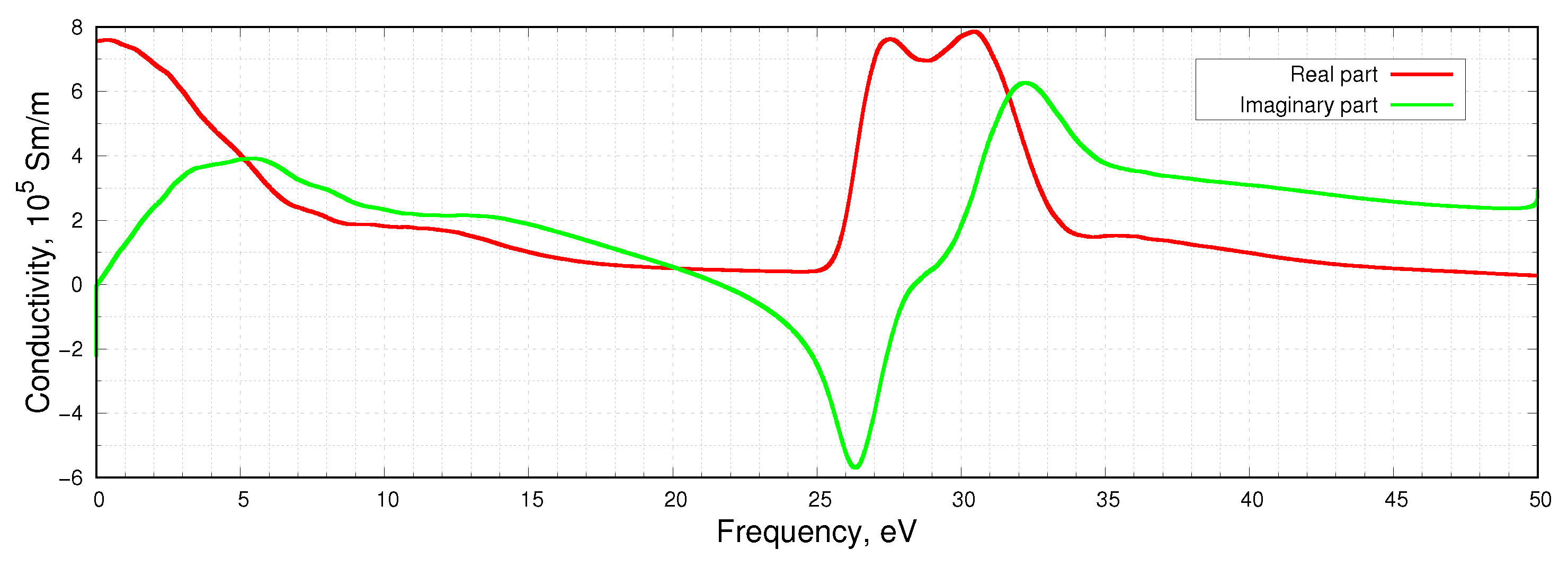
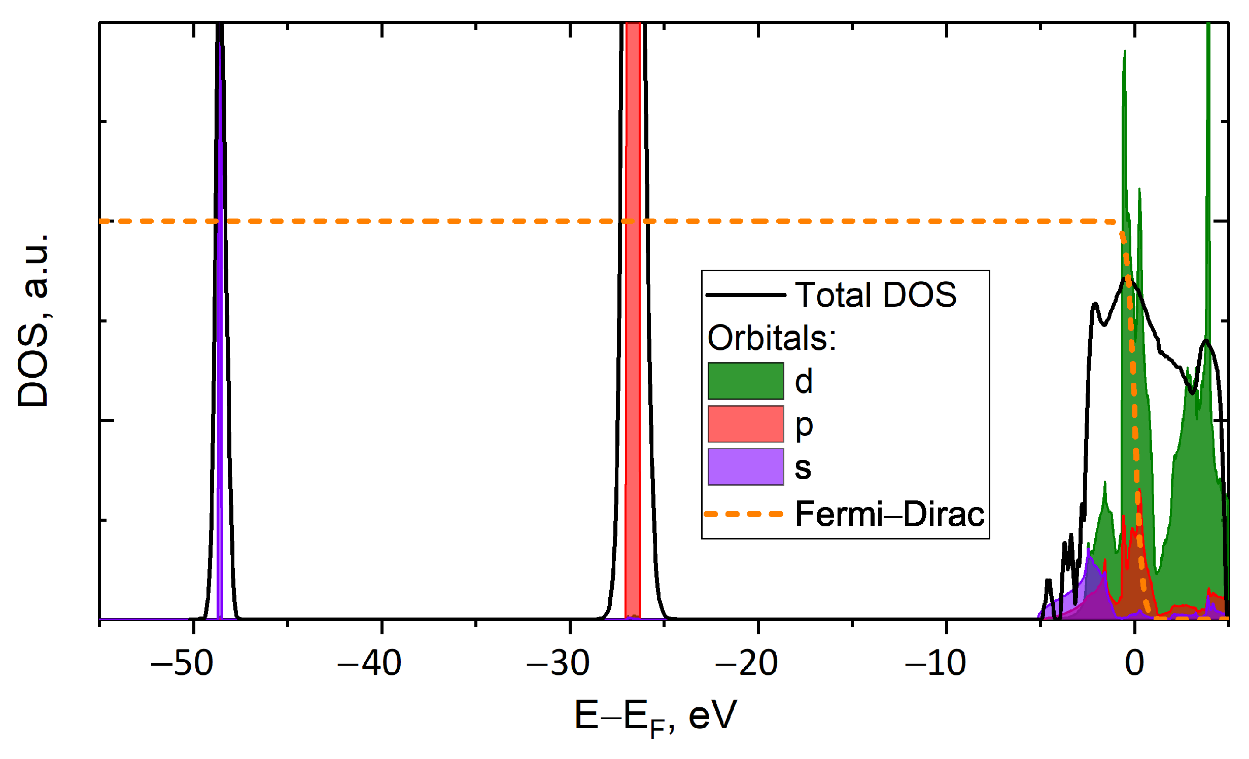
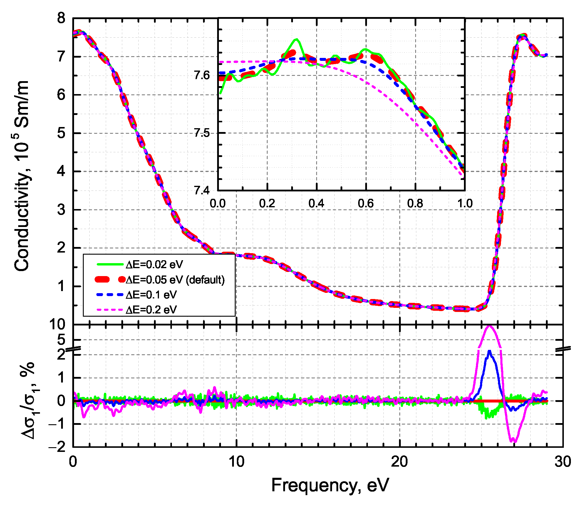
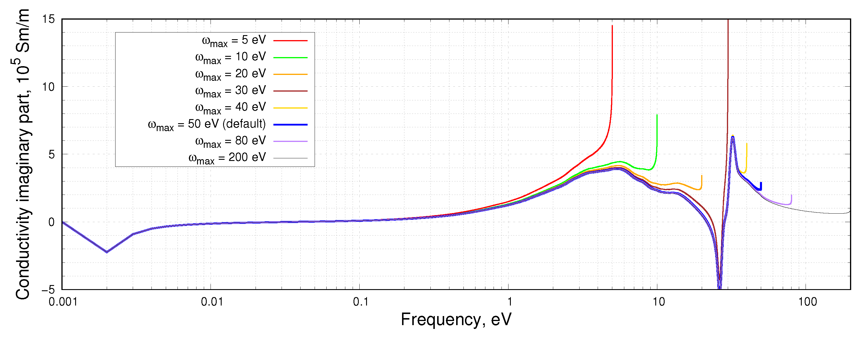
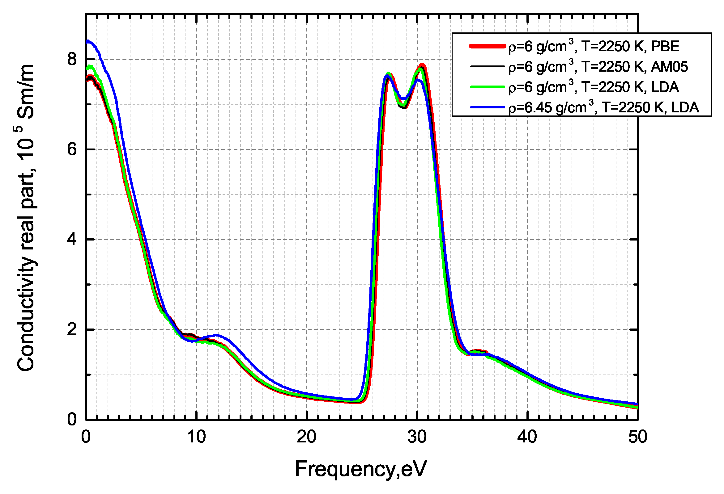
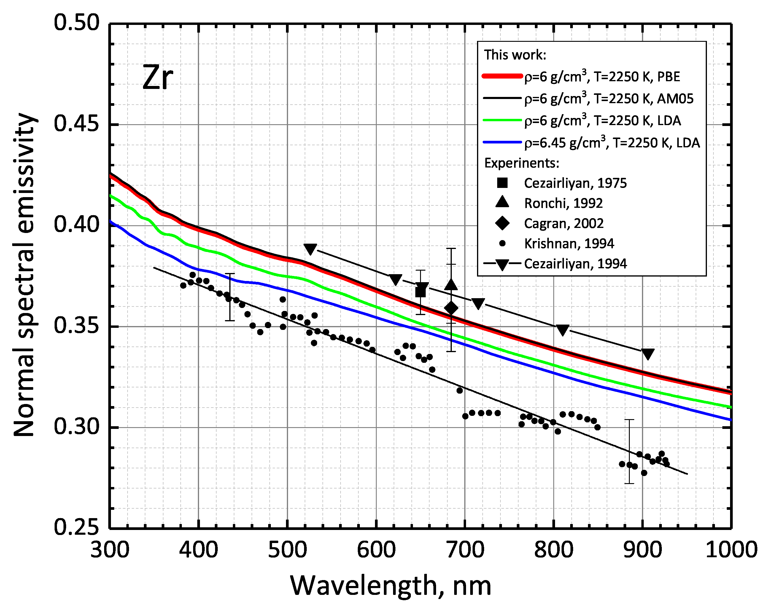
3. Results and Discussion

In this work 250 atoms of Zr in the supercell with periodical boundary conditions are simulated, the density is 6 g/cm${}^3$, and the temperature is 2250 K. Convergence of thermodynamic and transport properties on the number of atoms was achieved. QMD simulation was performed using the Baldereschi mean value point for the Brillouin zone evaluation. The average pressure obtained in the QMD calculation is about zero. At the second stage of calculation (see Section 2.1) 2 × 2 × 2 $\mathbf{k}$-points grid in the Brillouin zone was used. The cutoff energy was set to 400 eV. The convergence of transport properties on the number of $\mathbf{k}$-points was also checked. The number of bands at this stage was chosen to provide the range of frequencies for ${\sigma }_1$ from 0 up to ${\omega }_{\max }=50$ eV. So, in our case, 8000 orbitals were taken in the DFT calculation with about 6000 unoccupied ones to account for high-energy transitions in the Kubo–Greenwood Formula (1).

The behavior of the real and imaginary parts of the dynamic electrical conductivity in the range of frequencies 0–50 eV is shown in Figure 1. The PAW potential for Zr with 12 valence electrons was used in our calculation, so the impact of the inner shell electrons (4s4p) on electrical conductivity may be observed. Indeed, ${\sigma }_1\left(\omega \right)$ demonstrates a pronounced hump in the region of 25–33 eV. To analyze the cause, we derive the electronic density of states (DOS) from the QMD eigenenergies. The projected DOS, obtained from the decomposition of the wavefunctions by spherical harmonics, for the bcc lattice with the same density is also shown in Figure 2 to help assess the contribution of individual orbitals. We can conclude that the 4p-electrons are the reason for the hump in the real part of electrical conductivity in Figure 1.

The generalized gradient approximation of Perdew, Burke, and Ernzerhof [43] is used as the main exchange-correlation (XC) functional in our calculations, since it provides the best agreement with the experimental normal density of Zr [44]. Nevertheless, below we will present a comparison of the calculation results with other XC-functionals as well.

The Gaussian broadening $\mathsf{\Delta }E$ was chosen to provide a smooth ${\sigma }_1$ profile and convergence of calculated ${\sigma }_1(\omega =0)\equiv {\sigma }_{DC}$. If we decrease the Gaussian broadening $\mathsf{\Delta }E$, then the dependence ${\sigma }_1\left(\omega \right)$ becomes fluctuating, see Figure 3. The ${\sigma }_1(\omega =0)$ values obtained by extrapolating the ${\sigma }_1\left(\omega \right)$-curve to zero frequency, differ less than 0.5% at different $\mathsf{\Delta }E$. Meanwhile, our calculation shows that QMD with the Kubo–Greenwood formula underestimates the electrical resistivity $\rho =1/{\sigma }_{DC}$ of liquid Zr at 2250 K by more than 6% in comparison with the available experiments, specifically 132 $\mathsf{\mu }\mathsf{\Omega }·$cm in our calculation compared to measured 141.7 [9] at 2127 K, 139.7 [11] and 148.3 $\mathsf{\mu }\mathsf{\Omega }·$cm [10] at 2250 K, correspondingly.

Further study was devoted to the investigation of the dependence of optical properties (mainly, normal spectral emissivity) on the integration range $[0;{\omega }_{\max }]$ (see Formula (3)) and on the integration step $\mathsf{\Delta }\omega$.

The behavior of ${\sigma }_2\left(\omega \right)$ corresponding to different integration ranges is shown in Figure 4, while Figure 5 represents the behavior of ${\sigma }_2\left(\omega \right)$ calculated with different integration steps.

Through the analysis of these figures, we can conclude that the integration range influences the imaginary part of dynamic conductivity in the range of high frequencies, whereas the integration step affects the imaginary part of dynamic conductivity in the range of low frequencies.

The dependence of the calculated normal spectral emissivity on the upper integration limit ${\omega }_{\max }$ is shown in Figure 6. The calculation of normal spectral emissivity $\mathcal{E}$ at a wavelength of 900 nm (corresponds to 1.3776 eV) for liquid Zr was analyzed. We vary the upper integration limit from 5 to 50 eV using the original calculated ${\sigma }_1\left(\omega \right)$ (see Figure 1) and beyond that up to 10${}^4$ eV using different assumptions. The real part of the dynamic conductivity ${\sigma }_1\left(\omega \right)$ is also shown (the red dashed line corresponds to the original calculated ${\sigma }_1\left(\omega \right)$). We can see a double peak on the ${\sigma }_1\left(\omega \right)$-curve in the vicinity of $\omega =30$ eV, so, varying the integration range, we can take this peak into account (if we set ${\omega }_{\max }\ge 40$ eV) or not (${\omega }_{\max }\le 20$ eV). We found that the inclusion of the peak insignificantly (less than 0.5%) changes the calculated emissivity value (red line with open dots).

In this figure, three different options of integration range continuation up to 10${}^4$ eV are also considered. As the first option (blue dashed line), we cut the ${\sigma }_1\left(\omega \right)$-curve at $\omega =24$ eV, then we extend the ${\sigma }_1\left(\omega \right)$-curve using the value ${\sigma }_1\left(24\mathrm{eV}\right)=$ 40,537 Sm/m. The corresponding calculated $\mathcal{E}$ is shown as the open blue dots. As the second option (green dashed line), we extend the ${\sigma }_1\left(\omega \right)$-curve after $\omega =50$ eV using the last value ${\sigma }_1\left(50\mathrm{eV}\right)=$ 27,748 Sm/m. The corresponding calculated $\mathcal{E}$ is shown as the open green dots. Finally, as the third option (olive dashed line), we extend the ${\sigma }_1\left(\omega \right)$-curve after $\omega =50$ eV using the maximum value of the ${\sigma }_1\left(\omega \right)$-curve peak: ${\sigma }_1\left(30.451\mathrm{eV}\right)=$ 785,802 Sm/m. The corresponding calculated $\mathcal{E}$ is shown as the open olive dots.

In the first and second cases, we can see that the continuation of the ${\sigma }_1\left(\omega \right)$ with a constant value practically does not change (<0.1%) the calculated emissivity (insignificant rising of the blue and green line with open dots). The third option can be considered as an attempt to analyze the influence of deep-lying inner-shell electrons on the calculation of optical properties and to obtain an upper estimate for the 900 nm normal spectral emissivity for liquid Zr at 2250 K. We can see that the emissivity increases no more than 1.1% compared to the emissivity value calculated using the original ${\sigma }_1$ (olive line with open dots).

The influence of the integration step on the accuracy of the normal spectral emissivity calculation is shown in Figure 7. The yellow point shows the emissivity calculated using the default integration step ($\mathsf{\Delta }{\omega }_0=0.001$ eV), the green line shows similar calculations with bigger $\mathsf{\Delta }\omega$, the magenta line represents the cases when we reduce $\mathsf{\Delta }\omega$ in comparison with $\mathsf{\Delta }{\omega }_0$, find the corresponding ${\sigma }_1$ values by the cubic spline interpolation and then calculate the emissivity using this reduced $\mathsf{\Delta }\omega$. The blue line shows the error (which is the difference between the value of emissivity at $\mathsf{\Delta }\omega$ and $\mathsf{\Delta }{\omega }_{\min }=5\times {10}^{-6}$ eV). We can see that the $\mathsf{\Delta }\omega$ influence becomes unimportant when $\mathsf{\Delta }\omega \le 0.01$ eV (in this case the error $\lesssim 0.1\%$).

Returning to the influence of the Gaussian broadening $\mathsf{\Delta }E$ on the recovery of optical properties, Figure 8 illustrates the deviation from the emissivity default value (when $\mathsf{\Delta }E=0.05$ eV). As can be seen, $\mathsf{\Delta }E$ has a very negligible effect on the calculated $\mathcal{E}$.

Finally, we analyze the effect of an XC-functional on the calculated properties using well-known non-empirical functionals: PBE, LDA [45], and AM05 [46]. We provide a comparison for the same ions configurations obtained with PBE to show a direct impact of an XC-functional on the optical properties restoration. However, since the choice of an XC-functional has a significant influence on pressure, we have added the calculation for 6.45 g/cm${}^3$ and 2250 K, which provides near-zero pressure for liquid Zr with LDA.

We found negligible differences between PBE and AM05, while LDA gives a noticeable difference in ${\sigma }_1$ calculations, see Figure 9. However, this difference has a limited effect on the calculated optical properties. The comparison of the calculated normal spectral emissivity of liquid Zr with experimental data in the vicinity of $T_{\mathrm{m}}$ is shown in Figure 10. We can see that the slopes of $\mathcal{E}\left(\lambda \right)$ obtained in this work using different XC-functionals are consistent with the linear fit of the experimental data by Krishnan et al. [16] and Cezarliyan et al. [47]. The values of normal spectral emissivity from first-principle calculations with PBE and AM05 functionals agree better with other experiments for $\lambda =650$ [13] and 684.5 nm [14,17] than the results obtained using LDA.

4. Conclusions

Our conclusions are as follows:

• We have presented the dynamic electrical conductivity of dense Zr plasma at $T=2250$ K and $\rho =6$ g/cm${}^3$ using the QMD approach and Kubo–Greenwood formula for the first time.
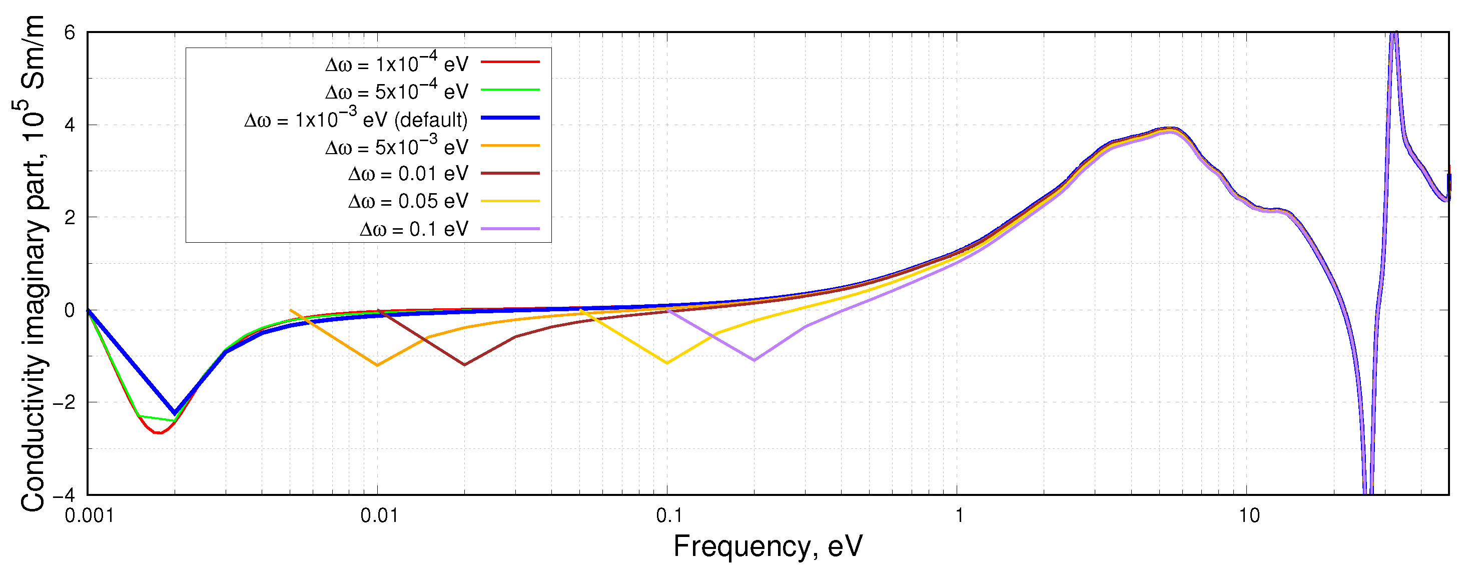
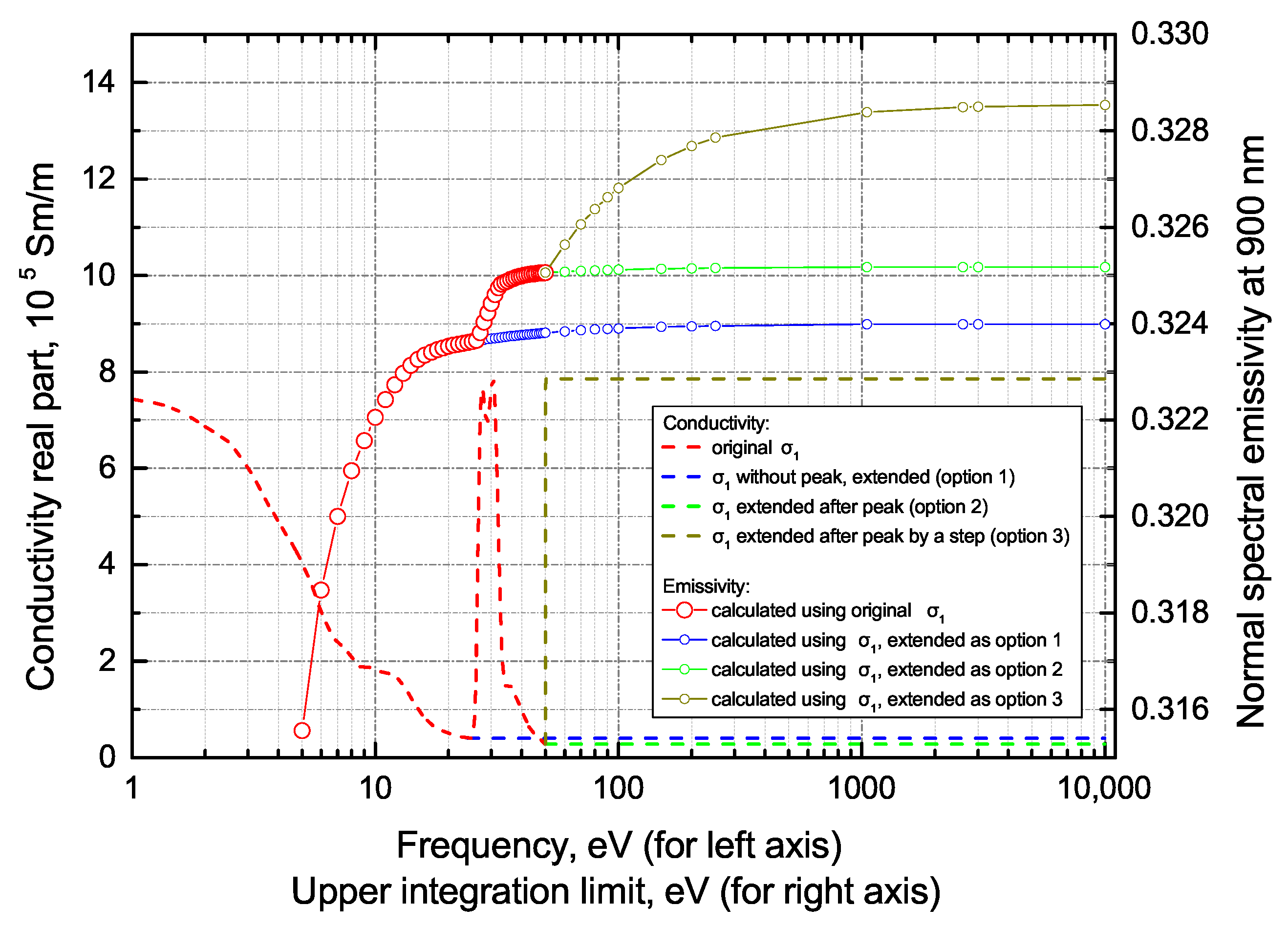
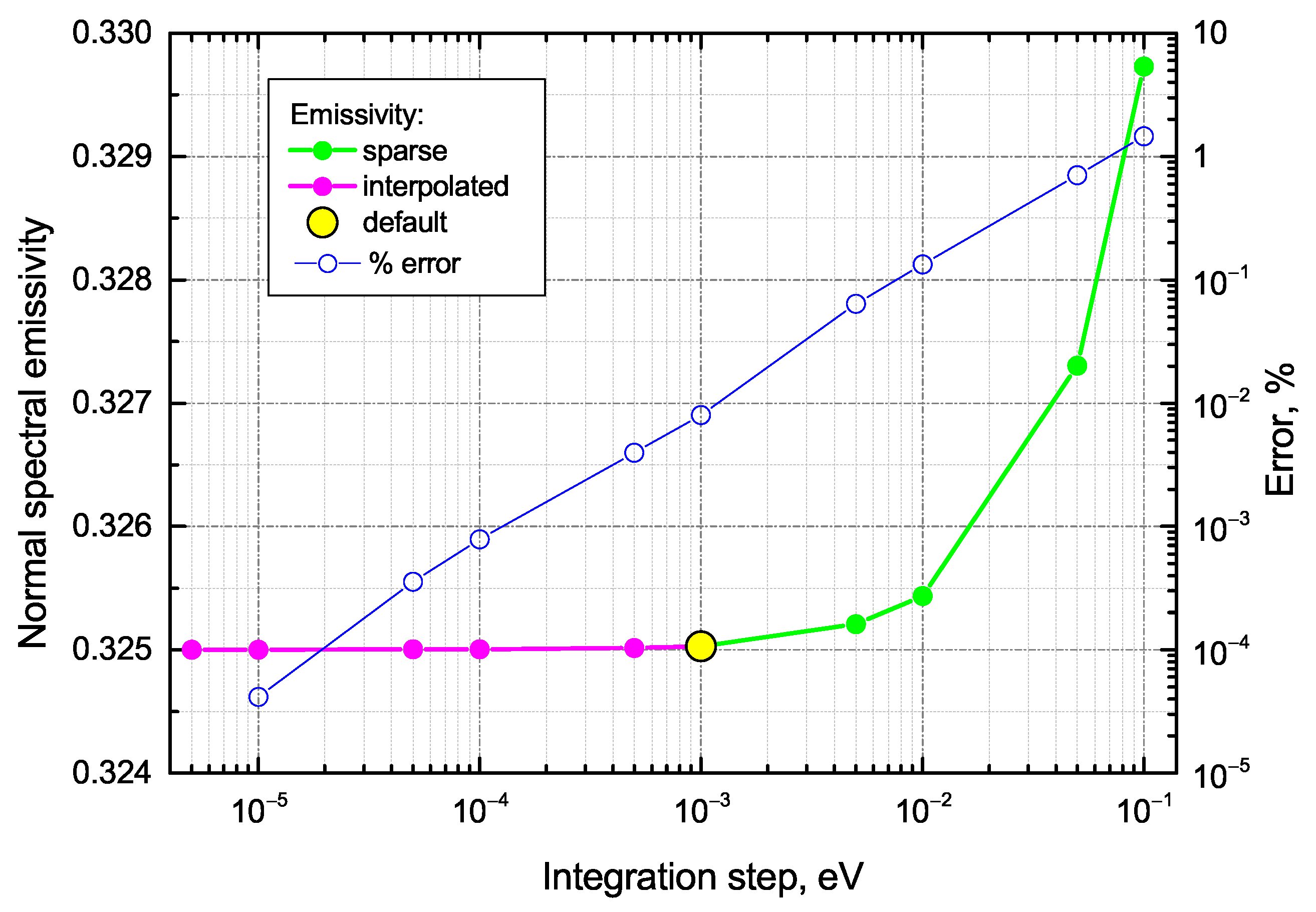
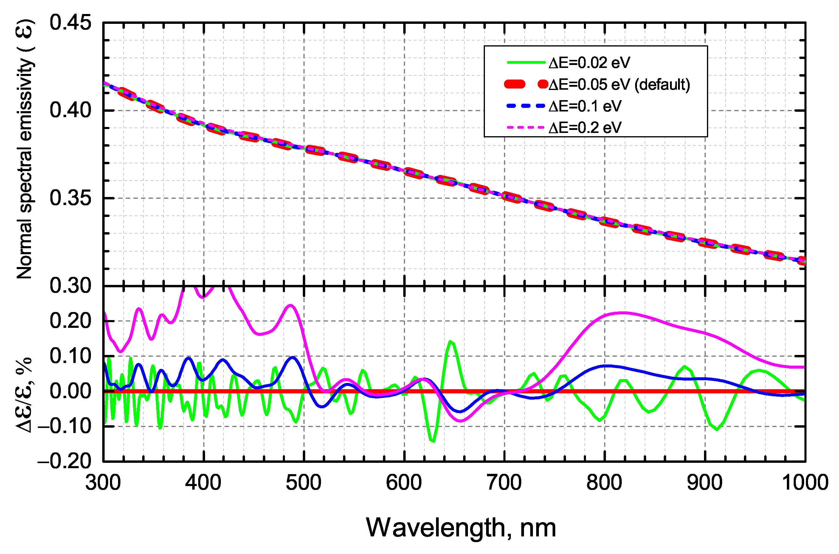
• We have analyzed the influence of simulation parameters of the numerical integration (integration range, integration step) in KKT and the choice of an exchange-correlation functional on the obtained results using normal spectral emissivity as an example.
• We have shown that the inner shell electrons give a limited contribution to the optical properties, so taking into account only the valence electrons provides a good estimate for transport and optical properties.
• We have demonstrated good agreement with the results of our calculations with experiments.

References

1. Arblaster, J.W. Thermodynamic properties of zirconium. CALPHAD Comput. Coupling Phase Diagrams Thermochem. 2013, 43, 32–39. [Google Scholar] [CrossRef]
2. Pigott, J.S.; Velisavljevic, N.; Moss, E.K.; Draganic, N.; Jacobsen, M.K.; Meng, Y.; Hrubiak, R.; Sturtevant, B.T. Experimental melting curve of zirconium metal to 37 GPa. J. Phys. Condens. Matter 2020, 32, 355402. [Google Scholar] [CrossRef] [PubMed]
3. Boikov, A.; Payor, V. The Present Issues of Control Automation for Levitation Metal Melting. Symmetry 2022, 14, 1968. [Google Scholar] [CrossRef]
4. Smirnova, D.E.; Starikov, S.V.; Gordeev, I.S. Evaluation of the structure and properties for the high-temperature phase of zirconium from the atomistic simulations. Comput. Mater. Sci. 2018, 152, 51–59. [Google Scholar] [CrossRef]
5. Apfelbaum, E.M.; Vorob’ev, V.S. Correspondence between the Critical and the Zeno-Line Parameters for Classical and Quantum Liquids. J. Phys. Chem. B 2009, 113, 3521–3526. [Google Scholar] [CrossRef]
6. Apfelbaum, E.M.; Vorob’ev, V.S. The Wide-Range Method to Construct the Entire Coexistence Liquid–Gas Curve and to Determine the Critical Parameters of Metals. J. Phys. Chem. B 2015, 119, 11825–11832. [Google Scholar] [CrossRef]
7. Jakse, N.; Pasturel, A. Local Order of Liquid and Supercooled Zirconium by Ab Initio Molecular Dynamics. Phys. Rev. Lett. 2003, 91, 195501. [Google Scholar] [CrossRef]
8. Jakse, N.; Bacq, O.L.; Pasturel, A. Short-range order of liquid and undercooled metals: Ab initio molecular dynamics study. J. Non-Cryst. Solids 2007, 353, 3684–3688. [Google Scholar] [CrossRef]
9. Desai, P.D.; James, H.M.; Ho, C.Y. Electrical Resistivity of Vanadium and Zirconium. J. Phys. Chem. Ref. Data 1984, 13, 1097–1130. [Google Scholar] [CrossRef]
10. Korobenko, V.N.; Savvatimskii, A.I. Temperature Dependence of the Density and Electrical Resistivity of Liquid Zirconium up to 4100 K. High Temp. 2001, 39, 525–531. [Google Scholar] [CrossRef]
11. Korobenko, V.; Savvatimski, A.; Sevostyanov, K. Experimental investigation of solid and liquid zirconium. High Temp. High Press. 2001, 33, 647–658. [Google Scholar] [CrossRef]
12. Korobenko, V.N.; Agranat, M.B.; Ashitkov, S.I.; Savvatimskiy, A.I. Zirconium and iron densities in a wide range of liquid states. Int. J. Thermophys. 2002, 23, 307–318. [Google Scholar] [CrossRef]
13. Cezairliyan, A.; Righini, F. Measurement of melting point, radiance temperature (at melting point), and electrical resistivity (above 2,100 K of zirconium by a pulse heating method. Rev. Int. Hautes Temp. Refract. 1975, 12, 201–207. [Google Scholar]
14. Cagran, C.; Brunner, C.; Seifter, A.; Pottlacher, G. Liquid-phase behaviour of normal spectral emissivity at 684.5 nm of some selected metals. High Temp. High Press. 2002, 34, 669–679. [Google Scholar] [CrossRef]
15. Brunner, C.; Cagran, C.; Seifter, A.; Pottlacher, G. The Normal Spectral Emissivity at a Wavelength of 684.5 nm and Thermophysical Properties of Liquid Zirconium Up to the End of the Stable Liquid Phase. AIP Conf. Proc. 2003, 684, 771–776. [Google Scholar] [CrossRef]
16. Krishnan, S.; Anderson, C.D.; Nordine, P.C. Optical properties of liquid and solid zirconium. Phys. Rev. B 1994, 49, 3161–3166. [Google Scholar] [CrossRef]
17. Ronchi, C.; Hiernaut, J.P.; Hyland, G.J. Emissivity X Points in Solid and Liquid Refractory Transition Metals. Metrologia 1992, 29, 261–271. [Google Scholar] [CrossRef]
18. Peletskii, V.E.; Druzhinin, V.; Sobol’, Y.G. Emissivity, thermal conductivity, and electrical conductivity of remelted zirconium at high temperatures. Teplofiz. Vys. Temp. 1970, 8, 774–779. [Google Scholar]
19. Baria, D.N.; Bautista, R.G. Effect of surface conditions on the normal spectral emittance of titanium and zirconium between 1000 and 1800 K. Metall. Trans. 1974, 5, 555–560. [Google Scholar] [CrossRef]
20. Cezairliyan, A.; Righini, F. Simultaneous measurements of heat capacity, electrical resistivity and hemispherical total emittance by a pulse heating technique: Zirconium, 1500 to 2100 K. J. Res. Natl. Bur. Stand. Sect. A 1974, 78A, 509. [Google Scholar] [CrossRef]
21. Petrova, I.I.; Peletskii, V.E.; Samsonov, B.N. Investigation of the thermophysical properties of zirconium by subsecond pulsed heating technique. High Temp. 2000, 38, 560–565. [Google Scholar] [CrossRef]
22. Milošević, N.D.; Maglić, K.D. Thermophysical Properties of Solid Phase Zirconium at High Temperatures. Int. J. Thermophys. 2006, 27, 1140–1159. [Google Scholar] [CrossRef]
23. Kuzenov, V.V.; Ryzhkov, S.V. The Qualitative and Quantitative Study of Radiation Sources with a Model Configuration of the Electrode System. Symmetry 2021, 13, 927. [Google Scholar] [CrossRef]
24. Desjarlais, M.P.; Kress, J.D.; Collins, L.A. Electrical conductivity for warm, dense aluminum plasmas and liquids. Phys. Rev. E 2002, 66, 025401. [Google Scholar] [CrossRef] [PubMed]
25. Clérouin, J.; Laudernet, Y.; Recoules, V.; Mazevet, S. Ab initiostudy of the optical properties of shocked LiF. Phys. Rev. B 2005, 72, 155122. [Google Scholar] [CrossRef]
26. Knyazev, D.V.; Levashov, P.R. Ab initio calculation of transport and optical properties of aluminum: Influence of simulation parameters. Comput. Mater. Sci. 2013, 79, 817–829. [Google Scholar] [CrossRef]
27. Hu, S.X.; Collins, L.A.; Goncharov, V.N.; Boehly, T.R.; Epstein, R.; McCrory, R.L.; Skupsky, S. First-principles opacity table of warm dense deuterium for inertial-confinement-fusion applications. Phys. Rev. E 2014, 90, 033111. [Google Scholar] [CrossRef] [Green Version]
28. Knyazev, D.V.; Levashov, P.R. Transport and optical properties of warm dense aluminum in the two-temperature regime: Ab initio calculation and semiempirical approximation. Phys. Plasmas 2014, 21, 073302. [Google Scholar] [CrossRef] [Green Version]
29. Karasiev, V.V.; Calderín, L.; Trickey, S.B. Importance of finite-temperature exchange correlation for warm dense matter calculations. Phys. Rev. E 2016, 93, 063207. [Google Scholar] [CrossRef] [Green Version]
30. Knyazev, D.V.; Levashov, P.R. Thermodynamic, transport, and optical properties of dense silver plasma calculated using the GreeKuP code. Contrib. Plasma Phys. 2018, 59, 345–353. [Google Scholar] [CrossRef]
31. Norman, G.; Saitov, I.; Stegailov, V.; Zhilyaev, P. Ab initiocalculation of shocked xenon reflectivity. Phys. Rev. E 2015, 91, 023105. [Google Scholar] [CrossRef]
32. Norman, G.; Saitov, I. Brewster angle and reflectivity of optically nonuniform dense plasmas. Phys. Rev. E 2016, 94, 043202. [Google Scholar] [CrossRef]
33. Dai, J.; Gao, C.; Sun, H.; Kang, D. Electronic and optical properties of warm dense lithium: Strong coupling effects. J. Phys. B At. Mol. Opt. Phys. 2017, 50, 184004. [Google Scholar] [CrossRef]
34. Calderin, L.; Karasiev, V.V.; Trickey, S.B. Kubo–Greenwood electrical conductivity formulation and implementation for projector augmented wave datasets. Comput. Phys. Commun. 2017, 221, 118–142. [Google Scholar] [CrossRef] [Green Version]
35. Zhang, H.; Zhang, S.; Kang, D.; Dai, J.; Bonitz, M. Finite-temperature density-functional-theory investigation on the nonequilibrium transient warm-dense-matter state created by laser excitation. Phys. Rev. E 2021, 103, 013210. [Google Scholar] [CrossRef]
36. Kaplan, I.G. Modern state of the Pauli exclusion principle and the problems of its theoretical foundation. Symmetry 2020, 13, 21. [Google Scholar] [CrossRef]
37. Martin, R.M. Electronic Structure: Basic Theory and Practical Methods; Cambridge University Press: Cambridge, UK, 2020. [Google Scholar]
38. Kresse, G.; Furthmüller, J. Efficient iterative schemes forab initiototal-energy calculations using a plane-wave basis set. Phys. Rev. B 1996, 54, 11169–11186. [Google Scholar] [CrossRef]
39. Kresse, G.; Joubert, D. From ultrasoft pseudopotentials to the projector augmented-wave method. Phys. Rev. B 1999, 59, 1758–1775. [Google Scholar] [CrossRef]
40. Kowalski, P.M.; Mazevet, S.; Saumon, D.; Challacombe, M. Equation of state and optical properties of warm dense helium. Phys. Rev. B 2007, 76, 075112. [Google Scholar] [CrossRef]
41. Toll, J.S. Causality and the Dispersion Relation: Logical Foundations. Phys. Rev. 1956, 104, 1760–1770. [Google Scholar] [CrossRef]
42. GitHub. Available online: https://github.com/vf8/KrKrTr (accessed on 1 March 2022).
43. Perdew, J.P.; Burke, K.; Ernzerhof, M. Generalized Gradient Approximation Made Simple. Phys. Rev. Lett. 1996, 77, 3865–3868, Erratum in Phys. Rev. Lett. 1997, 78, 1396. [Google Scholar] [CrossRef] [PubMed] [Green Version]
44. Paramonov, M.A.; Minakov, D.V.; Fokin, V.B.; Knyazev, D.V.; Demyanov, G.S.; Levashov, P.R. Ab initio inspection of thermophysical experiments for zirconium near melting. J. Appl. Phys. 2022, 132, 065102. [Google Scholar] [CrossRef]
45. Ceperley, D.M.; Alder, B.J. Ground State of the Electron Gas by a Stochastic Method. Phys. Rev. Lett. 1980, 45, 566–569. [Google Scholar] [CrossRef] [Green Version]
46. Armiento, R.; Mattsson, A.E. Functional designed to include surface effects in self-consistent density functional theory. Phys. Rev. B 2005, 72, 085108. [Google Scholar] [CrossRef] [Green Version]
47. Cezairliyan, A.; McClure, J.; Miiller, A. Radiance temperatures (in the wavelength range 523–907 nm) of group IVB transition metals titanium, zirconium, and hafnium at their melting points by a pulse-heating technique. Int. J. Thermophys. 1994, 15, 993–1009. [Google Scholar] [CrossRef]
Figure 1. The real and imaginary part of the dynamic electrical conductivity of liquid Zr at ρ = 6 g/cm 3 and T = 2250 K.
Symmetry 15 00048 g001
Figure 2. Electronic DOS of liquid Zr at ρ = 6 g/cm 3 and T = 2250 K, calculated from QMD. The green, red, and violet areas represent the partial (projected) DOS for ideal bcc Zr at ρ = 6 g/cm 3 . Energy is given relative to the Fermi level E F . The Fermi–Dirac distribution at T = 2250 K is shown by the orange dashed line.
Symmetry 15 00048 g002
Figure 3. The real part of the dynamic conductivity calculated with a different broadening Δ E of the Gaussian used for the representation of δ -function in Equation (1). The bottom subfigure shows the deviation from the reference value (with Δ E = 0.05 eV) in percentages. The inset is a closer look at the region 0–1 eV.
Symmetry 15 00048 g003
Figure 4. The imaginary part σ 2 ( ω ) of the conductivity calculated using (3) with different ω max (5–200 eV). The real part σ 1 ( ω ) of the conductivity corresponds to Figure 1, at ω 50 eV a constant value σ 1 ( 50 eV ) = 27,748 Sm/m is used for the continuation of σ 1 ( ω ) . The integration step Δ ω = 0.001 eV.
Symmetry 15 00048 g004
Figure 5. The imaginary part σ 2 ( ω ) of the conductivity calculated using (3) with different integration steps Δ ω . The real part σ 1 ( ω ) of the conductivity corresponds to Figure 1 ( ω max = 50 eV).
Symmetry 15 00048 g005
Figure 6. The behaviour of σ 1 ( ω ) (left axis) and normal spectral emissivity E at wavelength λ = 900 nm (right axis) which are calculated using different σ 1 ( ω ) integration range. The green, blue, and olive lines are the three different options for the continuation of σ 1 ( ω ) -curve.
Symmetry 15 00048 g006
Figure 7. The normal spectral emissivity E at λ = 900 nm (left axis) which is calculated using σ 1 ( ω ) with different integration steps Δ ω ; and the difference between E at λ = 900 nm (right axis) which is calculated with a given Δ ω and with Δ ω min = 5 × 10 6 eV.
Symmetry 15 00048 g007
Figure 8. Normal spectral emissivity calculated with a different broadening Δ E for the Gaussian used for the representation of δ -function in the Kubo–Greenwood formula. The bottom subfigure shows the deviation from the reference value (when Δ E = 0.05 eV) in percentages.
Symmetry 15 00048 g008
Figure 9. The real part of the dynamic electrical conductivity of liquid Zr calculated with different XC-functionals.
Symmetry 15 00048 g009
Figure 10. Normal spectral emissivity of liquid Zr: colored curves—data obtained in this work using different XC-functionals, the black circles—experiment [16], the black line is its linear approximation, the black square—experiment [13], the black up triangle—experiment [17], the black diamond—experiment [14], the black down triangles—experiment [47].
Symmetry 15 00048 g010
Disclaimer/Publisher’s Note: The statements, opinions and data contained in all publications are solely those of the individual author(s) and contributor(s) and not of MDPI and/or the editor(s). MDPI and/or the editor(s) disclaim responsibility for any injury to people or property resulting from any ideas, methods, instructions or products referred to in the content.