Abstract
Frequency regulation of low inertia symmetric micro grids with the incorporation of asymmetric renewable sources such as solar and wind is a challenging task. Virtual Inertia Control (VIC) is the idea of increasing micro grids’ inertia by energy storage systems. In the current study, an adaptive fuzzy PID structure with a derivative filter (AFPIDF) controller is suggested for VIC of a micro grid with renewable sources. To optimize the proposed controllers, a modified Golden Jackal Optimization (mGJO) has been proposed, where variable Sine Cosine adopted Scaling Factor (SCaSF) is employed to adjust the Jackal’s location in the course of search process to improve the exploration and exploitation capability of the original Golden Jackal Optimization (GJO) algorithm. The performance of the mGJO algorithm is verified by equating it with original GJO, as well as Grey Wolf Optimization (GWO), Particle Swarm Optimization (PSO), Gravitational Search Algorithm (GSA), Teaching Learning Based Optimization (TLBO) and Ant Lion Optimizer (ALO), considering various standard benchmark test functions. In the next stage, conventional PID and proposed FPIDF controller parameters are optimized using the proposed mGJO technique and the superiority of mGJO over other symmetric optimization algorithms is demonstrated. The robustness of the controller is also investigated under intermittent load disturbances, as well as different levels of asymmetric RESs integration.
1. Introduction
Renewable sources (RESs) such as photovoltaic, wind and storage elements are usually present in a micro grid (MG) system [1]. However, RESs-based generations lack the inertia property, causing a substantial decrease in system inertia [2]. Due to the absence of rotating kinetic energy, frequency control is a complex problem [3]. With the increase in RES integration, unacceptable frequency response leading to instability occurs [4]. To overcome this problem, the Virtual Inertia Control (VIC) schemes can be employed [5,6]. By installing the energy storage element together with RESs, the VIC concept is implemented into the photovoltaic (PV) and wind systems [5,6]. Certain recent studies on the adaptable inertia and damping schemes have been proposed in the literature [7,8,9,10]. D’Arco et al. [11] demonstrated that VIC is capable of delivering a steady operation of MGs and preserves robustness of operation. An algebraic type of virtual inertia control strategy was proposed in [12] for enhancing micro grid frequency stability. The literature survey also suggests some different methods for the frequency control schemes for MGs [8,9,10,11,12]. The utilization of a Type-2 fuzzy structure for a MG has been proposed to improve frequency stability in [8]. Ref. [9] proposes a control technique to mimic the characteristics of synchronous generators for inertia improvement. Ref. [10] proposes a VIC strategy with RESs generators. The use of a super capacitor for VIC control of a MG is described in [11]. The effects of VIC on MG stability are discussed in [12]. In [13], a fuzzy logic control was implemented with a virtual inertia control loop for regulating the microgrid frequency. Robust virtual inertia control based on H-infinite control was proposed in [14] for the enhancement of frequency stability in a microgrid with a high penetration level of RESs. In [15], the coefficient diagram method was implemented in a virtual inertia control model to alleviate the frequency disturbances in islanded microgrids in case of contingencies. In [16], a model predictive control was provided with virtual inertia control for microgrid frequency stabilization in the face of disturbances and system uncertainties. In [17], a manta ray foraging optimization-based PI controller has been proposed for VIC of renewable energy integrated islanded microgrids. A distributed adaptive VIC scheme for enhancing frequency response in the multiple virtual synchronous generators (VSGs) has been presented in [18]. Frequency regulation by VIC of PV systems and parking lots has been presented in [19], where the control parameters are optimized by the Mixed Integer Linear Programming method. A VIC-based frequency control strategy in a renewable source integrated multi-area microgrids with electric vehicles has been proposed in [20], where the controller parameters are optimized by harris hawks optimization and the balloon effect technique. In [21], the necessities of inertia and the issues related to the large-scale addition of renewable energies have been reviewed. Several control schemes to deal with decreases in inertia, as well as the inertia emulation control methods, have been discussed. As prediction of inertia values is critical for planning and frequency control, a short-range inertia prediction method has been proposed in [22] to obtain improved performance. In [23], a method for the analysis and prediction of inertia based on a minimum variance harmonic finite impulse response considering the penetration of renewable energy sources has been proposed.
For the controller design problem in MGs, the best-adopted method is the application of an evolutionary algorithm (EA). Various heuristic optimization methods such as Particle Swarm Optimization (PSO) [24], Genetic Algorithms [25], Chicken Swarm Optimizer [26], improved Parasitism Predation Algorithm [27], etc. were applied to optimally design these controllers and improve frequency stability. Nevertheless, these approaches provided are problem dependent and for a particular problem a specific approach may provide a better result than others. Therefore, there is scope to investigate new and improved optimization techniques. Golden Jackal Optimization (GJO) is a recently projected optimization technique motivated by the combined hunting actions of the golden jackals [28]. The superiority of GJO over Grey Wolf Optimization (GWO), Gravitational Search Algorithm (GSA), PSO, Teaching Learning Based Optimization (TLBO), and Ant Lion Optimizer (ALO) has been demonstrated in [28] using benchmark test functions. In this study, a modified GJO (mGJO) is proposed to for test function optimization and controller design problems based on VIC. It is seen from the literature that classical PID structures are widely employed in industrial systems; they provide acceptable outcomes for a linear system. However, PID structures may not deliver the required performance for nonlinear systems with constraints. On the contrary, a fuzzy based PID (FPID) can deal with nonlinearity and constraints [29,30]. The performance of FPID can be further improved by providing a direct connection from input to output in addition to the FPID part thus making it adaptive. In the present study, an adaptive FID with derivative filter (AFPIDF) structure is suggested for the frequency regulation of an islanded MG system.
The contributions in this paper are:
- A modified GJO (mGJO) algorithm is suggested by incorporating Sine and Cosine Adopted Scaling Factor (SCaSF) in the original GJO method.
- The dominance of them GJO method over GJO, GWO, BBO, GSA, PSO, TLBO, MVO and ALO is demonstrated for test functions as well as the controller design problem.
- An AFPIDF structure is suggested to address the frequency regulation of an islander MG based on the VIC concept.
- The dominance of AFPID over FPID and PID is demonstrated under various levels of a symmetric renewable power penetration.
The organization of the remaining work is as given. Section 2 presents the details about the studied MG. Section 3 gives the structure of adaptive fuzzy PID controller alongside the optimization plan for the MG. Section 4 deliberates the detailing of a novel modified GJO (mGJO) algorithm. Section 5 presents the comparative results of the suggested control approach. Finally, conclusions are given in Section 6.
2. Virtual Inertia Control (VIC) in Micro Grid (MG)
2.1. Studied MG
Figure 1 displays the schematic of the configuration studied MG which contains thermal and RESs. The ratings of thermal unit, an ESS, solar unit, wind unitsand load center of 12 MW, 4 MW, 6 MW, 7 MW and 15 MW, respectively, with the base of 15 MW. Nonlinearities such as “12% Generator Rate Constraint (GRC)” and a “gate valve rate limiter” for thermal unit are included in the system model. Figure 2 reveals the transfer-function model of the studied MG. For frequency regulation of the MG, the thermal unit is mainly used. Additionally, the Energy Storage System (ESS) also provides required power and acts as a virtual inertia controller. The RESs generation and load are taken as uncontrolled variables. The parameters of the system are given in Appendix A.

Figure 1.
Configuration of studied MG.
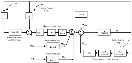
Figure 2.
Studied MG model.
2.2. Structure of VIC Loop
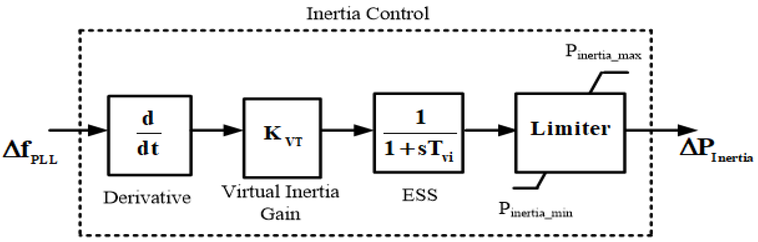
Low inertia MGs are susceptible to frequency instability with fewer rotating machines [31]. The main aim of the VIC is to provide virtual inertia support to the studied MG to improve frequency regulation and in this manner permits a high portion of RESs penetration inside the micro grid. Here, the derivative control method is applied to assess the change in frequency which can change the ESS active power to a set point after certain aggravation/disturbance. In this manner, the VIC is copied by utilizing the ESS and control loop given in Figure 3.
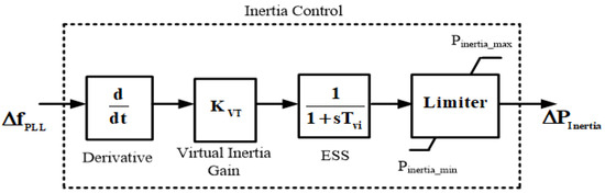
Figure 3.
Model of VIC.
To acquire the characteristics of ESS, a low-pass filter is employed to remove the noise problem. A limiter is present to limit the power output limit. The control law for the VIV loop can be stated as [28]:
where KVI, TVI and ΔfPLL are the control gain, VIC time constant and the frequency variation (output of PLL), respectively.
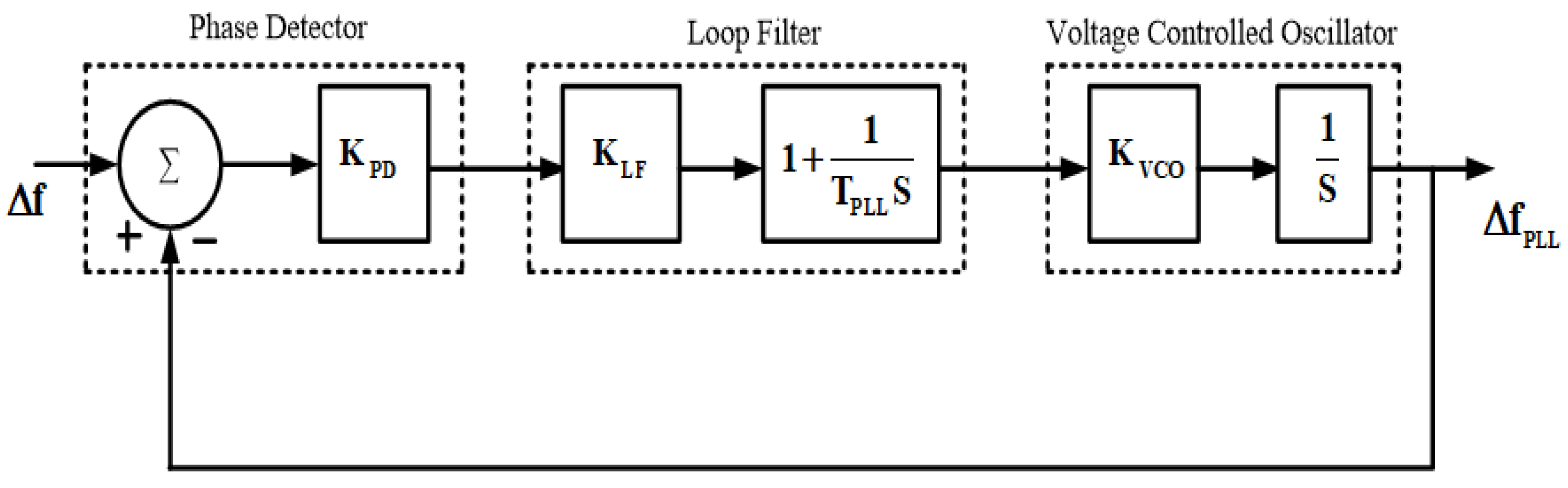
In this manner, the capacity of VIC to respond to the rapid frequency variations depends on PLL. Figure 4, displays the structure of PLL, which predominantly contains a voltage-controlled oscillator, a filter and a phase detector.
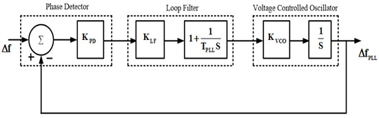
Figure 4.
PLL structure details.
3. Proposed Controller Structure and the Problem Formulation
3.1. Structure of AFPIDF Controller
Traditional PID structures are simple, effective, and easy to implement [32,33]. Nevertheless, the performance of PID degrades in the presence of nonlinearities and constraints. On the other hand, fuzzy logic is flexible and easy to understand and implement. It helps to mimic the logic of human thought. It is a highly suitable method for uncertain or approximate reasoning; therefore, the performance can be enhanced by employing a fuzzy PID (FPID) controller. However, in the case of the FPID controller, the input signal is passed through the FLC to obtain the desired output. To take the benefits of both the PID and FPID controller, an adaptive type of FPID with a derivative filter (AFPIDF) is proposed in the current study, as revealed in Figure 5. Frequency deviation (∆f) is considered as an error. The introduced controller has five parameters, two input scaling factors (K1, K2) and the PID controller parameters (KP, KI, KD) that must be selected accurately to obtain the desired frequency regulation.
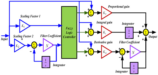
Figure 5.
Proposed AFPIDF controller.
3.2. Objective Function
To minimize ∆F of the studied MG, an integral criterion with the objective to minimize the ∆F, as well as control actions, is taken as the objective function as:
where t is the simulation time, is the controller output. In the above Equation, weights and are assigned values of 10 and 100, respectively, to make both the components in Equation (2) competitive during search procedure.
To find the AFPIDF controller parameters, a problem of optimization is formed as:
Minimize J
Subject to
where i = 1, 2, P, I & D (the two scaling factors and PID parameters), the subscripts Min and Max represent the lower and upper bounds of the gains and taken in the range (0–2).
There filter coefficient N is taken as 100.
4. Proposed Modified GJO Algorithm
4.1. Golden Jackal Optimization (GJO) Algorithm
The Golden Jackal Optimization (GJO) algorithm is motivated by the collective hunting activities of golden jackals. The basic steps of GJO are prey probing, encircling, and attacking, which are followed in GJO. The steps of the GJO procedure are [28].
4.1.1. Search Space Design
The GJO is a population-based technique, where the starting positions are randomly located over the search area as:
where Xmax and Xmin are the bound for variables and “Rn” is a random value from 0 to 1.
This step generates the starting matrix Prey is given in Equation (6), out of which the two fittest is taken as jackal pair.
where Xij represents the j-th element of i-th prey. There is “n” no. of preys with “v” variables. The prey location represents a definite solution. An objective function is used to find the fitness of each prey in the optimization process. The fitness of all preys (FPrey) is given by:
where “f” is the objective function. The two fittest are called Male Jackal and Female Jackal.
4.1.2. Exploration Phase
Jackals know how to identify and trail the prey, but occasionally the prey are not trapped simply and escape. Later, the jackals pause and hunt for other prey. Hunting is led by the male jackal followed by the female jackal as:
where, “t” represent the present, Prey(t) is the location of the prey in t, and XM(t) and XFM(t) represent the positions in t &X1(t) and X2(t) are new locations of the male and female jackal, respectively.
E is escaping prey energy found as:
E1 and E0 represent the declining and initial energy of the prey. E0 is varied from −1 to 1 and found as:
where “r” is a random value from 0 and 1. E1 is found as:
where c1 equals to 1.5, E1 is gradually reduced from 1.5 to 0 during iterations.
The value of in Equations (8) and (9) calculates the distance between preyand jackal, which is deducted or added to the present location of the jackal based on E. “rl” is an arbitrary value determined based on Levy Flight (LF) distribution as in Equation (13).
The LF is calculated by:
where u, v are arbitrary parameters in the range (0, 1), β is a constant and taken as 1.5. The jackal locations are reorganized as:
4.1.3. Exploitation Phase
Once the prey is confronted by jackals its energy declines and then the jackals encircles the prey identified in the earlier phase. Thereafter, they jump on prey and eat it. This action of jackal’s collected pursuing is expressed as:
The purpose of “rl” in Equations (16) and (17) is to offer random actions in the exploitation phase, supporting exploration and local optima evasion.
4.1.4. Moving from Exploration to Exploitation
In the GJO procedure, E value is used in moving from exploration to exploitation. The prey’s energy declines significantly throughout evading behavior. When E0 diminishes from 0 to −1, the prey is actually weakening, and when E0 increases from 0 to 1, the strength of the prey increases. If |E| > 1, the jackal pairs search diverse segments for exploring prey, and if |E| < 1, jackals assault the prey and carries out exploitation.
4.2. Modified GJO (mGJO) Algorithm
The problem associated with the GJO algorithm is the identification of the best locations of Jackals at the initial stages. Therefore, increasing the step size in the beginning phase of the algorithm may result in deviating the Jackal’s locations from the ideal locations. Thus, to control the movement of Jackals in the early stages, sine cosine adopted scaling factors (SCaSF) can be utilized. Inclusion of SCaSF, modifies the Jackal’s location, thus improving the search capability of the calculation. For proper exploitation of the search space, the algorithm should be able to find better positions and for the exploration, the solution is equipped to search beyond and also among the best locations of Jackal’s found in the previous iterations. The cyclic shape of sine and cosine functions enables a solution to be repositioned nearby another solution. The said procedure can ensure improved exploitation and exploration ability of the original GJO.
The scaled positions of Jackals in the proposed mGJO are modified as:
where ScaSF is determined as:
where RD is a random value in the range [0, 1] and WT1&WT2are weighting factors. For the proper determination of weights WT1 &WT2, various values of weights are tested. It is observed that the best results are acquired when WT1&WT2are chosen as 10 &9, respectively.
5. Simulation Results and Discussion
5.1. Benchmark Functions Testing
Initially, the effectiveness of the suggested mGJO technique is verified by taking some unimodal and multimodal functions, as shown in Table 1 [28]. To validate the benefit of the mGJO strategy, outcomes of the mGJO are equated with GJO, GWO, GSA, PSO, TLBO and ALO results, as carried out in the original paper, taking the same algorithm parameters [28]. For all the methods, search agents and iterations are taken as 30 and 200, respectively, as carried out in [28] for a fair comparison. The measurable results, such asbest, average, worst and standard deviation for 30 runs are assembled in Table 2, from which it is noticed that proposed mGJO out performs other algorithms for almost all test functions.

Table 1.
Benchmark functions.
Table 2.
Results for benchmark functions.
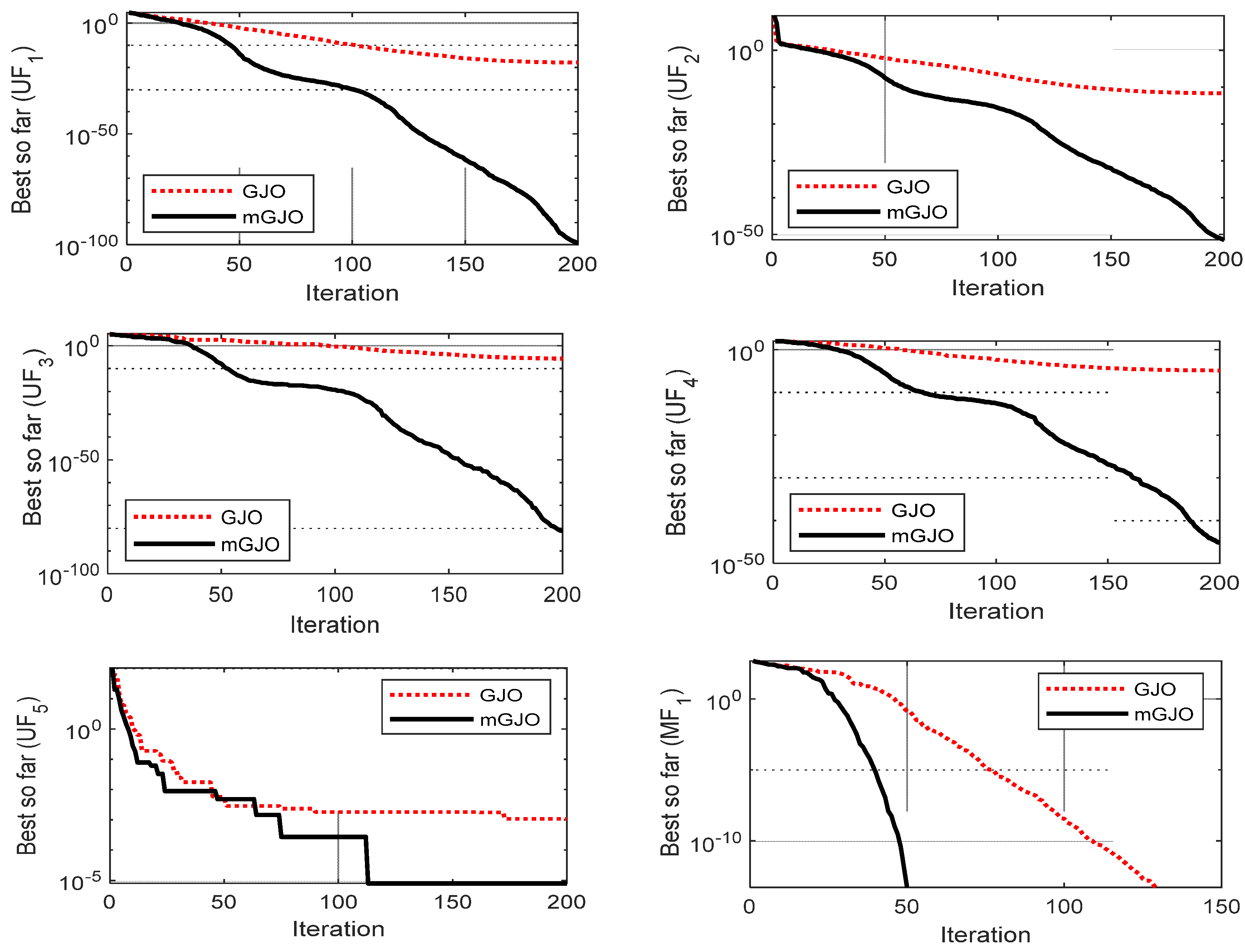
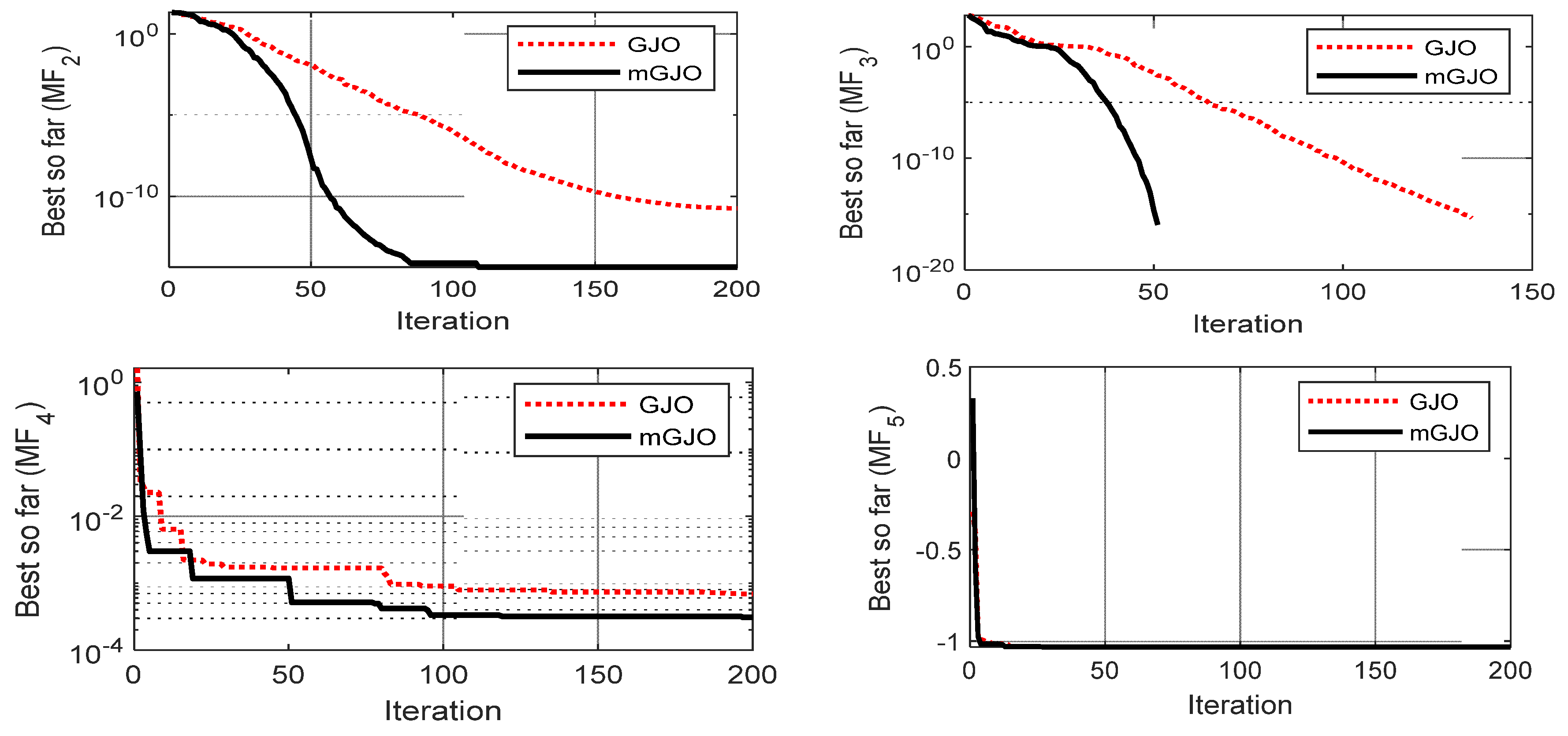
The superior convergence characteristic of GJO over GWO, GSA, PSO, TLBO and ALO has been demonstrated in reference [28]. Here, the convergence characteristic of mGJO is compared with the original GJO and shown in Figure 6, which clearly demonstrates the superior convergence characteristic of mGJO over GJO.
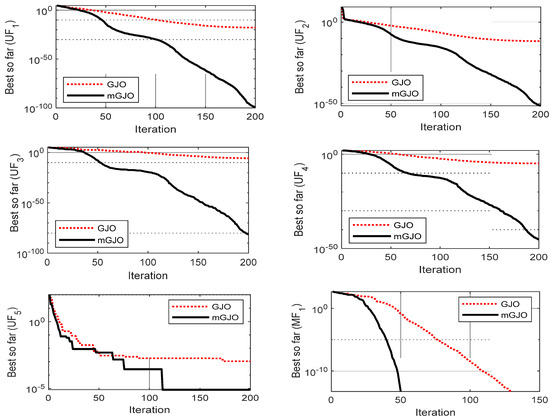
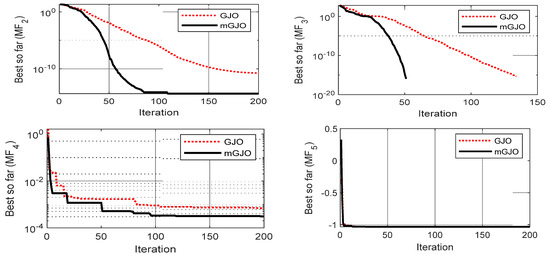
Figure 6.
Convergence curves (mGJO Vs GJO).
In many applications, conventional optimization techniques have been applied to solve engineering design problems. For example, in [34], a self-feedback recurrent fuzzy neural network estimator for an active power filter has been proposed to improve harmonic compensation of the performance of where a gradient descent optimization technique has been applied to solve the optimal control problem. A Gradient Based Optimizer (GBO) method has been applied to solve the Unit Commitment problem [35] and to identify the best parameters of PEM fuel cell [36]. In these types of applications, the proposed mGJO method can be applied to obtain the improved result.
5.2. Implementation of mGJO in Engineering Design Problem
In the next stage, the mGJO is applied to the engineering design problem, i.e., controller design for frequency regulation of the MG system, shown in Figure 1. The model of the system under study is developed in a MATLAB/SIMULINK environment, where the controller parameters are the search variables. The optimization routines are written in a separate m file. The model is simulated by applying a disturbance; the objective function values are calculated and transferred to the optimization routine through workspace. At the end of the optimization routine, the best controller parameters corresponding to the minimum value of objective function are obtained.
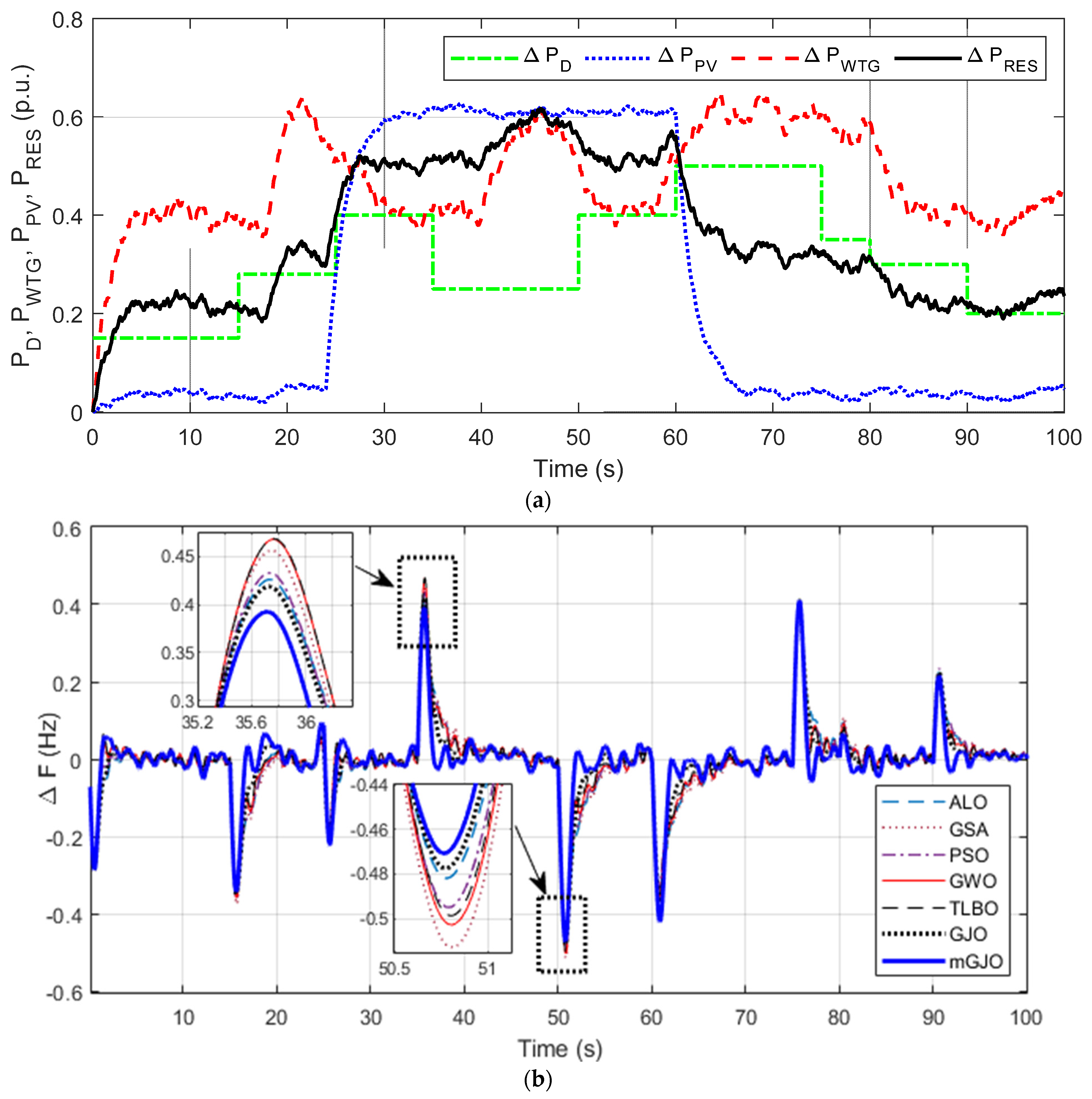
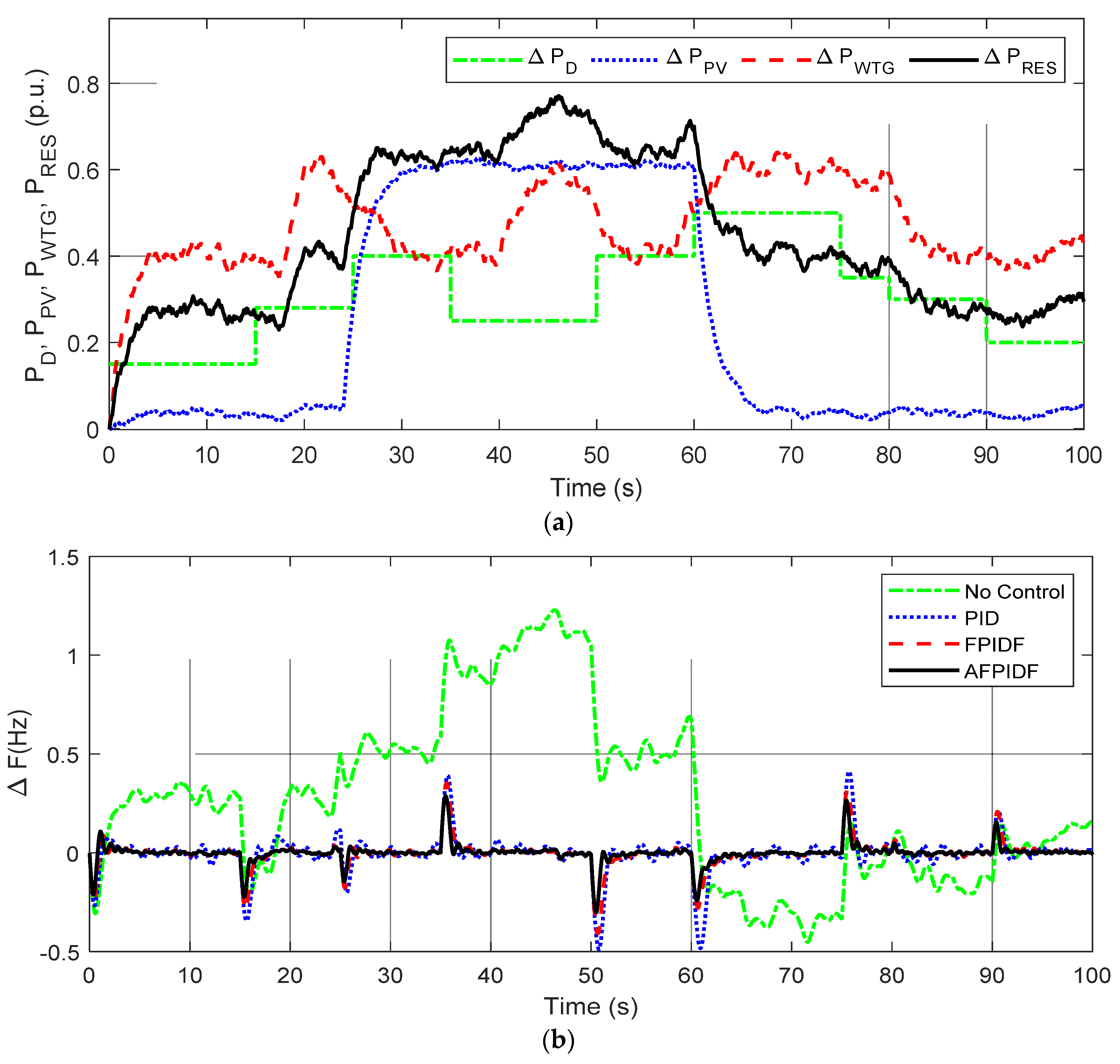
The variations in load demand (ΔPD), wind power (ΔPWTG), solar power (ΔPPV), and the total renewable sources (ΔPRES) are shown in Figure 7a. To authenticate the better performance of the mGJO method, firstly, PID controllers are assumed and PID parameters (KP, KI, KD)optimized by the mGJO, GJO, GWO, GSA, PSO, TLBO and ALO techniques. All the techniques are run 30 times independently and the best parameters as per minimum J value given by Equation (2) obtained are chosen, shown in Table 3. It is clear from Table 3 that a smaller amount of J value is attained with GJO compared to GWO, GSA, PSO, TLBO and ALO techniques. The J value is further reduced when mGJO is used. The % decrease in J value with the proposed mGJO technique compared to GJO, GWO, GSA, PSO, TLBO and ALO techniques are 14.68%, 15.34%, 18.36%, 23.66%, 24.21%, and 24.85%, respectively.
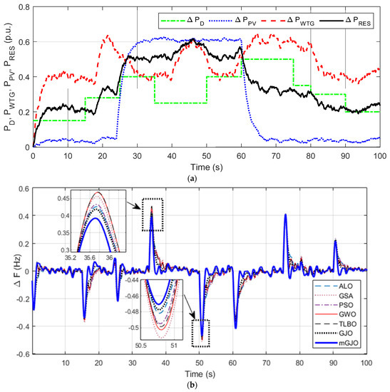
Figure 7.
(a) Variation in ΔPD, ΔPWTG, ΔPPV, ΔPRES, (b) System response with PID.
Table 3.
Optimized controller values.
The comparative ∆F responses for different techniques (with PID) is shown in Figure 7b. It is observed from Figure 7b that, the response with the mGJO technique is superior to GJO, GWO, GSA, PSO, TLBO and ALO techniques. The comparison report of transient characteristics using integral errors and Maximum Overshoot (MOs)/Maximum Undershoot (MUs) of Figure 7b are given in Table 4. It is observed from Table 4 that the numerical value integral errors, MOs/Mus, due to the mGJO optimized PID controller, are found to be least compared, the same with the GJO, GWO, GSA, PSO, TLBO and ALO optimized PID controller. This confirms the superiority of the mGJO technique over the GJO, GWO, GSA, PSO, TLBO and ALO techniques in the studied controller design problem.
Table 4.
Performance with PID tuned by different techniques.
In the next stage, the mGJO technique is employed to optimize the proposed AFPIDF and FPID controllers. The structure of FPID is similar to the AFPIDF shown in Figure 3, without the direct link from input to output. The optimized values are given in Table 3, from which it is clear that least J value is attained with AFPIDF compared to FPID and PID. The % decrease improvement in J values using AFPIDF compared to FPID and PID are 42.93% and 68.54%, respectively.
To evaluate the effect of RESs integration level on the MG, the following conditions are considered
5.2.1. Condition 1: Normal RES Integration
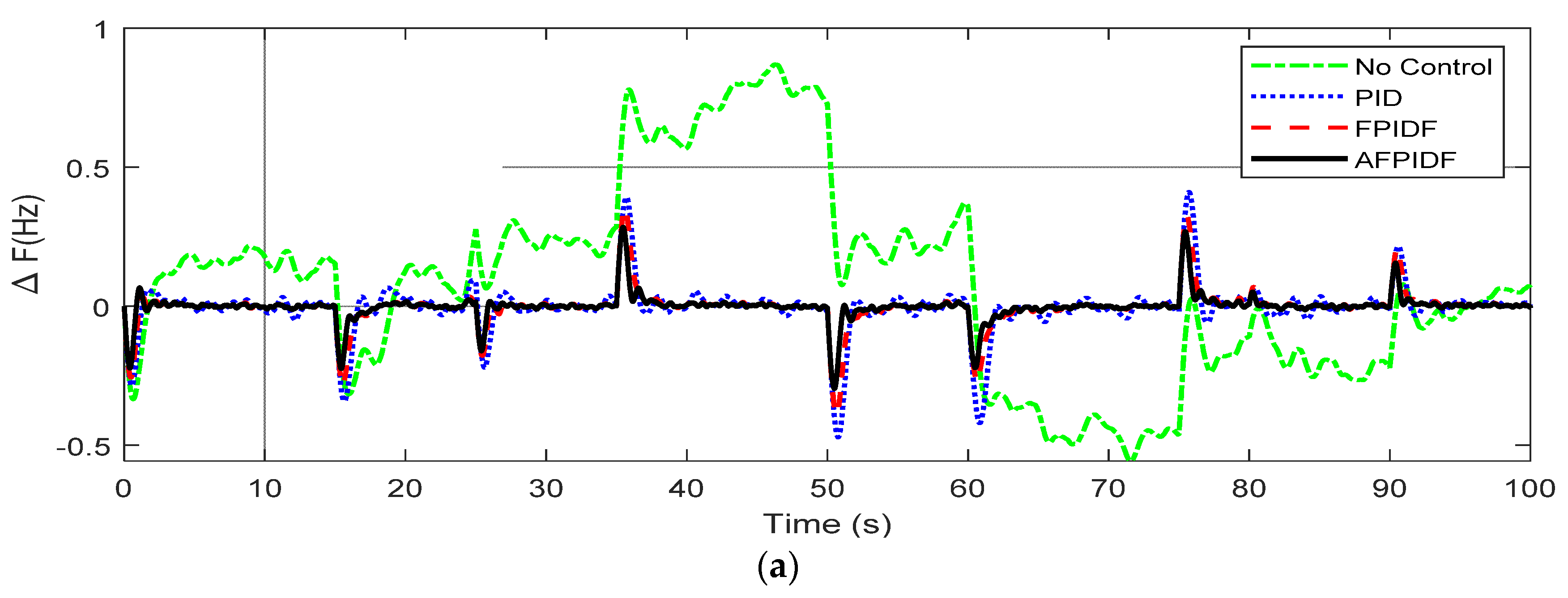
In this condition, normal (100%) RESs integration is assumed, and uncontrolled variations are shown in Figure 7a. Figure 8a reveals the ∆F response of the MG. It can be noticed from Figure 8a that the transient performance without control is highly oscillatory, with large deviations in system frequency. The response with AFPIDF is superior to FPID and PID with lesser integral and MOs/MUs than other controllers. Figure 8b displays the power output of the thermal unit (ΔPTh) and inertia (ΔPInertia) power for the above case. In Figure 8b, negative values indicate a decrease in respective power. It can be seen from Figure 8b that when ΔPRES increases, the ΔPTh and ΔPInertia values decrease.
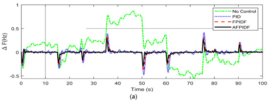
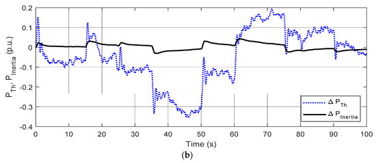
Figure 8.
Response for Condition-1 (a) ΔF (b) ΔPTh, ΔPInertia.
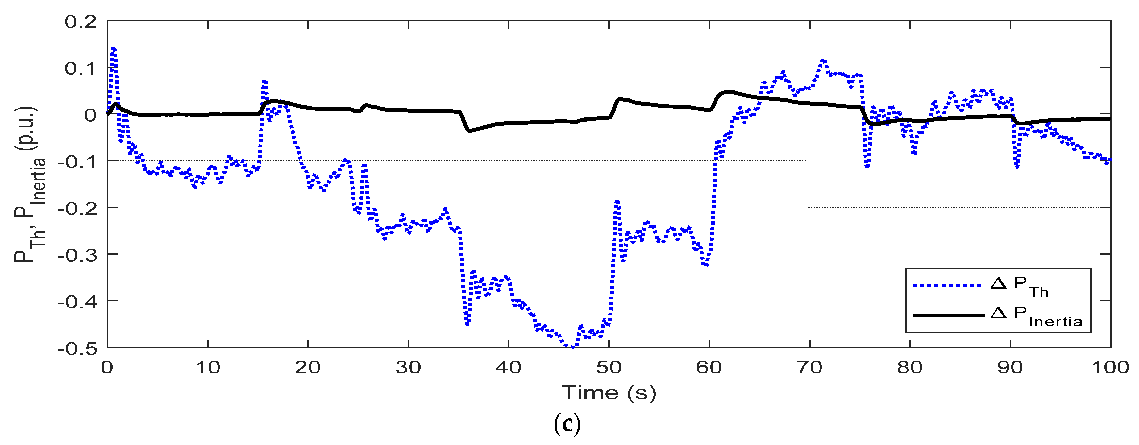
5.2.2. Condition 2: Reduced RES Integration
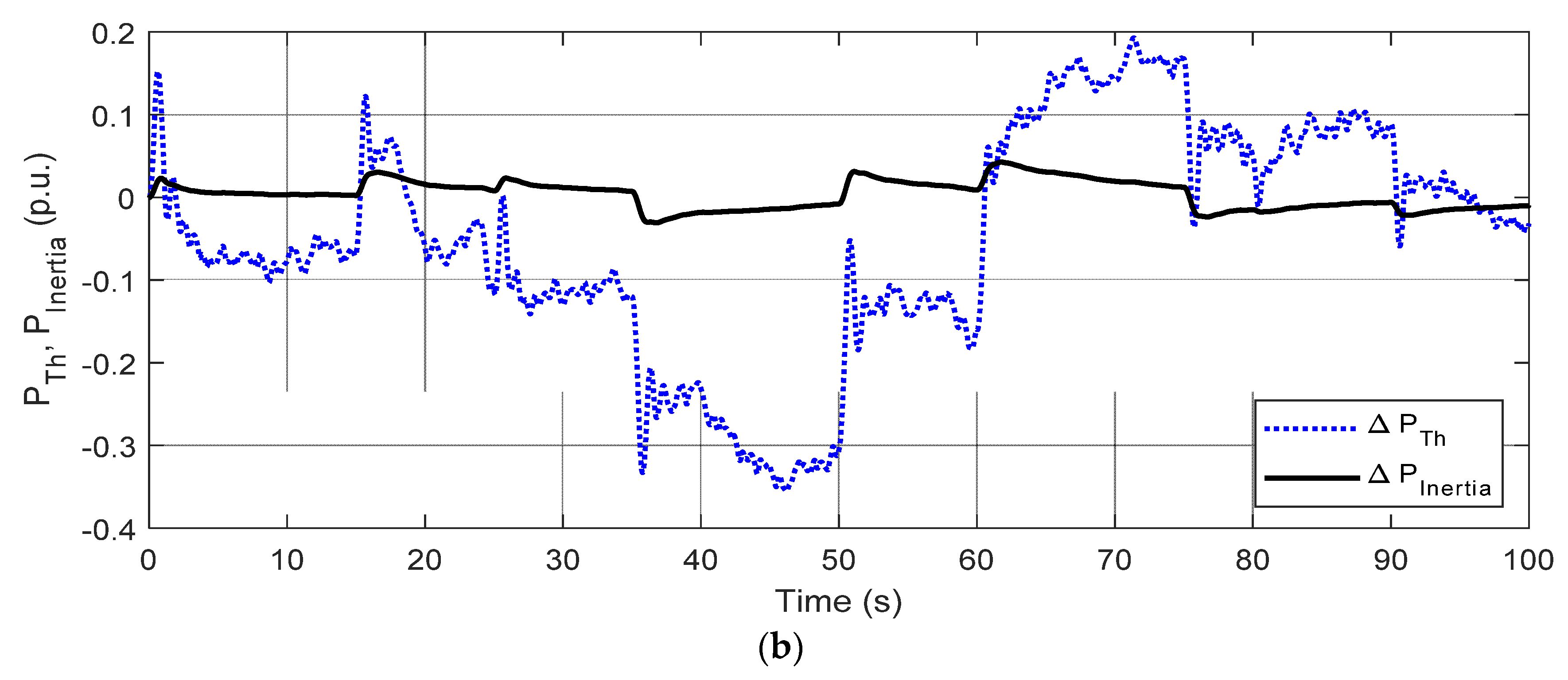
In this condition, the RESs integration level is reduced to half, i.e., 50% of its normal values, as revealed in Figure 9a, and the ∆F response in displayed in Figure 9b. In this case, it is also seen that the response with AFPIDF is superior to FPID and PID controllers. The response of ΔPTh and ΔPInertia is shown in Figure 9c. It can be seen from Figure 9a,c that when the penetration level of ΔPRES decreases, the ΔPTh and ΔPInertia values increase.

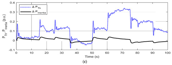
Figure 9.
Response for Condition-2 (a) ΔPD, ΔPWTG, ΔPPV, ΔPRES (b) ΔF (c) ΔPTh, ΔPInertia.
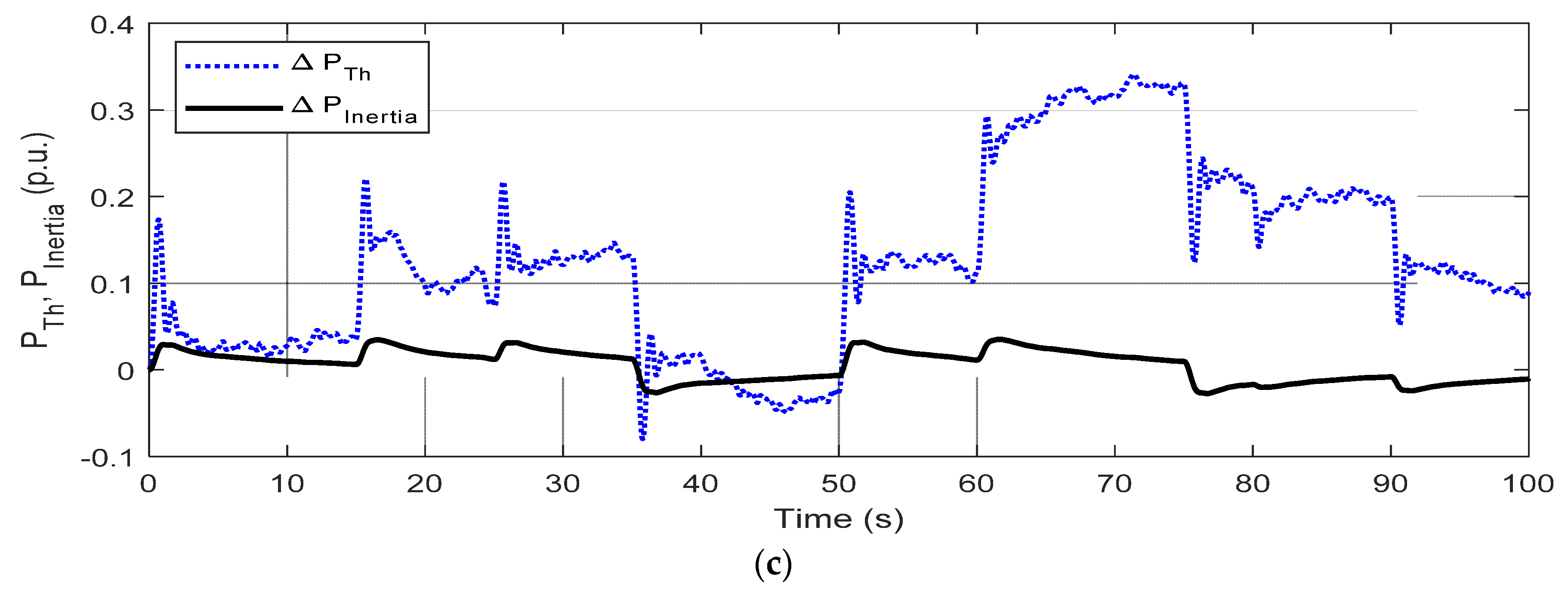
5.2.3. Condition 3: Increased RES Integration
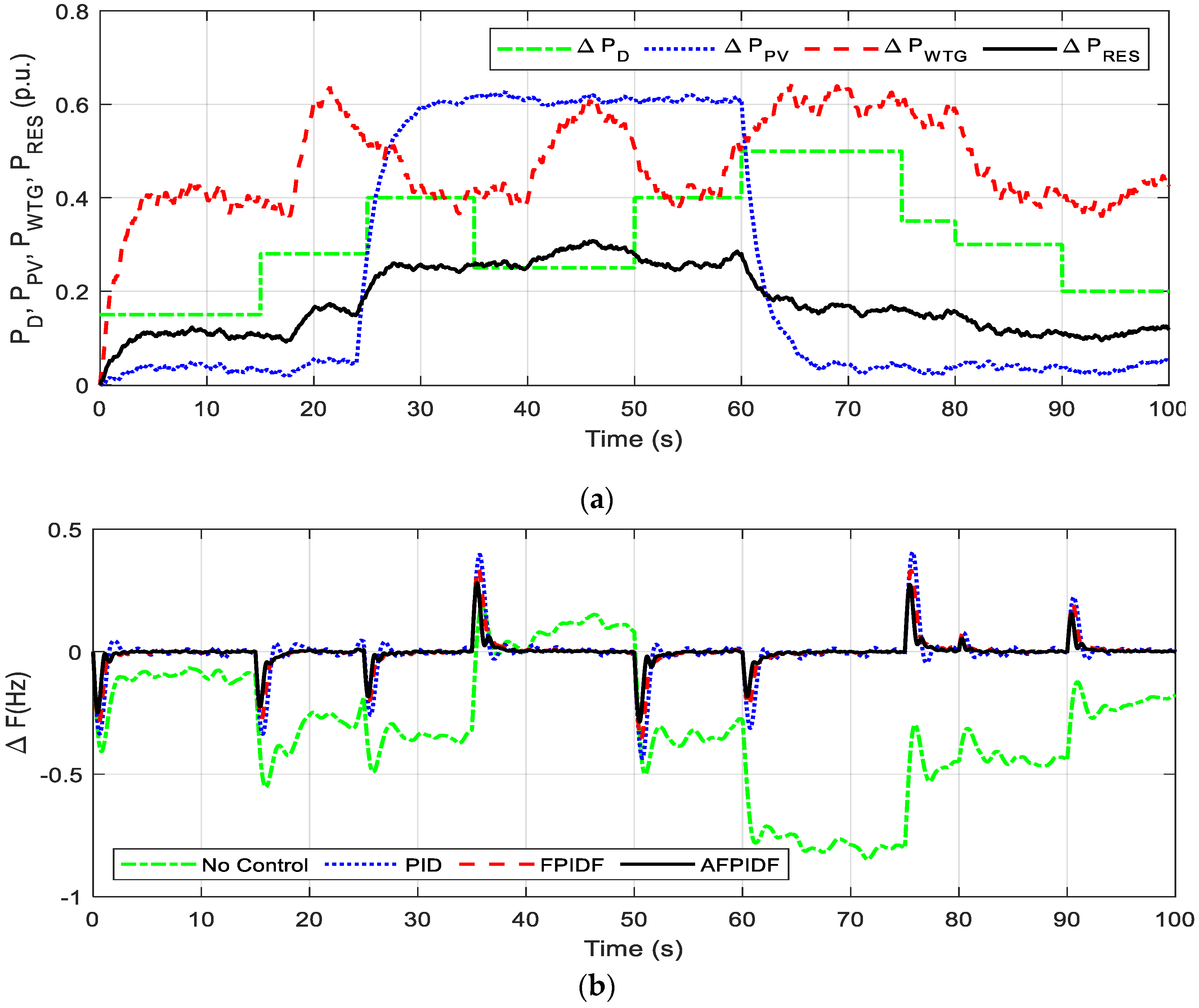
In this case, the penetration level of ΔPRES is increased to 125% as presented in Figure 10a and the ∆F response is shown in Figure 10b. Improved system responses are obtained with AFPIDF is superior to FPID and PID controllers. The response of ΔPTh and ΔPInertia are shown in in Figure 10c, from which it is clear that as the penetration level of ΔPRES increases, ΔPTh and ΔPInertia values are suitably changed to minimize the frequency deviation.
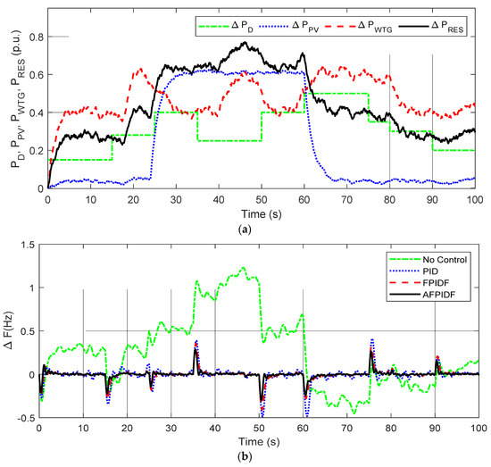
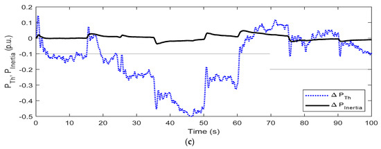
Figure 10.
Response for Condition-2 (a) ΔPD, ΔPWTG, ΔPPV, ΔPRES (b) ΔF (c) ΔPTh, ΔPInertia.
The comparison report of the transient characteristics of various values integral errors, MOs/MUs, of ΔF for all the conditions are given in Table 5. It is observed from this table that the numerical values of integral errors, MOs and Mus, due to AFPIDF, are found to be least compared to other approaches.
Table 5.
Performance index comparison of different control approaches for all cases.
6. Conclusions
This study addresses the frequency regulation issue of a MG by employing an mGJO based AFPIDF controller with VIC. Initially, the dominance of the mGJO over GJO, GWO, GSA, PSO, TLBO and ALO is demonstrated by taking a set of benchmark functions. The proposed mGJO technique is then employed to design a PID controller for frequency regulation of an islanded MG in the VIC environment. It is observed that with the same controller structure, the % decrease in J value with suggested mGJO related to GJO, GWO, GSA, PSO, TLBO and ALO techniques are 14.68%, 15.34%, 18.36%, 23.66% 24.21%, and 24.85%, respectively. In the next stage, the proposed mGJO method is utilized to tune AFPID and PFPID controllers and it is observed that % decrease in J value with AFPIDF related to FPID and PID are 42.93% and 68.54%, respectively. It is further noticed that the proposed mGJO optimized AFPIDF approach for frequency control performs satisfactorily with various levels of asymmetric RES penetration. In the current study, a fixed virtual inertia constant is considered. For future work, an adaptive virtual inertia control system using fuzzy logic can be developed. Additionally, VIC control for multi-area systems can be considered.
Author Contributions
Conceptualization, Methodology, Supervision, N.K.M.; Formal analysis, Validation, Writing, S.N.K. All authors have read and agreed to the published version of the manuscript.
Funding
This research received no external funding.
Institutional Review Board Statement
Not applicable.
Informed Consent Statement
Not applicable.
Data Availability Statement
Not applicable.
Conflicts of Interest
The authors declare no conflict of interest.
Appendix A
Governor time constant (Tg) = 0.1 s, Turbine time constant (Tt) = 0.4 s, Virtual inertia time constant (TVI) = 0.4 s, Frequency bias factor (β) = 1 p.u.MW/Hz; Droop characteristic (R) = 2.4 Hz/p.u.MW; System damping (D) = 0.015 p.u.MW/Hz, System inertia constant (H) = 0.083 p.u.MW s; Wind turbine time constant (TWT) = 1.5 s, Solar system time constant (TPV) = 1.85 s, Gate valve limits (VU/VL) = ±0.5, ESS capacity (PINTERTIA) = ±0.25, Virtual inertia gain (KVT) = 0.8; Phase detector gain (KPD) = 1.0; Loop filter gain (KLF) = 1.0; Voltage oscillator gain (KVCO) = 1.0; Time constant of PLL (TPLL) = 1.5 s.
References
- Pogaku, N.; Prodanovic, M.; Green, T.C. Modeling, analysis and testing of autonomous operation of an inverter-based microgrid. IEEE Trans. Power Electron. 2007, 22, 613–625. [Google Scholar] [CrossRef]
- Debrabandere, K.; Bolsens, B.; Van den Keybus, J.; Woyte, A.; Driesen, J.; Belmans, R. A voltage and frequency droop control method for parallel inverters. IEEE Trans. Power Electron. 2007, 22, 1107–1115. [Google Scholar] [CrossRef]
- Alsiraji, H.A.; El-Shatshat, R. Comprehensive assessment of virtual synchronous machine based voltage source converter controllers. IET Gen. Trans. Distribn. 2017, 11, 1762–1769. [Google Scholar] [CrossRef]
- Liu, J.; Miura, Y.; Bevrani, H.; Ise, T. Enhanced Virtual Synchronous Generator Control for Parallel Inverters in Microgrids. IEEE Trans. Smart Grid 2017, 8, 2268–2277. [Google Scholar] [CrossRef]
- Im, W.S.; Wang, C.; Liu, W.; Liu, L.; Kim, J.M. Distributed virtual inertia based control of multiple photovoltaic systems in autonomous microgrid. IEEE/CAA J. Autom. Sin. 2017, 4, 512–519. [Google Scholar]
- Ma, Y.; Cao, W.; Yang, L.; Wang, F.; Tolbert, L.M. Virtual synchronous generator control of full converter wind turbines with short-term energy storage. IEEE Trans. Ind. Electn. 2017, 64, 8821–8831. [Google Scholar] [CrossRef]
- Torres, M.A.L.; Lopes, L.A.C.; Morán, L.A.T.; Espinoza, J.R.C. Self-tuning virtual synchronous machine: A control strategy for energy storage systems to support dynamic frequency control. IEEE Trans. Energy Conv. 2014, 29, 833–840. [Google Scholar] [CrossRef]
- Soni, N.; Doolla, S.; Chandorkar, M.C. Improvement of transient response in microgrids using virtual inertia. IEEE Trans. Power Del. 2013, 28, 1830–1838. [Google Scholar] [CrossRef]
- Andalib-Bin-Karim, C.; Liang, X.; Zhang, H. Fuzzy-secondary-controller-based virtual synchronous generator control scheme for interfacing inverters of renewable distributed generation in microgrids. IEEE Trans. Ind. Appln. 2018, 54, 1047–1061. [Google Scholar] [CrossRef]
- Fang, J.; Li, H.; Tang, Y.; Blaabjerg, F. Distributed power system virtual inertia implemented by grid-connected power converters. IEEE Trans. Power Electn. 2018, 33, 8488–8499. [Google Scholar] [CrossRef]
- D’Arco, S.; Suul, J.A.; Fosso, O.B. A virtual synchronous machine implementation for distributed control of power converters in smartgrids. Electr. Power Syst. Res. 2015, 122, 180–197. [Google Scholar] [CrossRef]
- Hirase, Y.; Abe, K.; Sugimoto, K.; Shindo, Y. A grid-connected inverter with virtual synchronous generator model of algebraic type. Elect. Eng. Jpn. 2013, 184, 10–21. [Google Scholar] [CrossRef]
- Kerdphol, T.; Watanabe, M.; Hongesombut, K.; Mitani, Y. Self-adaptive virtual inertia control-based fuzzy logic to improve frequency stability of microgrid with high renewable penetration. IEEE Access 2019, 7, 76071–76083. [Google Scholar] [CrossRef]
- Kerdphol, T.; Rahman, F.S.; Mitani, Y.; Watanabe, M.; Küfeoglu, S.K. Robust virtual inertia control of an islanded microgrid considering high penetration of renewable energy. IEEE Access 2017, 6, 625–636. [Google Scholar] [CrossRef]
- Ali, H.; Magdy, G.; Li, B.; Shabib, G.; Elbaset, A.A.; Xu, D.; Mitani, Y. A new frequency control strategy in an islanded microgrid using virtual inertia control-based coefficient diagram method. IEEE Access 2019, 7, 16979–16990. [Google Scholar] [CrossRef]
- Sockeel, N.; Gafford, J.; Papari, B.; Mazzola, M. Virtual inertia emulator-based model predictive control for grid frequency regulation considering high penetration of inverter-based energy storage system. IEEE Trans. Sustain. Energy 2020, 11, 2932–2939. [Google Scholar] [CrossRef]
- Saleh, A.; Omran, W.A.; Hasanien, H.M.; Tostado-Vrliz, M.; Alkuhayli, A.; Jurado, F. Manta ray foraging optimization for the virtual inertia control of islanded microgrids including renewable energy sources. Sustainability 2022, 14, 4189. [Google Scholar] [CrossRef]
- Fu, S.; Sun, Y.; Liu, Z.; Hou, X.; Han, H. Power oscillation suppression in multi-VSG grid with adaptive virtual inertia. Int. J. Elect. Power Energy Syst. 2022, 135, 107472. [Google Scholar] [CrossRef]
- Khazali, A.; Rezaei, N.; Saboori, H.; Guerrero, J.M. Using PV systems and parking lots to provide virtual inertia and frequency regulation provision in low inertia grids. Elect. Power Syst. Res. 2022, 207, 107859. [Google Scholar] [CrossRef]
- Abubakr, H.; Mohamed, T.H.; Hussein, M.M.; Guerrero, J.M.; Agundis-Tinajero, G. Adaptive frequency regulation strategy in multi-area microgrids including renewable energy and electric vehicles supported by virtual inertia. Int. J. Elect. Power Energy Syst. 2021, 129, 106814. [Google Scholar] [CrossRef]
- Ratnam, K.S.; Palanisamy, K.; Yang, G. Future low-inertia power systems: Requirements, issues, and solutions—A review. Renew. Sustain. Energy Rev. 2020, 124, 109773. [Google Scholar] [CrossRef]
- Makolo, P.; Oladeii, I.; Zamora, R.; Lie, T.T. Short-range inertia prediction for power networks with penetration of RES, TENCON 2021. In Proceedings of the 2021 IEEE Region 10 Conference (TENCON), Auckland, New Zealand, 7–10 December 2021. [Google Scholar]
- Carlini, E.M.; Del Pizzo, F.; Giannuzzi, G.M.; Lauria, D.; Mottola, F.; Pisani, C. Online analysis and prediction of the inertia in power systems with renewable power generation based on a minimum variance harmonic finite impulse response filter. Int. J. Elect. Power Energy Syst. 2021, 131, 107042. [Google Scholar] [CrossRef]
- Magdy, G.; Shabib, G.; Elbaset, A.A.; Mitani, Y. A novel coordination scheme of virtual inertia control and digital protection for microgrid dynamic security considering high renewable energy penetration. IET Renew. Power Gener. 2019, 13, 462–474. [Google Scholar] [CrossRef]
- Mandal, R.; Chatterjee, K. Virtual inertia emulation and RoCoF control of a microgrid with high renewable power penetration. Electr. Power Syst. Res. 2021, 194, 107093. [Google Scholar] [CrossRef]
- Othman, A.M.; El-Fergany, A.A. Adaptive virtual-inertia control and chicken swarm optimizer for frequency stability in power grids penetrated by renewable energy sources. Neural Comput. Appl. 2021, 33, 2905–2918. [Google Scholar] [CrossRef]
- Khadangaa, R.K.; Das, D.; Kumar, A.; Panda, S. An improved parasitism predation algorithm for frequency regulation of a virtual inertia control based AC microgrid. Energy Sources Part A Rec. Utilz. Env. Effects 2022, 44, 1660–1677. [Google Scholar] [CrossRef]
- Chopra, N.; Ansari, M.M. Golden jackal optimization: A novel nature-inspired optimizer for engineering applications. Expert Syst. Appln. 2022, 198, 116924. [Google Scholar] [CrossRef]
- Mishra, S.; Nayak, P.C.; Prusty, R.C.; Panda, S. Modified multiverse optimizer technique-based two degree of freedom fuzzy PID controller for frequency control of microgrid systems with hydrogen aqua electrolyzer fuel cell unit. Neural Comput. Appln. 2022. [Google Scholar] [CrossRef]
- Mishra, S.; Nayak, P.C.; Prusty, R.C.; Panda, S. Novel load frequency control scheme for hybrid power systems employing interline power flow controller and redox flow battery. Energy Sources Part A Rec. Utilz. Env. Effects 2022. [Google Scholar] [CrossRef]
- Kerdphol, T.; Rahman, F.S.; Watanabe, M.; Mitani, Y. Robust virtual inertia control of a low inertia microgrid considering frequency measurement effects. IEEE Access 2019, 7, 57550–57560. [Google Scholar] [CrossRef]
- Civelek, Z.; Cam, E.; Luy, M.; Mamur, H. Proportional-integral-derivative parameter optimization of blade pitch controller in wind turbines by a new intelligent genetic algorithm. IET Renew. Pow. Gen. 2016, 10, 1220–1228. [Google Scholar] [CrossRef]
- Ho, W.K.; Hang, C.C.; Cao, L.S. Tuning of PID controllers based on gain and phase margin specifications. Automatica 1995, 31, 497–502. [Google Scholar] [CrossRef]
- Fei, J.; Liu, L. Real-time nonlinear model predictive control of active power filter using self-feedback recurrent fuzzy neural network estimator. IEEE Trans. Ind. Electn. 2022, 69, 8366–8376. [Google Scholar] [CrossRef]
- Said, M.; Houssein, E.H.; Deb, S.; Alhussan, A.A.; Ghoniem, R.M. A novel gradient based optimizer for solving unit commitment problem. IEEE Access 2022, 10, 18081–18092. [Google Scholar] [CrossRef]
- Rezk, H.; Ferahtia, S.; Djeroui, A.; Chouder, A.; Houari, A.; Machmoum, M.; Abdelkareem, M. Optimal parameter estimation strategy of PEM fuel cell using gradient-based optimizer. Energy 2022, 239, 122096. [Google Scholar] [CrossRef]


Publisher’s Note: MDPI stays neutral with regard to jurisdictional claims in published maps and institutional affiliations. |
© 2022 by the authors. Licensee MDPI, Basel, Switzerland. This article is an open access article distributed under the terms and conditions of the Creative Commons Attribution (CC BY) license (https://creativecommons.org/licenses/by/4.0/).