Continuous and Discrete Dynamical Models of Total Nitrogen Transformation in a Constructed Wetland: Sensitivity and Bifurcation Analysis

Abstract

In this research, we study a dynamical system of total nitrogen transformation in a mangrove-filled constructed wetland. The system’s variables are the mangrove biomass concentration and total nitrogen concentration in wastewater and in soil solution. We investigate the system’s dynamics by examining the local stability of the equilibriums, simulating the phase portrait and solutions and providing time-dependent parameter sensitivity analyses. The analysis shows that the level of garbage acts as the parameter for when mangrove biomass will disappear. Both the graphs of the system solutions and the sensitivity function in the case of biomass concentration and total nitrogen concentration in soil solution versus time show symmetrical features at specific time intervals. According to the sensitivity index when reaching equilibrium, the level of garbage is the most sensitive parameter to the system. In addition, we explore the model’s discrete form by investigating the conditions for the equilibrium’s local stability and presenting bifurcation diagrams for each parameter. The symmetrical aspects are visible in the visualization of the bifurcation diagram and the solutions’ chaotic behavior.

1. Introduction

Wastewater as an environmental problem has been on the rise as a result of the global effects of urbanization, climate change, and population increase [1]. Most wastewater contains nitrogen compounds, and if the wastewater is overly polluted with nitrogen, the water will smell and be unfit for human consumption [2]. Traditional biological wastewater treatment methods still have issues that prevent them from fully meeting the new environmental standards, particularly in terms of removing nitrogen compounds, which cause eutrophication in the water and seriously jeopardizes the stability of aquatic ecosystems [3]. Meanwhile, wastewater treatment via constructed wetlands as sustainable engineered systems to reduce water pollution in many different forms is spreading throughout the world during recent years [4,5]. The constructed wetlands are viewed as a substitute for traditional treatment due to its lower energy needs, ease of use and maintenance, and superior effectiveness by having microbes consume pollution produced by industrial and agricultural activity [6,7].

Constructed wetlands are a type of nature-based solution that may effectively and methodically imitate nature and its inherent traits and functions, and they can be used for a variety of land uses, including urban, agricultural, animal, and forest land uses [1]. Constructed wetlands incorporate a variety of wetland ecosystem functions via physical and ecological features, including biomass generation, habitat provision, cooling, and water purification [8,9]. The process of purifying water involves eliminating nutrients such as nitrogen, which is mostly accomplished by bacterial activity and plant uptake [1].

One of the primary nitrogen removal mechanisms in constructed wetlands is thought to involve the processes of denitrification [10]. The addition of carbon sources such as agricultural biomass materials can increase the removal of total nitrogen and significantly enhance the quality of constructed wetlands’ effluent in order to speed up the denitrification process [11]. Agricultural biomass materials are good optional carbon media because of their superior ability to supply carbon and low cost [12]. Mangroves are one of the plants that are frequently employed in constructed wetlands to generate high-quality agricultural biomass. They are self-sustaining and have unique responses to a variety of environmental stresses [13,14]. Thus, planting mangroves is one of the natural methods that may be used in constructed wetlands to improve nitrogen removal from wastewater.

One way to observe the dynamics of nitrogen removal in a constructed wetland is by using mathematical modeling such as a dynamical system. Bunwong et al. [2] proposed a mathematical model that describes the transformation of total nitrogen in a mangrove-filled constructed wetland. The model is in the form of a system of differential equations with three compartments: total nitrogen concentration in wastewater, total nitrogen concentration in soil solution, and mangrove biomass concentration. The model assumed that the growth rate of mangrove biomass production will follow the Michaelis–Menten kinetics, which illustrate the idea of limiting nutrients, i.e., there is a causal relationship between its exhaustion and the termination of growth [15], as evidenced by some empirical studies [16,17,18]. The model also assumed that the conversion of biomass is represented by a linear yield function following the suggestion in [19,20]. The analysis of the model was performed by scaling, that is all variables were scaled by the constant input rate of total nitrogen concentration. The authors also examined the existence of Hopf bifurcation for the yield function’s parameter.

The model of Bunwong et al. [2] was used and developed in the following studies. In [21], a nonlinear mathematical model of the rhizosphere microbial degradation in wetland plants was built based on impulsive state feedback control to examine the dynamics of pollutant concentration removal in constructed wetlands. The authors in [22] proposed a mathematical model of rhizosphere microbial degradation with impulsive diffusion on nutrients, which involves organic concentrations inside and outside the rhizosphere. In [23], the growth of wetland plants was examined in relation to rhizosphere dispersal and impulse input by employing the nutrient–wetland plant interaction in reducing the pollutant concentration. In order to explain the complex degradation and movement caused by introducing helpful microorganisms into the plant rhizosphere, the authors in [24] develop a three-dimensional diffusion model of the competitive rhizosphere microbes with impulsive feedback control.

In this research, we use continuous and discrete models to investigate the dynamics of total nitrogen transformation in a mangrove-filled constructed wetland. The continuous model employs the model of Bunwong et al. [2], but with a constant yield. We performed sensitivity analysis on the model’s parameters to determine how they affect the variables. By examining the sensitivity index after reaching steady-state circumstances, we may determine which parameter is the most sensitive to the system. The discrete model is derived by discretizing the continuous model. The bifurcation diagram of each parameter is presented, and the chaotic behavior is observed.

2. Dynamics of Total Nitrogen Transformation

We followed the model developed by [2] to describe the dynamics of total nitrogen transformation in a constructed wetland. Suppose $T\left(t\right)$ is the concentration of mangrove biomass, $W\left(t\right)$ is the concentration of total nitrogen in the wastewater, and $S\left(t\right)$ is the concentration of total nitrogen in the soil solution. The dynamical model of total nitrogen transformation in the wetland is given below:

$$\left\{\begin{array}{cc}\hfill \frac{dT\left(t\right)}{dt}& =\frac{\beta S\left(t\right)T\left(t\right)}{k+S\left(t\right)}-\sigma T\left(t\right)\hfill \\ \hfill \frac{dW\left(t\right)}{dt}& =Q-(\gamma +\alpha )W\left(t\right)\hfill \\ \hfill \frac{dS\left(t\right)}{dt}& =\gamma W\left(t\right)-\frac{1}{a}\frac{\beta S\left(t\right)T\left(t\right)}{k+S\left(t\right)}-\varphi S\left(t\right)\hfill \end{array}\right.$$

(1)

where all the initial values are positive: $T\left(0\right)>0,W\left(0\right)>0,S\left(0\right)>0$. The variables are all non-negative, and the parameters are all positive. The model’s diagram is given in Figure 1. The arrows represent the movement of matter through the system, and each arrow also displays the parameterizations of these flows’ rates.

The explanation of Figure 1 is as follows. The mangroves take the total nitrogen from the source and convert it into biomass. It is supposed that a filter prevents debris from falling into the pond. The concentration of the total nitrogen input rate is a constant, denoted as Q. The loss of total nitrogen in the wastewater due to runoff or evaporation is $\alpha W$. The total nitrogen exchange rate between the wastewater and soil solution is $\gamma W$. The growth rate of the mangroves follows the Michaelis–Menten kinetics $\frac{\beta S}{k+S}$. The ratio of nutrients consumed to the biomass generated by the mangroves is represented by the yield constant a. In [2], the yield coefficient was assumed to be a linear function of S. However, in this paper, we studied the model with a constant yield. Through leaching or denitrification, the total nitrogen is lost in soil solutions at the rate $\varphi S$. The litter fall rate is $\sigma T$.

2.1. Equilibrium Points and Local Stability Analysis

We denote the equilibrium points of the system (1) by $E^{*}=(T^{*},W^{*},S^{*})$. From $\frac{dW}{dt}=0$, we obtain the equilibrium $W^{*}=\frac{Q}{\gamma +\alpha }$. Meanwhile, $\frac{dT}{dt}=0$ produces the equilibriums $S^{*}=\frac{\sigma k}{\beta -\sigma }$ (with $\beta >\sigma$) or $T^{*}=0$. From this case, we have three cases.

If $\frac{dT}{dt}=0$ happens when $T^{*}=0$ and $S^{*}\ne \frac{\sigma k}{\beta -\sigma }$, then

$$0=\frac{dS}{dt}=\gamma W-\varphi S\Rightarrow S^{*}=\frac{\gamma }{\varphi }{W}^{*}=\frac{\gamma Q}{\varphi (\gamma +\alpha )}.$$

Thus, we have

$$E_1^{*}=\left(0,\frac{Q}{\gamma +\alpha },\frac{\gamma Q}{\varphi (\gamma +\alpha )}\right).$$

(2)

If $\frac{dT}{dt}=0$ happens when $T^{*}=0$ and $S^{*}=\frac{\sigma k}{\beta -\sigma }$ simultaneously, then

$$0=\frac{dS}{dt}=\gamma W-\varphi S\Rightarrow \frac{\gamma }{\varphi }{W}^{*}=S^{*}\mathrm{or}\frac{\gamma Q}{\varphi (\gamma +\alpha )}=\frac{\sigma k}{\beta -\sigma }.$$

In this case, we obtain

$$E_2^{*}=\left(0,\frac{Q}{\gamma +\alpha },\frac{\sigma k}{\beta -\sigma }\right),$$

(3)

with $\frac{\gamma Q}{\sigma (\gamma +\alpha )}=\frac{\varphi k}{\beta -\sigma }$. This means that one of the parameters depends on the others.

If $\frac{dT}{dt}=0$ happens when $T^{*}\ne 0$ and $S^{*}=\frac{\sigma k}{\beta -\sigma }$, then

$$0=\frac{dS}{dt}=\gamma W-\frac{1}{a}\frac{\beta ST}{k+S}-\varphi S\Rightarrow T^{*}=a\left(\frac{\gamma Q}{\sigma (\gamma +\alpha )}-\frac{\varphi k}{\beta -\sigma }\right).$$

Thus, we obtain

$$E_3^{*}=\left(a\left[\frac{\gamma Q}{\sigma (\gamma +\alpha )}-\frac{\varphi k}{\beta -\sigma }\right],\frac{Q}{\gamma +\alpha },\frac{\sigma k}{\beta -\sigma }\right),$$

(4)

with the positivity conditions for the equilibrium: $\frac{\gamma Q}{\sigma (\gamma +\alpha )}>\frac{\varphi k}{\beta -\sigma }$ and $\beta >\sigma$.

To analyze the local stability of each equilibrium, first, we calculate the Jacobian matrix of the system (1) at any point $E=(T,W,S)$, which is given below:

$$J\left(E\right)=\left(\begin{array}{ccc}\frac{\beta S}{k+S}-\sigma & 0& \frac{\beta kT}{{(k+S)}^2}\\ 0& -(\gamma +\alpha )& 0\\ -\frac{\beta S}{a(k+S)}& \gamma & -\left(\frac{\beta kT}{a{(k+S)}^2}+\varphi \right)\end{array}\right)$$

(5)

The stability of each equilibrium is given by the following theorems.

Theorem 1.

$E_1^{*}$ is stable if $\sigma >\overline{\sigma }$, where $\overline{\sigma }=\frac{\beta \gamma Q}{k\varphi (\gamma +\alpha )+\gamma Q}$.

Proof. 

Let $\overline{\sigma }=\frac{\beta \gamma Q}{k\varphi (\gamma +\alpha )+\gamma Q}$. The Jacobian matrix with respect to $E_1^{*}$ is

$$J\left(E_1^{*}\right)=\left(\begin{array}{ccc}\overline{\sigma }-\sigma & 0& 0\\ 0& -(\gamma +\alpha )& 0\\ -\frac{\overline{\sigma }}{a}& \gamma & -\varphi \end{array}\right),$$

with the characteristic equation

$$\left(\overline{\sigma }-\sigma -\lambda \right)\left(-(\gamma +\alpha )-\lambda \right)\left(-\varphi -\lambda \right)=0.$$

Thus, we have ${\lambda }_1=\overline{\sigma }-\sigma$, ${\lambda }_2=-(\gamma +\alpha )$, and ${\lambda }_3=-\varphi$. It is clear that ${\lambda }_2$ and ${\lambda }_3$ are less than zero. Meanwhile, ${\lambda }_1$ will be negative if $\sigma >\overline{\sigma }$. This proves the theorem.    □

In other words, Theorem 1 says that the system can be stable with a zero concentration of mangrove biomass ($T^{*}=0$) when the level of garbage is too high ($\sigma >\overline{\sigma }$).

Theorem 2.

$E_2^{*}$ is not stable.

Proof. 

The Jacobian matrix with respect to $E_2^{*}$ is

$$J\left(E_2^{*}\right)=\left(\begin{array}{ccc}0& 0& 0\\ 0& -(\gamma +\alpha )& 0\\ -\frac{\sigma }{a}& \gamma & -\varphi \end{array}\right),$$

with the characteristic equation

$$\lambda (-(\gamma +\alpha )-\lambda )(-\varphi -\lambda )=0.$$

This means there is a zero eigenvalue, which implies that the system is not stable.    □

Theorem 3.

$E_3^{*}$ is stable.

Proof. 

The Jacobian matrix with respect to $E_3^{*}$ is

$$J\left(E_3^{*}\right)=\left(\begin{array}{ccc}0& 0& aA\\ 0& -(\gamma +\alpha )& 0\\ -\frac{\sigma }{a}& \gamma & -(A+\varphi )\end{array}\right),$$

where $A=\frac{{(\beta -\sigma )}^2}{k\beta }\left(\frac{\gamma Q}{\sigma (\gamma +\alpha )}-\frac{\varphi k}{\beta -\sigma }\right)$. The characteristic equation of $J\left(E_3^{*}\right)$ is

$${\lambda }^3+a_1{\lambda }^2+a_2\lambda +a_3=0,$$

where

$$\begin{array}{cc}\hfill a_1& =\gamma +\alpha +\varphi +A, \hfill \end{array}$$

(6)

$$\begin{array}{cc}\hfill a_2& =(\gamma +\alpha )(A+\varphi )+\sigma A,\hfill \end{array}$$

(7)

$$\begin{array}{cc}\hfill a_3& =\sigma A(\gamma +\alpha ). \hfill \end{array}$$

(8)

By the Routh–Hurwitz criterion, the equilibrium $E_3^{*}$ is stable if $a_0,a_1,a_2>0$ and $a_1{a}_2>a_0$. Note that all coefficients of the characteristic equation are positive. It can be seen that $a_1{a}_2=\left[(\gamma +\alpha )(A+\varphi )+\sigma A\right](\gamma +\alpha +\varphi +A)=(\gamma +\alpha )(A+\varphi )(\gamma +\alpha +\varphi +A)+\sigma A(\varphi +A)+\sigma A(\gamma +\alpha )>\sigma A(\gamma +\alpha )=a_0.$ Therefore, by the Routh–Hurwitz criterion, $E_3^{*}$ is stable.    □

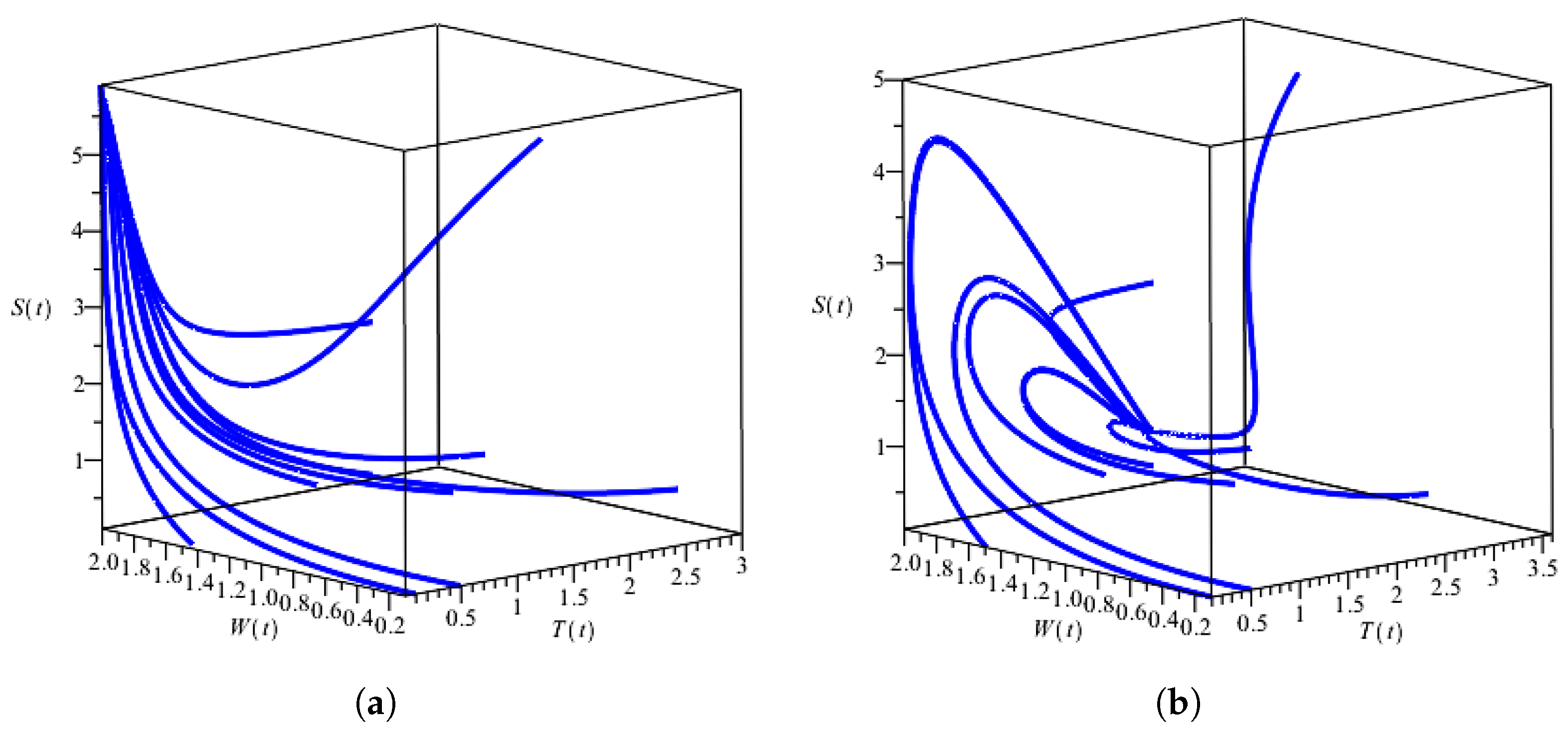
2.2. Numerical Solution

Numerical simulations of the solution of the system (1) were performed using the parameter values as presented in

Table 1. Parameter values used in the simulations.

Notation	Description	Value	Unit
$\beta$	Maximum possible value of the plant growth rate at infinite total nitrogen concentration in the soil solution	0.25	${\mathrm{time}}^{-1}$
k	Semi-saturation	1	$\left[M\right]$
$\sigma$	Level of garbage	0.1	${\mathrm{time}}^{-1}$
Q	Input level of total nitrogen concentration	1	$\left[M\right]\times {\mathrm{time}}^{-1}$
$\gamma$	Exchange rate of total nitrogen between wastewater and soil solution	0.3	${\mathrm{time}}^{-1}$
$\alpha$	Rate of total nitrogen loss in wastewater through runoff or evaporation	0.2	${\mathrm{time}}^{-1}$
a	Conversion of nutrients consumed from biomass produced	0.5	Dimensionless
$\varphi$	Rate of total nitrogen loss in the soil solution by leaching or denitrification	0.1	${\mathrm{time}}^{-1}$

. The phase portraits of the system (1) with numerous different initial values are presented in Figure 2. The solution-pairs $\left(T\right(t),W(t),S(t\left)\right)$ behave in two ways: converging to the equilibriums $E_1^{*}$ and $E_3^{*}$. The graphical solutions that converge to $E_1^{*}$ and $E_3^{*}$ are given in Figure 3. The solutions will converge to $E_1^{*}$ (the concentration of mangrove biomass is zero) if the level of garbage is too high ($\sigma >\overline{\sigma }$); otherwise, the solutions will converge to $E_3^{*}$ (positive equilibrium). Based on Table 1, then we have $\overline{\sigma }=0.2143$. In the simulations of Figure 3a,b, we used $\sigma =0.25$. In Figure 3, we can also conclude that, if the exchange rate of total nitrogen between wastewater and soil solution is bigger than the loss of total nitrogen in the soil solution ($\gamma >\varphi$), then the concentration of total nitrogen in the wastewater will converge to a value that is lower than the concentration of the total nitrogen in the soil solution. On the other hand, if $\gamma <\varphi$ (here, we used $\gamma =0.2$ and $\varphi =0.3$), then the concentration of total nitrogen in the wastewater will converge to a value that is higher than the concentration of the total nitrogen in the soil solution. Another interesting result is the appearance of symmetrical characteristics between the mangrove biomass concentration and total nitrogen concentration in the soil solution at specific intervals where the two complement each other.

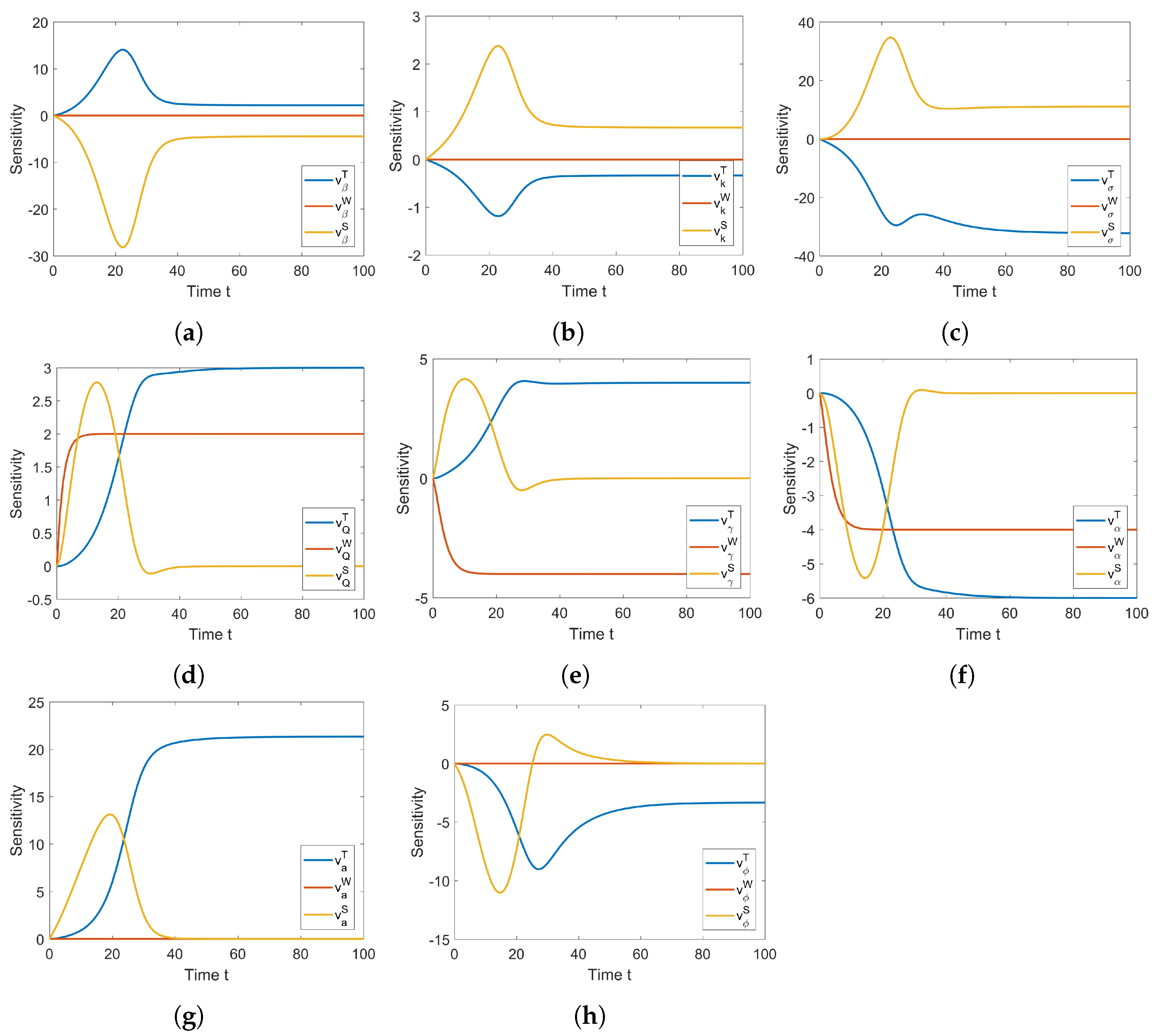
2.3. Sensitivity Analysis

A sensitivity analysis of a dynamical system can provide rich qualitative behavior by observing the impacts of the parameters on the variables over time, and we can determine which parameter is the most sensitive to the system. This technique is widely used in the literature [25,26,27,28,29].

Let the vector of variables be $\mathbf{X}=(T,W,S)$ and the vector of parameters be $\mathbf{P}=(\beta ,k,\sigma ,Q,\gamma ,\alpha ,a,\varphi )$, and the right side in the model (1) is $\mathbf{F}=(F,G,H)$, where $F=\frac{\beta ST}{k+S}-\sigma T$, $G=Q-(\gamma +\alpha )W$, and $H=\gamma W-\frac{1}{a}\frac{\beta ST}{k+S}-\varphi S$. Define a sensitivity function $V=\partial \mathbf{X}/\partial \mathbf{P}$. Next, we have

$$\frac{dV}{dt}=\frac{d}{dt}\frac{\partial \mathbf{X}}{\partial \mathbf{P}}=\frac{\partial }{\partial \mathbf{P}}\frac{d\mathbf{X}}{dt}=\frac{\partial \mathbf{F}}{\partial \mathbf{X}}\frac{\partial \mathbf{X}}{\partial \mathbf{P}}+\frac{\partial \mathbf{F}}{\partial \mathbf{P}}=J\left(\mathbf{X}\right)V+\frac{\partial \mathbf{F}}{\partial \mathbf{P}}.$$

(9)

Note that $J\left(\mathbf{X}\right)$ is a $3\times 3$ Jacobian matrix given in (5), V is a $3\times 8$ matrix, and $\partial \mathbf{F}/\partial \mathbf{P}$ is a $3\times 8$ matrix.

We denote $\frac{\partial T}{\partial \beta }=v_{\beta }^T,\dots ,\frac{\partial T}{\partial \varphi }=v_{\varphi }^T$, $\frac{\partial W}{\partial \beta }=v_{\beta }^W,\dots ,\frac{\partial W}{\partial \varphi }=v_{\varphi }^W$, and $\frac{\partial S}{\partial \beta }=v_{\beta }^S,\dots ,\frac{\partial S}{\partial \varphi }=v_{\varphi }^S$. Thus, we have

$$V=\left(\begin{array}{cccccccc}{v}_{\beta }^T& v_k^T& v_{\sigma }^T& v_Q^T& v_{\gamma }^T& v_{\alpha }^T& v_a^T& v_{\varphi }^T\\ v_{\beta }^W& v_k^W& v_{\sigma }^W& v_Q^W& v_{\gamma }^W& v_{\alpha }^W& v_a^W& v_{\varphi }^W\\ v_{\beta }^S& v_k^S& v_{\sigma }^S& v_Q^S& v_{\gamma }^S& v_{\alpha }^S& v_a^S& v_{\varphi }^S\end{array}\right).$$

For the case of $\frac{\partial \mathbf{F}}{\partial \mathbf{P}}$, we have

$$\frac{\partial \mathbf{F}}{\partial \mathbf{P}}=\left(\begin{array}{cccccccc}\frac{ST}{k+S}& -\frac{\beta ST}{{(k+S)}^2}& -T& 0& 0& 0& 0& 0\\ 0& 0& 0& 1& -W& -W& 0& 0\\ -\frac{1}{a}\frac{ST}{k+S}& \frac{1}{a}\frac{\beta ST}{{(k+S)}^2}& 0& 0& W& 0& \frac{1}{a^2}\frac{\beta ST}{k+S}& -S\end{array}\right).$$

Each pair of respective entries in the matrix Equation (9) forms a differential equation. Therefore, from (9), we have a system of twenty four differential equations (the details of the equations are provided in Appendix A). We simulated the sensitivity by solving (9) numerically using ode45 in Matlab with initial values $V_0={\mathbf{0}}_{3\times 8}$ ($3\times 8$ zeroes matrix). The simulation was performed with the parameter values in Table 1. The results are presented in Figure 4.

In the model (1), the differential equation of total nitrogen concentration in wastewater (W) is a standalone or independent equation. Therefore, the only parameters that affect W are the parameters that appear in the equation, that is Q, $\gamma$, and $\alpha$. In other words, W is only sensitive with the change of Q, $\gamma$, and $\alpha$, not for the other parameters. This fact was confirmed by the simulation of the parameters’ sensitivity in Figure 4. In Figure 4d, the parameter Q affects W positively, while in Figure 4e,f, both parameters $\gamma$ and $\alpha$ affect W negatively. This is obvious because of the differential equation form of W.

For the case of the parameters of the Michaelis–Menten function, in Figure 4a, we can see that the parameter $\beta$ affects T positively and S negatively, and on the other hand, the parameter k affects T negatively and S positively, as shown in Figure 4b. For the case of the other parameters, there are interesting findings regarding the effects of the changes of the parameters on the variables T and S. In Figure 4c, the parameter of the garbage level $\sigma$ affects T negatively, which is obvious, and S positively. In Figure 4d to Figure 4h, all the parameters Q, $\gamma$, $\alpha$, a, and $\varphi$ affect S positively and then negatively or otherwise from the starting time until some time point, but then, the sensitivity converges to zero. In other words, in the long term, those parameters will not affect the total nitrogen concentration in the soil solution at all. For the rest of the cases, the parameters Q, $\gamma$, and a affect T positively, as shown in Figure 4d,e,g, while the parameters $\alpha$ and $\varphi$ both affect T negatively, as shown in Figure 4f,h.

The majority of the graphical sensitivity functions display the symmetrical properties of the parameter sensitivity in the case of the mangrove biomass concentration and total nitrogen concentration in the soil solution. Another interesting result from the sensitivity analysis is that we can observe which parameter has the greatest effect on the system. In other words, we can know which parameter is most sensitive. In Figure 5, we present the sensitivity index of the parameters after arriving at the steady-state conditions. From the figure, we can see that the level of garbage parameter $\sigma$ is the most sensitive parameter.

3. Discrete Form Model

Discrete dynamical systems are commonly utilized to simulate the dynamics of numerous natural phenomena. Occasionally, the discrete model is generated by discretizing the continuous model, because discrete models are easier to manage. One advantage of the discrete model is that we can easily display a bifurcation diagram and observe chaos, although the analysis may not be easy. Several studies have been conducted on discrete dynamical systems and the bifurcation of the system’s parameters [30,31,32,33,34].

The discrete form of the model (1) is given by

$$\left\{\begin{array}{cc}\hfill T_{t+1}& =T_t+\frac{\beta S_t{T}_t}{k+S_t}-\sigma T_t\hfill \\ \hfill W_{t+1}& =W_t+Q-(\gamma +\alpha )W_t\hfill \\ \hfill S_{t+1}& =S_t+\gamma W_t-\frac{1}{a}\frac{\beta S_t{T}_t}{k+S_t}-\varphi S_t\hfill \end{array}\right.,$$

(10)

with discrete time $t=0,1,2,\dots$.

The equilibriums of the discrete system (10) are the same as the equilibriums of the system (1), that is $E_1^{*}$ as in (2), $E_2^{*}$ as in (3), and $E_3^{*}$ as in (4). Meanwhile, the Jacobian matrix of the system (10) at any point $E=(T,W,S)$ is given by

$$J\left(E\right)=\left(\begin{array}{ccc}1+\frac{\beta S}{k+S}-\sigma & 0& \frac{\beta kT}{{[k+S]}^2}\\ 0& 1-(\gamma +\alpha )& 0\\ -\frac{\beta S}{a[k+S]}& \gamma & 1-\frac{\beta kT}{a{[k+S]}^2}-\varphi \end{array}\right)$$

(11)

The local stability of equilibriums $E_1^{*}$ and $E_2^{*}$ is given in the following theorems.

Theorem 4.

$E_1^{*}$ is stable if $\overline{\sigma }<\sigma <2+\overline{\sigma }$, $\gamma +\alpha <2$, and $\varphi <2$, where $\overline{\sigma }=\frac{\beta \gamma Q}{k\varphi (\gamma +\alpha )+\gamma Q}$.

Proof. 

The Jacobian matrix with respect to $E_1^{*}$ is

$$J\left(E_1^{*}\right)=\left(\begin{array}{ccc}1+\overline{\sigma }-\sigma & 0& 0\\ 0& 1-(\gamma +\alpha )& 0\\ -\frac{\overline{\sigma }}{a}& \gamma & 1-\varphi \end{array}\right),$$

with the characteristic equation

$$(1-\overline{\sigma }-\sigma -\lambda )(1-(\gamma +\alpha )-\lambda )(1-\varphi -\lambda )=0.$$

The eigenvalues are ${\lambda }_1=1+\overline{\sigma }-\sigma$, ${\lambda }_2=1-(\gamma +\alpha )$, and ${\lambda }_3=1-\varphi$. The equilibrium $E_1^{*}$ is stable if all the eigenvalues satisfy $|{\lambda }_{1,2,3}|<1$. We have

$$\begin{array}{cc}\hfill {\lambda }_1& <1\mathrm{if}\sigma >\overline{\sigma },\hfill \\ \hfill {\lambda }_2& <1,\hfill \\ \hfill {\lambda }_3& <1,\hfill \end{array}$$

and

$$\begin{array}{cc}\hfill {\lambda }_1& >-1\mathrm{if}\sigma <2+\overline{\sigma },\hfill \\ \hfill {\lambda }_2& >-1\mathrm{if}\gamma +\alpha <2,\hfill \\ \hfill {\lambda }_3& >-1\mathrm{if}\varphi <2.\hfill \end{array}$$

Thus, we deduce that $E_1^{*}$ is stable if $\overline{\sigma }<\sigma <2+\overline{\sigma }$, $\gamma +\alpha <2$, and $\varphi <2$. □

Note that, since $\overline{\sigma }=\frac{\beta \gamma Q}{k\varphi (\gamma +\alpha )+\gamma Q}$, then the condition $\overline{\sigma }<\sigma <2+\overline{\sigma }$ can be changed into the condition for the other parameter. For example, in terms of parameter $\beta$, we have the condition

$$\frac{(\sigma -2)\left(k\varphi (\gamma +\alpha )+\gamma Q\right)}{\gamma Q}<\beta <\frac{\sigma \left(k\varphi (\gamma +\alpha )+\gamma Q\right)}{\gamma Q}.$$

(12)

Since $\beta >0$, then the left-hand side of (12) can be replaced by zero if the value of $\sigma$ is less than 2. The case of the other parameters can be performed in a similar way.

Theorem 5.

$E_2^{*}$ is not stable.

Proof. 

The Jacobian matrix with respect to $E_2^{*}$ is

$$J\left(E_2^{*}\right)=\left(\begin{array}{ccc}1& 0& 0\\ 0& 1-(\gamma +\alpha )& 0\\ -\frac{\sigma }{a}& \gamma & 1-\varphi \end{array}\right),$$

with the characteristic equation:

$$(1-\lambda )(1-(\gamma +\alpha )-\lambda )(1-\varphi -\lambda )=0.$$

Thus, there is an eigenvalue that satisfies $\left|\lambda \right|=1$. Therefore, $E_2^{*}$ is not stable. □

3.1. The Local Stability of Non-Zero Equilibrium

Now, we analyze the local stability of equilibrium $E_3^{*}$. The Jacobian matrix with respect to $E_3^{*}$ is

$$J\left(E_3^{*}\right)=\left(\begin{array}{ccc}1& 0& aA\\ 0& 1-(\gamma +\alpha )& 0\\ -\frac{\sigma }{a}& \gamma & 1-(A+\varphi )\end{array}\right),$$

where $A=\frac{{(\beta -\sigma )}^2}{k\beta }\left(\frac{\gamma Q}{\sigma (\gamma +\alpha )}-\frac{\varphi k}{\beta -\sigma }\right)$.

The characteristic equation of the Jacobian matrix (the details of the calculation are given in Appendix B) is

$${\lambda }^3+b_1{\lambda }^2+b_2\lambda +b_3=0,$$

(13)

where $b_1=a_1-3$, $b_2=a_2-2a_1+3$, $b_3=a_3+a_1-a_2-1$, where $a_1$, $a_2$, $a_3$ are defined in (6)–(8).

According to the Jury criterion [35], $E_3^{*}$ is stable if the coefficients of the characteristic polynomial (13) satisfy

$$\left\{\begin{array}{cc}\hfill 1+b_1+b_2+b_3& >0,\hfill \\ \hfill 1-b_1+b_2-b_3& >0,\hfill \\ \hfill 1-b_2+b_1{b}_3-b_3^2& >0,\hfill \\ \hfill b_2& >3.\hfill \end{array}\right.$$

(14)

In the previous section, it was shown that all $a_1$, $a_2$, and $a_3$ are positive. The left-hand sides of the Jury criterion (14) are evaluated in terms of $a_1$, $a_2$, and $a_3$:

$$\begin{array}{cc}\hfill & 1+b_1+b_2+b_3=a_3,\hfill \end{array}$$

(15)

$$\begin{array}{cc}\hfill & 1-b_1+b_2-b_3=8-4a_1+2a_2-a_3,\hfill \end{array}$$

(16)

$$\begin{array}{cc}\hfill & 1-b_2+b_1{b}_3-b_3^2=3-2a_3-a_2^2-a_3^2+a_1{a}_2+2a_2{a}_3-a_1{a}_3,\hfill \end{array}$$

(17)

$$\begin{array}{cc}\hfill & b_2=a_2-2a_1+3.\hfill \end{array}$$

(18)

It is clear that Equation (15) is positive. Equation (16) will be positive if $4a_1-2a_2+a_3<8$. Equation (17) will be positive if $2a_3+a_2^2+a_3^2-a_1{a}_2-2a_2{a}_3+a_1{a}_3<3$. Lastly, Equation (18) will be greater than 3 if $2a_1<a_2$.

3.2. Numerical Simulations

We performed some numerical simulations to depict the behavior of the equilibrium of the system (10) when the parameters vary. This behavior can be represented by a bifurcation diagram. All the simulations were performed using the parameter values in Table 1. In the following figures, we present the bifurcation diagrams of all parameters of the model (10): $\beta$, k, $\sigma$, Q, $\gamma$, $\alpha$, a, and $\varphi$, respectively.

First, we depict the bifurcation diagram of parameter $\beta$ in Figure 6a. We can see that the equilibrium $L^{*}$ has zero value for the value of $\beta$ in the range 0 until some number that is bigger than 0.2, but less than 0.3. This value is none other than $\frac{\sigma \left(k\varphi (\gamma +\alpha )+\gamma Q\right)}{\gamma Q}$ as in (12). Thus, we deduce that the system converges to $E_1^{*}$ when $0<\beta <\frac{\sigma \left(k\varphi (\gamma +\alpha )+\gamma Q\right)}{\gamma Q}$. When $\beta >\frac{\sigma \left(k\varphi (\gamma +\alpha )+\gamma Q\right)}{\gamma Q}$, the system starts to converge to equilibrium $E_3^{*}$. However, as we can see in the figure, the system becomes unstable when the value of $\beta$ is around 0.5. Perhaps it is possible to obtain this value analytically from the stability condition in Section 3.1, but it may be difficult to deal with. With the same reasoning, in the rest of this paper, we only present the numerical simulations. Back to Figure 6a, after the equilibrium $E_3^{*}$ is not stable, the system produces periodic orbits, and then, at some value of $\beta$, the system becomes chaotic. The behavior of the solution of the system (10) when it becomes chaotic is depicted in Figure 6b. This simulation used $\beta =0.8$. From this result, we can conclude that the system may be unstable when the parameter $\beta$ is quite big.

Next, we present the bifurcation diagram of parameter k in Figure 7a. The figure shows that the system becomes unstable and leads to chaos when the value of k is too small (near zero). The simulation of the chaotic behavior of the system when $k=0.15$ is given in Figure 7b.

The bifurcation of parameter $\sigma$ is presented in Figure 8a. We can see that the system converges to equilibrium $E_1^{*}$ when $\sigma$ is bigger than some value between 0.2 and 0.25. This value is none other than $\overline{\sigma }$. When $\sigma <\overline{\sigma }$, the system converges to equilibrium $E_3^{*}$. However, when $\sigma$ is quite small, we can observe that the system becomes unstable and leads to chaos. The chaotic behavior of the solution when $\sigma =0.03$ is shown in Figure 8b. By this result, we can deduce that too small a value of $\sigma$ may make the system become unstable.

From the equilibrium of the total nitrogen concentration in the wastewater $W^{*}=\frac{Q}{\gamma +\alpha }$, it is clear that a higher Q makes a higher $W^{*}$. This is evidenced by Figure 9a. From the figure, we can also observe that the system converges to equilibrium $E_1^{*}$ when Q is too low, and a higher Q makes the system converge to equilibrium $E_3^{*}$. However, at some point, too high a Q will cause the system to become unstable and even lead to chaos. The behavior of the system when it becomes chaotic is shown in Figure 9b. The simulation used $Q=5.3$.

For parameters $\gamma$ and $\alpha$, it is obvious that the increase in either of these parameters’ values will make the equilibrium $W^{*}$ decrease. However, when these parameter values are too high, as we can observe in Figure 10a and Figure 11a, they cause not only $W^{*}$ to possibly be unstable, but also the system to possibly become unstable. The unstable behavior of this system is simulated in Figure 10a and Figure 11a for $\gamma =1.83$ and $\alpha =1.72$, respectively. We can see that the system swings, with bigger fluctuations as time passes.

For the case of parameter a, as shown in Figure 12a,b, we do not see any interesting result when the bifurcation diagram is plotted. This happens because parameter a does not appear in the Jacobian matrices; thus, it does not contribute to the stability condition. The only clear result is that a higher a results in a higher equilibrium $T^{*}$.

The bifurcation diagram of parameter $\varphi$ is presented in Figure 13a. Most of the figure does not show any interesting dynamics. However, when we depict the behavior of the solution with $\varphi =1.96$, as given in Figure 13b, we obtain a quite interesting dynamics of the solutions $T\left(t\right)$ and $S\left(t\right)$. They oscillate first before reaching the equilibrium.

4. Discussion and Conclusions

Even with an abundance of nutrients, plants in nature are limited in their ability to develop. The use of a Michaelis–Menten function in the model of Bunwong et al. [2] for the growth of mangrove biomass is capable of representing the limitation. According to the function, as the total nitrogen concentration in the soil solution increases, the mangrove biomass growth will converge to the upper bound. However, we demonstrated that the growth of the mangrove biomass, as well as the total nitrogen concentration in the soil solution become unstable and may cause chaos in the discrete model with a specific high level of $\beta$ or low level of k.

The level of garbage in the constructed wetland makes a big contribution to determining the stability of the total nitrogen transformation system. If the level of garbage becomes too high, the mangrove biomass will disappear. On the other hand, when the level of garbage is too low, from the discrete model, we showed that the system may be unstable and can lead to chaos. The level of garbage affects the mangrove biomass and the total nitrogen concentration in the soil solution over time, although it does not affect the total nitrogen concentration in the wastewater. This parameter also is the most sensitive parameter of the model, as shown by the sensitivity index of all the parameters after reaching the steady-state conditions. Based on these results, the level of garbage in a constructed wetland is the most essential aspect that must be carefully maintained so that the nitrogen removal in the wastewater remains stable.

We can see symmetrical features in both the continuous and discrete models for the mangrove biomass concentration and total nitrogen concentration in the soil solution. In the case of the continuous model, the symmetry emerges at some interval times in the graph of the model’s solution and in the graph of the parameter sensitivity function. Meanwhile, in the case of the discrete model, the symmetry appears in the bifurcation diagrams of some parameters and in the chaotic behavior of the solution.

References

1. Choi, H.; Geronimo, F.K.; Jeon, M.; Kim, L.H. Evaluation of bacterial community in constructed wetlands treating different sources of wastewater. Ecol. Eng. 2022, 182, 106703. [Google Scholar] [CrossRef]
2. Bunwong, K.; Sae-jie, W.; Lenbury, Y. Modelling nitrogen dynamics of a constructed wetland: Nutrient removal process with variable yield. Nonlinear Anal. Theory Methods Appl. 2009, 71, e1538–e1546. [Google Scholar] [CrossRef]
3. Wu, H.; Zhang, J.; Ngo, H.H.; Guo, W.; Hu, Z.; Liang, S.; Fan, J.; Liu, H. A review on the sustainability of constructed wetlands for wastewater treatment: Design and operation. Bioresour. Technol. 2015, 175, 594–601. [Google Scholar] [CrossRef] [PubMed]
4. Senzia, M.A.; Mashauri, D.A.; Mayo, A.W. Suitability of constructed wetlands and waste stabilisation ponds in wastewater treatment: Nitrogen transformation and removal. Phys. Chem. Earth Parts A/B/C 2003, 28, 1117–1124. [Google Scholar] [CrossRef]
5. Han, Z.; Dong, J.; Shen, Z.; Mou, R.; Zhou, Y.; Chen, X.; Fu, X.; Yang, C. Nitrogen removal of anaerobically digested swine wastewater by pilot-scale tidal flow constructed wetland based on in-situ biological regeneration of zeolite. Chemosphere 2019, 217, 364–373. [Google Scholar] [CrossRef]
6. Strigul, N.S.; Kravchenko, L.V. Mathematical modeling of PGPR inoculation into the rhizosphere. Environ. Model. Softw. 2006, 21, 1158–1171. [Google Scholar] [CrossRef]
7. Jia, L.; Gou, E.; Liu, H.; Lu, S.; Wu, S.; Wu, H. Exploring utilization of recycled agricultural biomass in constructed wetlands: Characterization of the driving force for high-rate nitrogen removal. Environ. Sci. Technol. 2019, 53, 1258–1268. [Google Scholar] [CrossRef]
8. Choi, H.; Geronimo, F.K.F.; Jeon, M.; Kim, L.H. Investigation of the Factors Affecting the Treatment Performance of a Stormwater Horizontal Subsurface Flow Constructed Wetland Treating Road and Parking lot Runoff. Water 2021, 13, 1242. [Google Scholar] [CrossRef]
9. Rousseau, D.P.L.; Louage, F.; Wang, Q.; Zhang, R. Constructed Wetlands for Urban Wastewater Treatment: An Overview. In Encyclopedia of Inland Waters, 2nd ed.; Mehner, T., Tockner, K., Eds.; Elsevier: Amsterdam, The Netherlands, 2022; pp. 272–284. [Google Scholar]
10. Chen, Y.; Zhang, J.; Guo, Z.; Li, M.; Wu, H. Optimizing agricultural biomass application to enhance nitrogen removal in vertical flow constructed wetlands for treating low-carbon wastewater. Environ. Res. 2022, 209, 112867. [Google Scholar] [CrossRef]
11. Zhang, Y.; Li, M.; Dong, L.; Han, C.; Li, M.; Wu, H. Effects of biochar dosage on treatment performance, enzyme activity and microbial community in aerated constructed wetlands for treating low C/N domestic sewage. Environ. Technol. Innovat. 2021, 24, 101919. [Google Scholar] [CrossRef]
12. Jia, L.; Li, C.; Zhang, Y.; Chen, Y.; Li, M.; Wu, S.; Wu, H. Microbial community responses to agricultural biomass addition in aerated constructed wetlands treating low carbon wastewater. J. Environ. Manag. 2020, 270, 110912. [Google Scholar] [CrossRef]
13. Wu, Y.; Chung, A.; Tam, N.F.Y.; Pi, N.; Wong, M.H. Constructed mangrove wetland as secondary treatment system for municipal wastewater. Ecol. Eng. 2008, 34, 137–146. [Google Scholar] [CrossRef]
14. Leung, J.Y.S.; Cai, Q.; Tam, N.F.Y. Comparing subsurface flow constructed wetlands with mangrove plants and freshwater wetland plants for removing nutrients and toxic pollutants. Ecol. Eng. 2016, 95, 129–137. [Google Scholar] [CrossRef]
15. Lobry, J.R.; Flandrois, J.P.; Carret, G.; Pave, A. Monod’s bacterial growth model revisited. Bull. Math. Biol. 1992, 54, 117–122. [Google Scholar] [CrossRef]
16. Chiu, C.Y.; Lee, S.C.; Juang, H.T.; Hur, M.T.; Hwang, Y.H. Nitrogen nutritional status and fate of applied N in Mangrove soils. Bot. Bull. Acad. Sin. 1996, 37, 191–196. [Google Scholar]
17. Pisman, T.I.; Pechurkin, N.S.; Mariasova, T.S.; Somova, L.A.; Sarangova, A.B. A mathematical model of “plants-microorganisms” interaction on complete mineral medium and under nitrogen limitation. Adv. Space Res. 1999, 24, 383–387. [Google Scholar] [CrossRef]
18. Walker, R.L.; Burns, I.G.; Moorby, J. Responses of plant growth rate to nitrogen supply: A comparison of relative addition and N interruption treatments. J. Exp. Bot. 2001, 52, 309–317. [Google Scholar] [CrossRef]
19. Pilyugin, S.S.; Waltman, P. Multiple limit cycles in the chemostat with variable yield. Math. Biosci. 2003, 182, 151–166. [Google Scholar] [CrossRef]
20. Zhu, L.; Huang, X. Multiple limit cycles in a continuous culture vessel with variable yield. Nonlinear Anal. 2006, 64, 887–894. [Google Scholar] [CrossRef]
21. Zhao, Z.; Pang, L.; Zhao, Z.; Luo, C. Impulsive State Feedback Control of the Rhizosphere Microbial Degradation in the Wetland Plant. Discret. Dyn. Nat. Soc. 2015, 2015, 612354. [Google Scholar] [CrossRef]
22. Zhao, Z.; Song, Y.; Pang, L. Mathematical modeling of rhizosphere microbial degradation with impulsive diffusion on nutrient. Adv. Differ. Equ. 2016, 2016, 24. [Google Scholar] [CrossRef] [Green Version]
23. Zhao, Z.; Li, Q.; Chen, L. Effect of rhizosphere dispersal and impulsive input on the growth of wetland plant. Math. Comput. Simul. 2018, 152, 69–80. [Google Scholar] [CrossRef]
24. Zhao, Z.; Yin, Q.; Li, Q.; Wu, X. Mathematical model for diffusion of the rhizosphere microbial degradation with impulsive feedback control. J. Biol. Dyn. 2020, 14, 566–577. [Google Scholar] [CrossRef]
25. Suandi, D.; Ningrum, I.P.; Alifah, A.N.; Izzah, N.; Reza, M.P.; Muwahidah, I.K. Mathematical Modeling and Sensitivity Analysis of the Existence of Male Calico Cats Population Based on Cross Breeding of All Coat Colour Types. Commun. Biomath. Sci. 2019, 2, 96–104. [Google Scholar] [CrossRef]
26. Mapfumo, K.Z.; Pagan’a, J.C.; Juma, V.O.; Kavallaris, N.I.; Madzvamuse, A. A Model for the Proliferation–Quiescence Transition in Human Cells. Mathematics 2022, 10, 2426. [Google Scholar] [CrossRef]
27. Rentzeperis, F.; Wallace, D. Local and global sensitivity analysis of spheroid and xenograft models of the acid-mediated development of tumor malignancy. Appl. Math. Model. 2022, 109, 629–650. [Google Scholar] [CrossRef]
28. Alsahafi, S.; Woodcock, S. Exploring HIV Dynamics and an Optimal Control Strategy. Mathematics 2022, 10, 749. [Google Scholar] [CrossRef]
29. Reinharz, V.; Churkin, A.; Dahari, H.; Barash, D. Advances in Parameter Estimation and Learning from Data for Mathematical Models of Hepatitis C Viral Kinetics. Mathematics 2022, 10, 2136. [Google Scholar] [CrossRef]
30. Ansori, M.F.; Sumarti, N.; Sidarto, K.A.; Guandi, I. Analyzing a macroprudential instrument during the covid-19 pandemic using border collision bifurcation. Rev. Electron. Comun. Y Trab. ASEPUMA Rect. 2021, 22, 113–125. [Google Scholar] [CrossRef]
31. Du, X.; Han, X.; Lei, C. Behavior Analysis of a Class of Discrete-Time Dynamical System with Capture Rate. Mathematics 2022, 10, 2410. [Google Scholar] [CrossRef]
32. Saeed, T.; Djeddi, K.; Guirao, J.L.G.; Alsulami, H.H.; Alhodaly, M.S. A Discrete Dynamics Approach to a Tumor System. Mathematics 2022, 10, 1774. [Google Scholar] [CrossRef]
33. Liu, B.; Wu, R. Bifurcation and Patterns Analysis for a Spatiotemporal Discrete Gierer-Meinhardt System. Mathematics 2022, 10, 243. [Google Scholar] [CrossRef]
34. He, Z.Y.; Abbes, A.; Jahanshahi, H.; Alotaibi, N.D.; Wang, Y. Fractional-Order Discrete-Time SIR Epidemic Model with Vaccination: Chaos and Complexity. Mathematics 2022, 10, 165. [Google Scholar] [CrossRef]
35. Gandolfo, G. Economic Dynamics: Methods and Models, 2nd ed.; Elsevier Science Publisher BV: Amsterdam, The Netherlands, 1985. [Google Scholar]
Figure 1. Diagram of total nitrogen transformation.
Symmetry 14 01924 g001
Figure 2. Phase portrait of the system (1) with some initial conditions. Panel (a) is for σ > σ ¯ , and Panel (b) is for σ < σ ¯ .
Symmetry 14 01924 g002
Figure 3. Various solutions of the system (1). (a) The solutions converge to E 1 * with σ > σ ¯ and γ > ϕ . (b) The solutions converge to E 1 * with σ > σ ¯ and γ < ϕ . (c) The solutions converge to E 3 * with σ < σ ¯ and γ > ϕ . (d) The solutions converge to E 3 * with σ < σ ¯ and γ < ϕ .
Symmetry 14 01924 g003
Figure 4. Sensitivity of the parameters to the variables. Panels (ah) are, respectively, for the cases of β , k, σ , Q, γ , α , a, and ϕ .
Symmetry 14 01924 g004
Figure 5. Sensitivity index of the parameters to the variables when arriving at the equilibrium.
Symmetry 14 01924 g005
Figure 6. (a) Bifurcation diagram of parameter β . (b) Chaotic behavior of the solution of the system (10) when β = 0.8 .
Symmetry 14 01924 g006
Figure 7. (a) Bifurcation diagram of parameter k. (b) Chaotic behavior of the solution of the system (10) when k = 0.15 .
Symmetry 14 01924 g007
Figure 8. (a) Bifurcation diagram of parameter σ . (b) Chaotic behavior of the solution of the system (10) when σ = 0.03 .
Symmetry 14 01924 g008
Figure 9. (a) Bifurcation diagram of parameter Q. (b) Chaotic behavior of the solution of the system (10) when Q = 5.3 .
Symmetry 14 01924 g009
Figure 10. (a) Bifurcation diagram of parameter γ . (b) The solution’s behavior of the system (10) when γ = 1.83 .
Symmetry 14 01924 g010
Figure 11. (a) Bifurcation diagram of parameter α . (b) The solution’s behavior of the system (10) when α = 1.72 .
Symmetry 14 01924 g011
Figure 12. (a) Bifurcation diagram of parameter a. (b) The solution’s behavior of the system (10) when a = 0.2 .
Symmetry 14 01924 g012
Figure 13. (a) Bifurcation diagram of parameter ϕ . (b) The solution’s behavior of the system (10) when ϕ = 1.96 .
Symmetry 14 01924 g013