
Research on Solving Nonlinear Problem of Ball and Beam System by Introducing Detail-Reward Function

Abstract
:1. Introduction
- (1)
- Aiming at the limitation of the sparse reward function in the BABS, the detail-reward function is designed to be subject to the control details of the system, and the Q-function is used to mathematically prove the rationality of the detail-reward function. Finally, the feasibility of the detail-reward function is verified by experiments.
- (2)
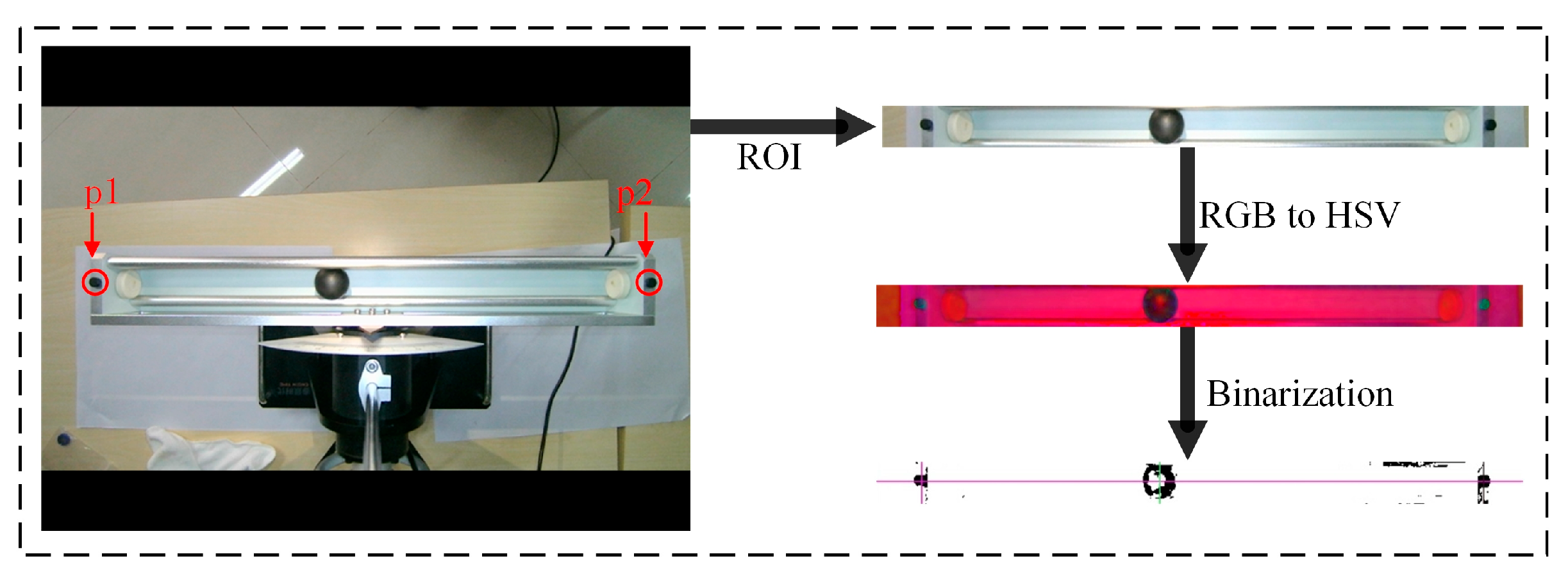
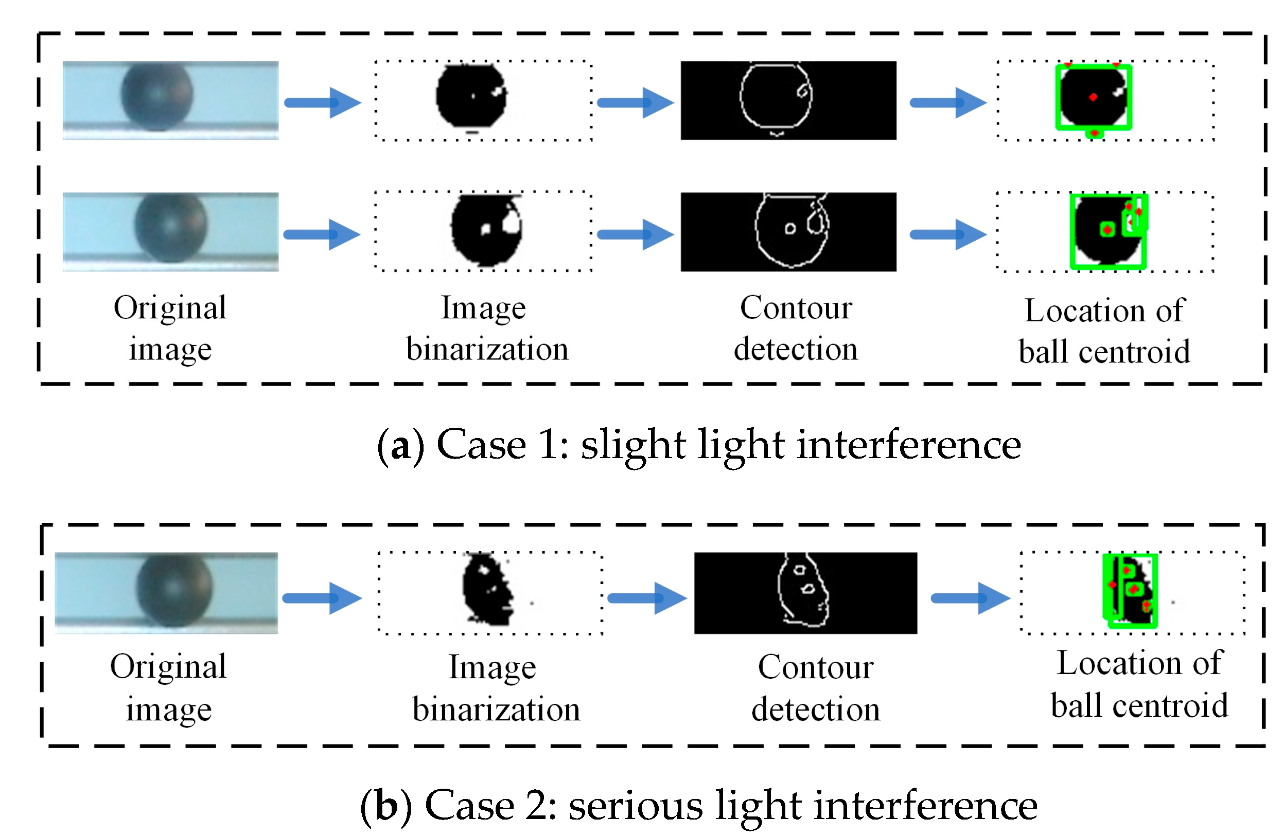
- A visual location method is proposed. When the surface features of the ball are not obvious due to the influence of the environment, the detection accuracy of this method can be improved, compared with the conventional image processing method.
- (3)
- Aiming at the limitations of the policy model trained by deep reinforcement learning in the BABS, a method of model linearization near the equilibrium point is proposed by combining nonlinear control theory and LQR theory to improve the control stability.
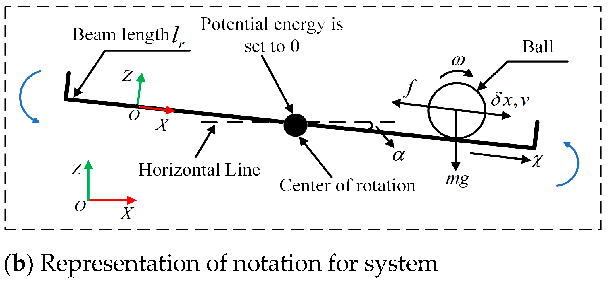
2. Dynamic Model of BABS
3. Model Design of the BABS
3.1. Control Model Design
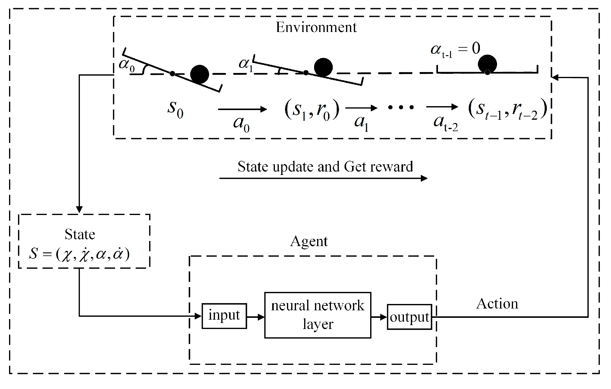
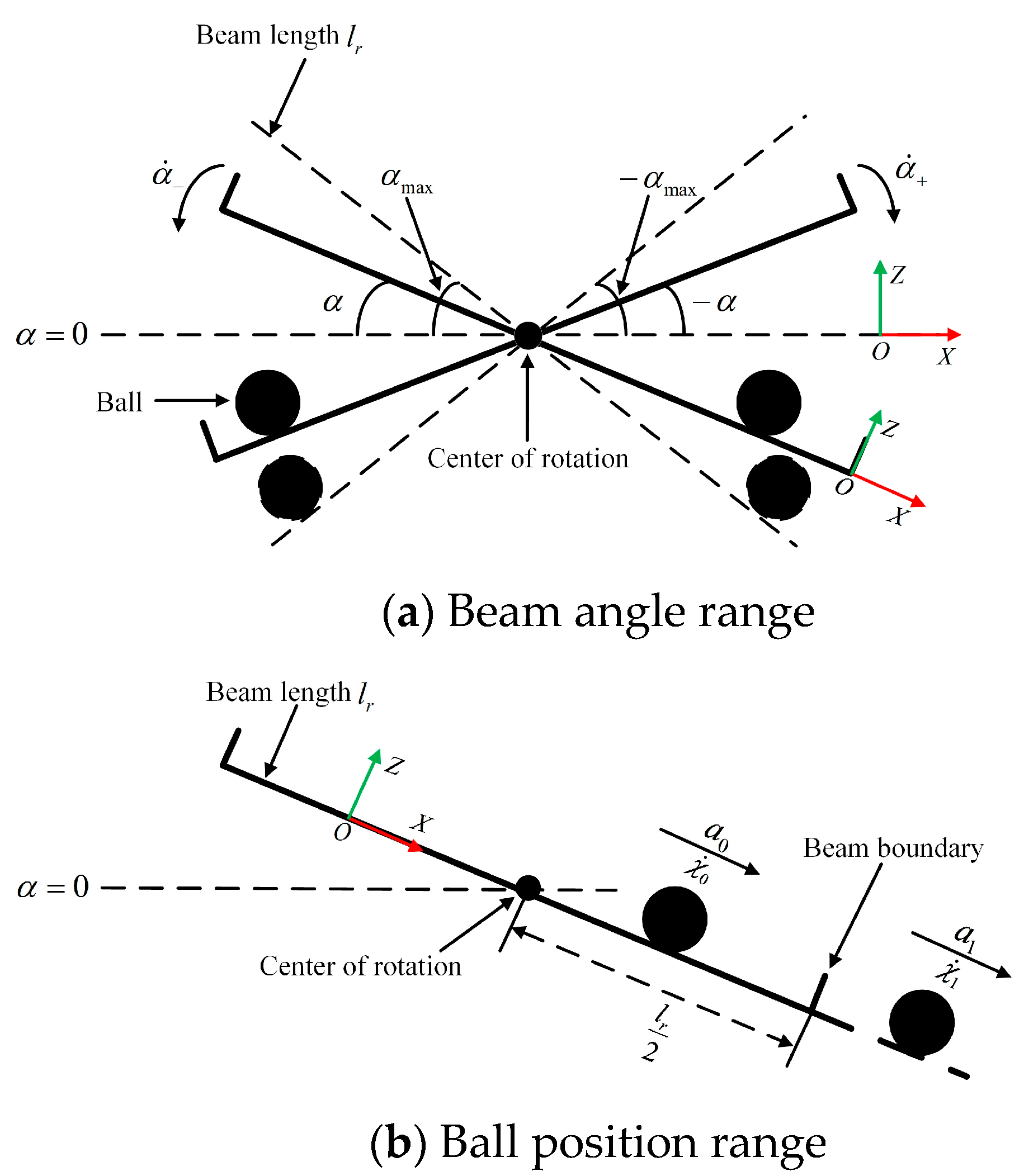
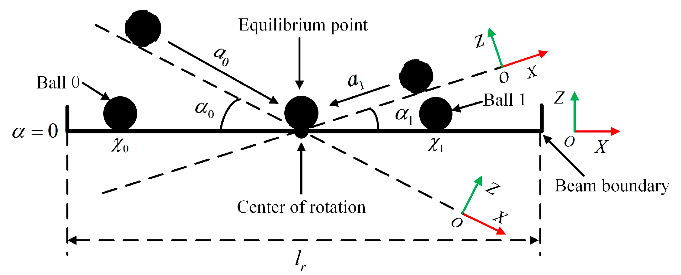
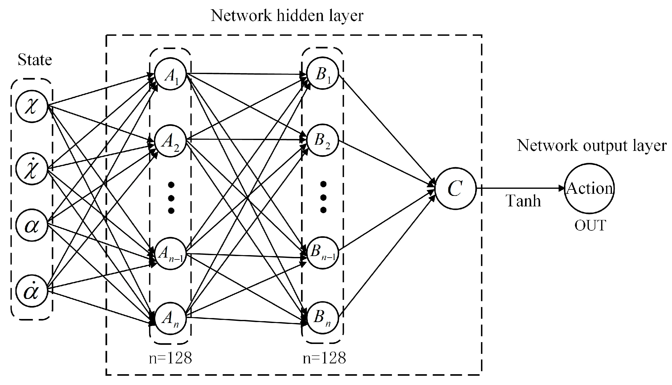
3.1.1. Reinforcement Learning Model Design
3.1.2. Detail-Reward Function
- (1)
- The evaluation function
- (2)
- The evaluation function
- (3)
- The evaluation function
3.1.3. Deep Deterministic Policy Gradient (DDPG)
| Algorithm 1: DDPG algorithm |
| Randomly initialize: critic and |
| Initialize target network , |
| Initialize replay buffer D |
| 1. For episode = 1, M do |
| 2. Initialize a random process for action exploration |
| 3. Receive initial observation state |
| 4. For t = 1, T do |
| 5. Selectn action according to the current policy and exploration noise |
| 6. Execute action and observe reward |
| 7. Store transition in D |
| 8. Sample a random minibatch of N transitions from D |
| 9. Set |
| 10. Update critic by minibatch the loss: |
| 11. Update the actor policy using the sampled gradient: |
| 12. Update the target network: |
| 13. end for |
| 14. end for |
3.2. Design of Visual Location Method
- (1)
- Planting crops: on a predetermined square land, the land is neatly divided into small plots belonging to each farmer in the row and column direction, and each farmer is planting crops on his own plot. The quantitative value of crops is denoted by variable , which satisfies . When planting crops, the quantitative value of crops is unified as .
- (2)
- Harvest crops: A farmer who was given a harvest command can harvest the crop. The rules for harvesting the crop are to first harvest the crop belonging to his plot, i.e., , then to harvest crops from adjacent plots, with the rule that the crop with a quantization value of 1 is harvested from all adjacent plots with > 0. The direction of farmers harvesting crops is from left to right, and top to bottom.
- (3)
- Counting the crop: After all harvesting instructions are completed, the farmer’s representative counts the crop. Figure 9 shows the statistical method.
4. Experiments and Results
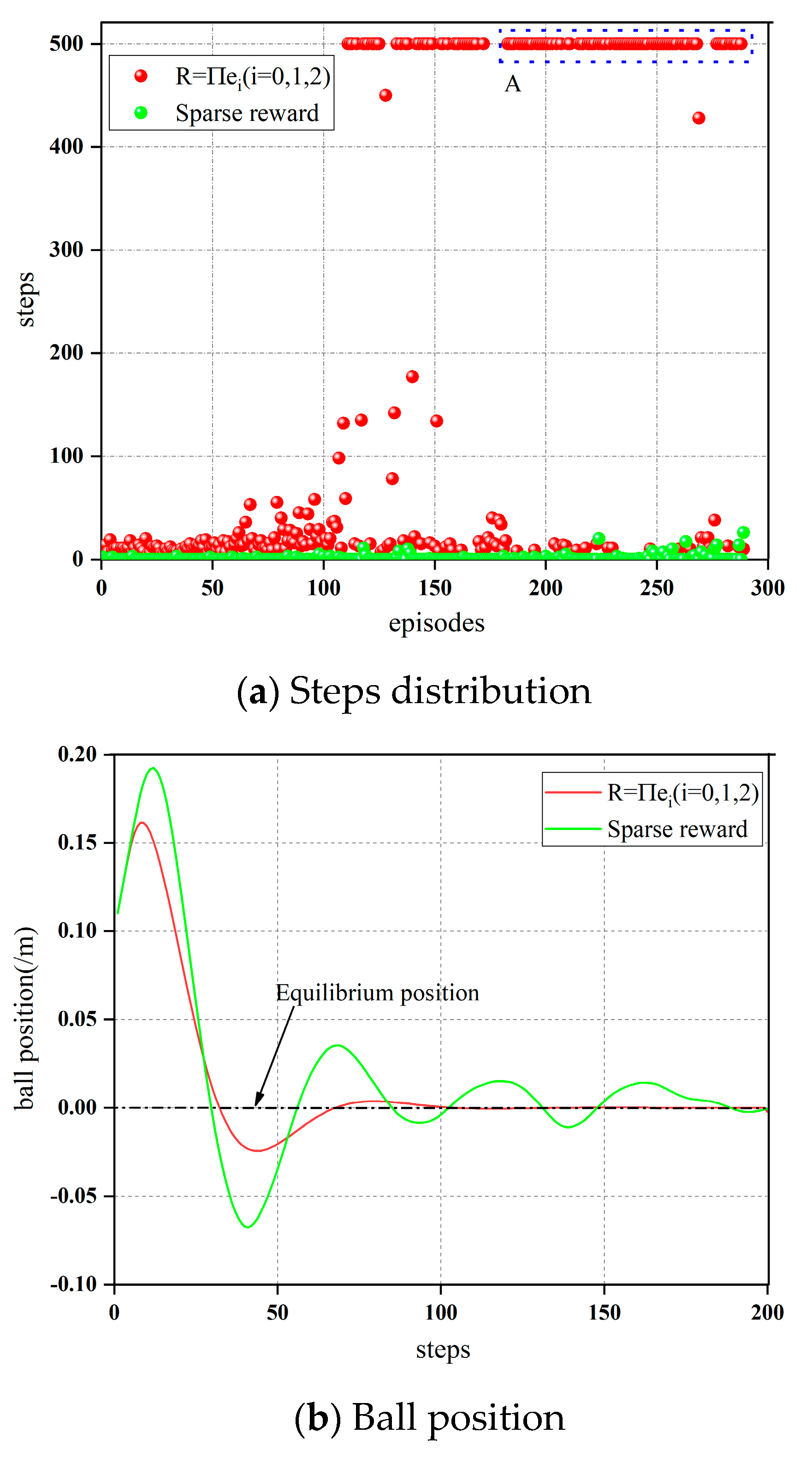
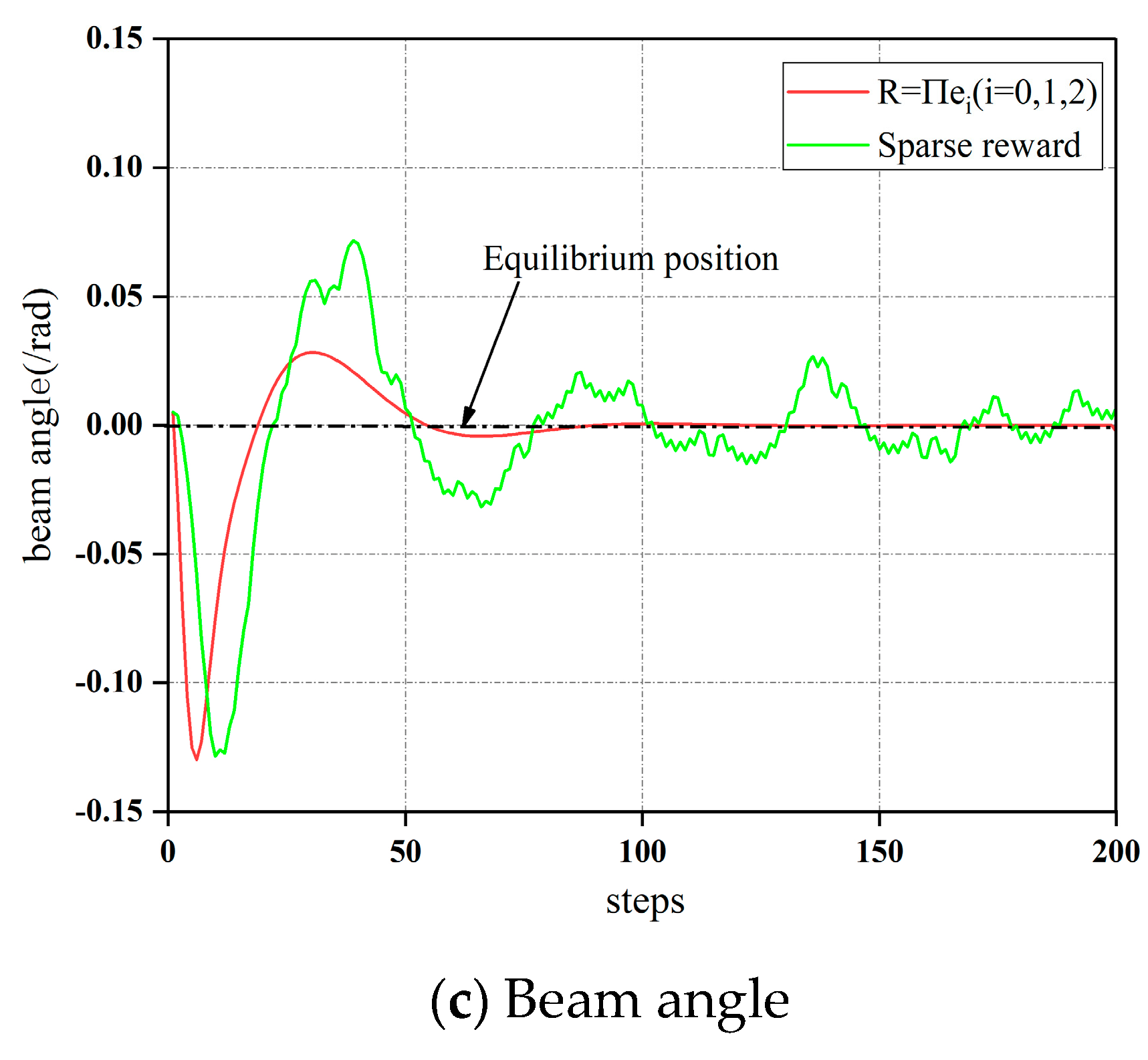
4.1. Simulation Experiment
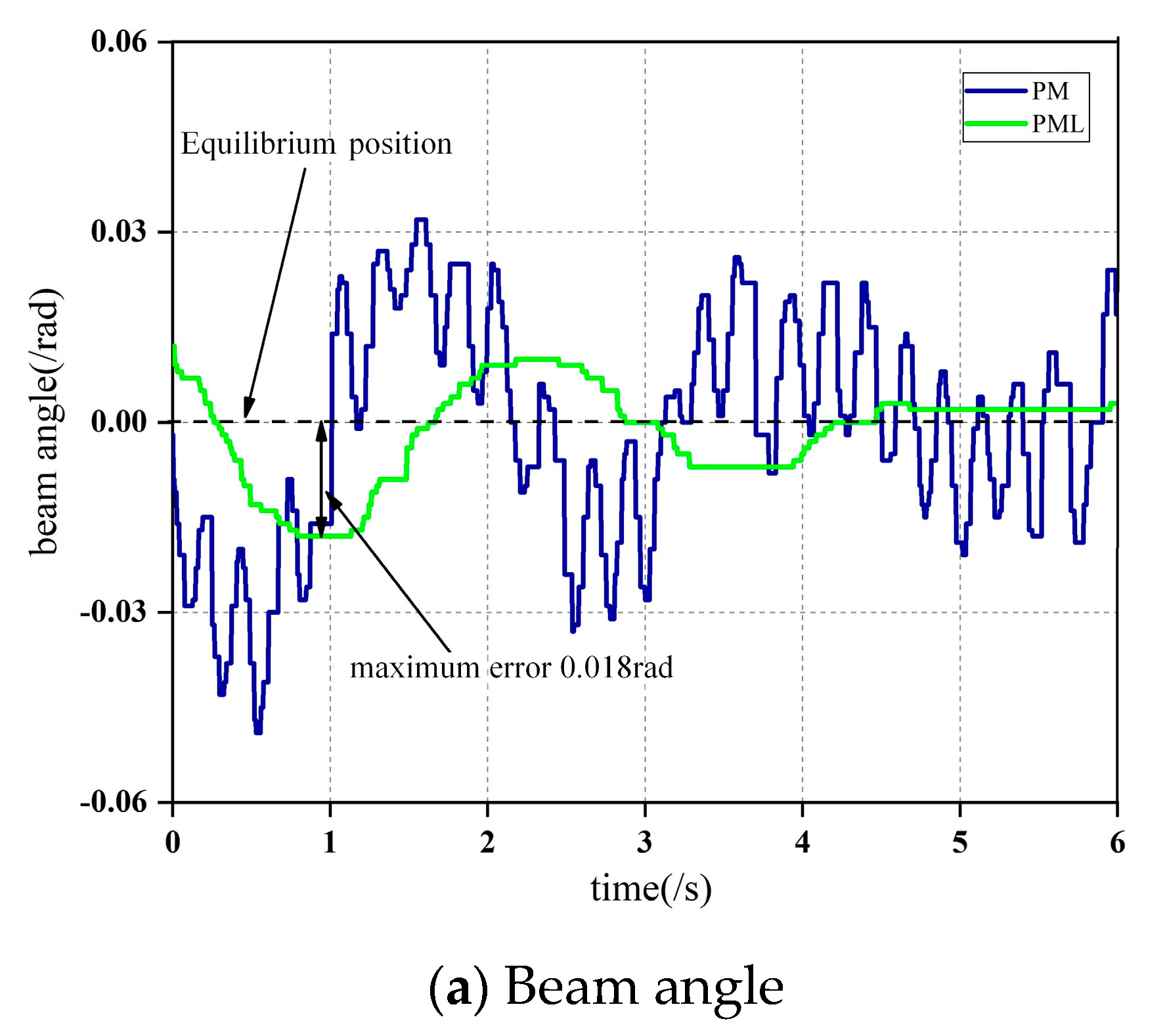
4.2. Real Platform Control Experiment
- (1)
- Observe the linear characteristics of the output value of PM produced by training in the dynamic environment near the equilibrium point in the real platform.
- (2)
- In the case of satisfactory linearity, the best linear parameters , , , are obtained by linearization.
4.3. Experimental Comparison of Different Control Methods
5. Conclusions and Future Work
Author Contributions
Funding
Institutional Review Board Statement
Informed Consent Statement
Data Availability Statement
Acknowledgments
Conflicts of Interest
References
- Murray, R.M. Future directions in control, dynamics, and systems: Overview, grand challenges, and new courses. Eur. J. Control 2003, 9, 144–158, Lavoisier and FRANCE. Available online: http://www.cds.caltech.edu/~murray/papers/2003l_mur03-ejc.html (accessed on 14 January 2003). [CrossRef]
- Bars, R.; Colaneri, P.; de Souza, C.E.; Dugard, L.; Allgöwer, F.; Kleimenov, A.; Scherer, C. Theory, algorithms and technology in the design of control systems. Annu. Rev. Control 2006, 30, 19–30. [Google Scholar] [CrossRef]
- Boubaker, O. The inverted pendulum: A fundamental benchmark in control theory and robotics. In Proceedings of the International Conference on Education and e-Learning Innovations, Sousse, Tunisia, 1–3 July 2012; IEEE: Piscataway, NJ, USA, 2012; pp. 1–6. [Google Scholar] [CrossRef]
- Andreev, F.; Auckly, D.; Gosavi, S.; Kapitanski, L.; Kelkar, A.; White, W. Matching, linear systems, and the ball and beam. Automatica 2002, 38, 2147–2152. [Google Scholar] [CrossRef]
- Aranda, J.; Chaos, D.; Dormido-Canto, S.; Muñoz, R.; Manuel Díaz, J. Benchmark control problems for a non-linear underactuated hovercraft: A simulation laboratory for control testing. IFAC Proc. Vol. 2006, 39, 463–468. [Google Scholar] [CrossRef]
- Hauser, J.; Sastry, S.; Kokotovic, P. Nonlinear control via approximate input-output linearization: The ball and beam example. IEEE Trans. Autom. Control 1992, 37, 392–398. [Google Scholar] [CrossRef]
- Nguyen, T.D.; Minh, P.V.; Phan, H.C.; Ta, D.T.; Nguyen, T.D. Bending of symmetric sandwich FGM beams with shear connectors. Math. Probl. Eng. 2021, 2021, 7596300. [Google Scholar] [CrossRef]
- Tran, T.T.; Nguyen, N.H.; Do, T.V.; Minh, P.V.; Nguyen, D.D. Bending and thermal buckling of unsymmetric functionally graded sandwich beams in high-temperature environment based on a new third-order shear deformation theory. J. Sandw. Struct. Mater. 2021, 23, 906–930. [Google Scholar] [CrossRef]
- Nam, V.H.; Vinh, P.V.; Chinh, N.V.; Do, T.V.; Hong, T.T. A new beam model for simulation of the mechanical behaviour of variable thickness functionally graded material beams based on modified first order shear deformation theory. Materials 2019, 12, 404. [Google Scholar] [CrossRef]
- Nguyen, H.N.; Hong, T.T.; Vinh, P.V.; Do, T.V. An efficient beam element based on Quasi-3D theory for static bending analysis of functionally graded beams. Materials 2019, 12, 2198. [Google Scholar] [CrossRef] [Green Version]
- Tho, N.C.; Nguyen, T.T.; To, D.T.; Minh, P.V.; Hoa, L.K. Modelling of the flexoelectric effect on rotating nanobeams with geometrical imperfection. J. Brazil. Soc. Mech. Sci. Eng. 2021, 43, 510. [Google Scholar] [CrossRef]
- Tho, N.C.; Ta, N.T.; Thom, D.V. New numerical results from simulations of beams and space frame systems with a tuned mass damper. Materials 2019, 12, 1329. [Google Scholar] [CrossRef]
- Mahmoodabadi, M.J.; Danesh, N. Gravitational search algorithm-based fuzzy control for a nonlinear ball and beam system. J. Control Decis. 2018, 5, 229–240. [Google Scholar] [CrossRef]
- Yu, W.; Ortiz, F. Stability analysis of PD regulation for ball and beam system. In Proceedings of the 2005 IEEE Conference on Control Applications, Toronto, ON, Canada, 28–31 August 2005; pp. 517–522. [Google Scholar] [CrossRef]
- Sira-Ramirez, H. On the control of the” ball and beam” system: A trajectory planning approach. In Proceedings of the 39th IEEE Conference on Decision and Control, Sydney, NSW, Australia, 12–15 December 2000; Volume 4, pp. 4042–4047. [Google Scholar] [CrossRef]
- Almutairi, N.B.; Zribi, M. On the sliding mode control of a ball on a beam system. Nonlinear Dyn. 2010, 59, 221–238. [Google Scholar] [CrossRef]
- Friedland, B. Control System Design: An Introduction to State-Space Methods; Courier Corporation: Chicago, IL, USA, 2012. [Google Scholar]
- Danilo, M.O.; Gil-González, W.; Ramírez-Vanegas, C. Discrete-inverse optimal control applied to the ball and beam dynamical system: A passivity-based control approach. Symmetry 2020, 12, 1359. [Google Scholar] [CrossRef]
- Ho, M.T.; Rizal, Y.; Chu, L.M. Visual servoing tracking control of a ball and plate system: Design, implementation and experimental validation. Int. J. Adv. Robot. Syst. 2013, 10, 287. [Google Scholar] [CrossRef]
- Moreno-Armendariz, M.A.; Pérez-Olvera, C.A.; Rodríguez, F.O.; Rubio, E. Indirect hierarchical FCMAC control for the ball and plate system. Neurocomputing 2010, 73, 2454–2463. [Google Scholar] [CrossRef]
- Yuan, D.; Zhang, Z. Modelling and control scheme of the ball–plate trajectory-tracking pneumatic system with a touch screen and a rotary cylinder. IET Control Theory Appl. 2010, 4, 573–589. [Google Scholar] [CrossRef]
- Mehedi, I.M.; Al-Saggaf, U.M.; Mansouri, R.; Bettayeb, M. Two degrees of freedom fractional controller design: Application to the ball and beam system. Measurement 2019, 135, 13–22. [Google Scholar] [CrossRef]
- Meenakshipriya, B.; Kalpana, K. Modelling and control of ball and beam system using coefficient diagram method (CDM) based PID controller. IFAC Proc. 2014, 47, 620–626. [Google Scholar] [CrossRef]
- Márton, L.; Hodel, A.S.; Lantos, B.; Hung, J.Y. Underactuated robot control: Comparing LQR, subspace stabilization, and combined error metric approaches. IEEE Trans. Ind. Electron. 2008, 55, 3724–3730. [Google Scholar] [CrossRef]
- Keshmiri, M.; Jahromi, A.F.; Mohebbi, A.; Amoozgar, M.H.; Xie, W.F. Modeling and control of ball and beam system using model based and non-model based control approaches. Int. J. Smart Sens. Intell. Syst. 2017, 5, 14–35. [Google Scholar] [CrossRef]
- Choudhary, M.K.; Kumar, G.N. ESO based LQR controller for ball and beam system. IFAC-Pap. 2016, 49, 607–610. [Google Scholar] [CrossRef]
- da Silveira Castro, R.; Flores, J.V.; Salton, A.T. A comparative analysis of repetitive and resonant controllers to a servo-vision ball and plate system. IFAC Proc. 2014, 47, 1120–1125. [Google Scholar] [CrossRef]
- Chang, Y.H.; Chan, W.S.; Chang, C.W.; Tao, C.W. Adaptive fuzzy dynamic surface control for ball and beam system. Int. J. Fuzzy Syst. 2011, 13, 1–7. [Google Scholar]
- Chien, T.L.; Chen, C.C.; Tsai, M.C.; Chen, Y.C. Control of AMIRA’s ball and beam system via improved fuzzy feedback linearization approach. Appl. Math. Model. 2010, 34, 3791–3804. [Google Scholar] [CrossRef]
- Castillo, O.; Lizárraga, E.; Soria, J.; Melin, P.; Valdez, F. New approach using ant colony optimization with ant set partition for fuzzy control design applied to the ball and beam system. Inf. Sci. 2015, 294, 203–215. [Google Scholar] [CrossRef]
- Chang, Y.H.; Chang, C.W.; Tao, C.W.; Lin, H.W.; Taur, J.S. Fuzzy sliding-mode control for ball and beam system with fuzzy ant colony optimization. Expert Syst. Appl. 2012, 39, 3624–3633. [Google Scholar] [CrossRef]
- Hammadih, M.L.; Hosani, K.A.; Boiko, I. Interpolating sliding mode observer for a ball and beam system. Int. J. Control 2016, 89, 1879–1889. [Google Scholar] [CrossRef]
- Hung, L.C.; Chung, H.Y. Decoupled control using neural network-based sliding-mode controller for nonlinear systems. Expert Systems with Applications. 2007, 32, 1168–1182. [Google Scholar] [CrossRef]
- Das, A.; Roy, P. Improved performance of cascaded fractional-order SMC over cascaded SMC for position control of a ball and plate system. IETE J. Res. 2017, 63, 238–247. [Google Scholar] [CrossRef]
- Singh, R.; Bhushan, B. Real-time control of ball balancer using neural integrated fuzzy controller. Artif. Intell. Rev. 2020, 53, 351–368. [Google Scholar] [CrossRef]
- Zhang, L.; Chen, W.; Wang, J.; Zhang, J. Adaptive robust slide mode trajectory tracking controller for lower extremity rehabilitation exoskeleton. In Proceedings of the 2018 13th IEEE Conference on Industrial Electronics and Applications (ICIEA), Wuhan, China, 31 May–2 June 2018; IEEE: Piscataway, NJ, USA, 2018; pp. 992–997. [Google Scholar] [CrossRef]
- Wang, F.Y.; Zhang, H.; Liu, D. Adaptive dynamic programming: An introduction. IEEE Comput. Intell. Mag. 2009, 4, 39–47. [Google Scholar] [CrossRef]
- Mu, C.; Zhang, Y.; Gao, Z.; Sun, C. ADP-based robust tracking control for a class of nonlinear systems with unmatched uncertainties. IEEE Trans. Syst. Man Cybern. Syst. 2019, 50, 4056–4067. [Google Scholar] [CrossRef]
- Dong, H.; Zhao, X.; Luo, B. Optimal tracking control for uncertain nonlinear systems with prescribed performance via critic-only adp. IEEE Trans. Syst. Man Cybern. Syst. 2020, 52, 561–573. [Google Scholar] [CrossRef]
- Song, R.; Zhu, L. Optimal fixed-point tracking control for discrete-time nonlinear systems via ADP. IEEE/CAA J. Autom. Sin. 2019, 6, 657–666. [Google Scholar] [CrossRef]
- Ni, Z.; He, H.; Zhao, D.; Xu, X.; Prokhorov, D.V. GrDHP: A general utility function representation for dual heuristic dynamic programming. IEEE Trans. Neural Netw. Learn. Syst. 2014, 26, 614–627. [Google Scholar] [CrossRef]
- Song, R.; Wei, Q.; Sun, Q. Nearly finite-horizon optimal control for a class of nonaffine time-delay nonlinear systems based on adaptive dynamic programming. Neurocomputing 2015, 156, 166–175. [Google Scholar] [CrossRef]
- Burghardt, A.; Szuster, M. Neuro-dynamic programming in control of the ball and beam system. In Solid State Phenomena; Trans Tech Publications Ltd.: Wollerau, Switzerland, 2014; Volume 210, pp. 206–214. [Google Scholar] [CrossRef]
- Thorndike, E.L. Animal intelligence: An experimental study of the associative processes in animals. Psychol. Rev. Monogr. Suppl. 1898, 2, 149. [Google Scholar] [CrossRef]
- Watkins, C.J.C.H.; Dayan, P. Q-learning. Mach. Learn. 1992, 8, 279–292. [Google Scholar] [CrossRef]
- Jin, Z.; Liu, A.; Zhang, W.A.; Yu, L.; Su, C.Y. A Learning Based Hierarchical Control Framework for Human-Robot Collaboration. IEEE Trans. Autom. Sci. Eng. 2022, 1–12. [Google Scholar] [CrossRef]
- Zhong, X.; Ni, Z.; He, H. Gr-GDHP: A new architecture for globalized dual heuristic dynamic programming. IEEE Trans. Cybern. 2016, 47, 3318–3330. [Google Scholar] [CrossRef]
- Ni, Z.; He, H.; Zhong, X.; Prokhorov, D.V. Model-free dual heuristic dynamic programming. IEEE Trans. Neural Netw. Learn. Syst. 2015, 26, 1834–1839. [Google Scholar] [CrossRef]
- Ganesh, A.; Sundareswari, M.B.; Panda, M.; Mozhi, G.T.; Dhanalakshmi, K. Reinforcement learning control of servo actuated centrally pivoted ball on a beam. In Proceedings of the 2020 IEEE 15th International Conference on Industrial and Information Systems (ICIIS), Rupnagar, India, 26–28 November 2020; pp. 103–108. [Google Scholar] [CrossRef]
- Yao, S.; Liu, X.; Zhang, Y.; Cui, Z. An approach to solving optimal control problems of nonlinear systems by introducing detail-reward mechanism in deep reinforcement learning. Math. Biosci. Eng. 2022, 19, 9258–9290. [Google Scholar] [CrossRef]
- Ryu, K.; Oh, Y. Balance control of ball-beam system using redundant manipulator. In Proceedings of the 2011 IEEE International Conference on Mechatronics, Istanbul, Turkey, 13–15 April 2011; pp. 403–408. [Google Scholar] [CrossRef]
- Liu, T.; Wang, N.; Zhang, L.; Ai, S.M.; Du, H.W. A novel visual measurement method for three-dimensional trajectory of underwater moving objects based on deep learning. IEEE Access 2020, 8, 186376–186392. [Google Scholar] [CrossRef]
- Supreeth, H.S.G.; Patil, C.M. Moving object detection and tracking using deep learning neural network and correlation filter. In Proceedings of the 2018 Second International Conference on Inventive Communication and Computational Technologies (ICICCT), Coimbatore, India, 20–21 April 2018; IEEE: Piscataway, NJ, USA, 2018; pp. 1775–1780. [Google Scholar] [CrossRef]
- Pathak, A.R.; Pandey, M.; Rautaray, S. Application of deep learning for object detection. Procedia Comput. Sci. 2018, 132, 1706–1717. [Google Scholar] [CrossRef]
- Mukherjee, M.; Potdar, Y.U.; Potdar, A.U. Object tracking using edge detection. In Proceedings of the International Conference and Workshop on Emerging Trends in Technology, Maharashtra, India, 26–27 February 2010; pp. 686–689. [Google Scholar] [CrossRef]
- Qul’am, H.M.; Dewi, T.; Risma, P.; Oktarina, Y.; Permatasari, D. Edge detection for online image processing of a vision guide pick and place robot. In Proceedings of the 2019 International Conference on Electrical Engineering and Computer Science (ICECOS), Batam, Indonesia, 2–3 October 2019; IEEE: Piscataway, NJ, USA, 2019; pp. 102–106. [Google Scholar] [CrossRef]
- Wang, B.; Zhang, K.; Shi, L.; Zhong, H.H. An edge detection algorithm of moving object based on background modeling and active contour model. In Advanced Materials Research; Trans Tech Publications Ltd.: Wollerau, Switzerland, 2013; Volume 765, pp. 2393–2398. [Google Scholar] [CrossRef]
- Suzuki, S. Topological structural analysis of digitized binary images by border following. Comput. Vis. Graph. Image Process. 1985, 30, 32–46. [Google Scholar] [CrossRef]
- Sutton, R.S.; Barto, A.G. Reinforcement Learning: An Introduction; MIT Press: Cambridge, MA, USA, 1998; Volume 1. [Google Scholar]
- Vecerik, M.; Hester, T.; Scholz, J.; Wang, F.; Pietauin, O.; Piot, B.; Heess, N.; Rothörl, T.; Lampe, T.; Riedmiller, M. Leveraging demonstrations for deep reinforcement learning on robotics problems with sparse rewards. arXiv 2017, arXiv:1707.08817. [Google Scholar] [CrossRef]
- Ng, A.Y.; Harada, D.; Russell, S. Policy invariance under reward transformations: Theory and application to reward shaping. Icml 1999, 99, 278–287. [Google Scholar]
- Zhu, Y.; Zhao, D.; He, H. Integration of fuzzy controller with adaptive dynamic programming. In Proceedings of the 10th World Congress on Intelligent Control and Automation, Beijing, China, 6–8 July 2012; IEEE: Piscataway, NJ, USA, 2012; pp. 310–315. [Google Scholar] [CrossRef]
- Wang, Z.Y.; Dai, Y.P.; Li, Y.W.; Yao, Y. A kind of utility function in adaptive dynamic programming for inverted pendulum control. In Proceedings of the 2010 International Conference on Machine Learning and Cybernetics, Qingdao, China, 11–14 July 2010; IEEE: Piscataway, NJ, USA, 2010; Volume 3, pp. 1538–1543. [Google Scholar] [CrossRef]
- Lillicrap, T.P.; Hunt, J.J.; Pritzel, A.; Heess, N.; Erez, T.; Tassa, Y.; Silver, D.; Wierstra, D. Continuous control with deep reinforcement learning. arXiv 2015, arXiv:1509.02971. [Google Scholar] [CrossRef]
- Satheeshbabu, S.; Uppalapati, N.K.; Fu, T.; Krishnan, G. Continuous control of a soft continuum arm using deep reinforcement learning. In Proceedings of the 2020 3rd IEEE International Conference on Soft Robotics (RoboSoft), New Haven, CT, USA, 15 May–15 July 2020; IEEE: Piscataway, NJ, USA, 2020; pp. 497–503. [Google Scholar] [CrossRef]
- Ma, Y.; Zhu, W.; Benton, M.G.; Romagnoli, J. Continuous control of a polymerization system with deep reinforcement learning. J. Process Control 2019, 75, 40–47. [Google Scholar] [CrossRef]
- Nwankpa, C.; Ijomah, W.; Gachagan, A.; Marshall, S. Activation functions: Comparison of trends in practice and research for deep learning. arXiv 2018, arXiv:1811.03378. [Google Scholar] [CrossRef]
- Chaudhuri, D.; Samal, A. A simple method for fitting of bounding rectangle to closed regions. Pattern Recognit. 2007, 40, 1981–1989. [Google Scholar] [CrossRef]
- Vukic, Z. Nonlinear Control Systems; CRC Press: Boca Raton, FL, USA, 2003. [Google Scholar]


| Network | Network Structure | Loss Function | Activate Function | Optimization Function | Batch Size | |
|---|---|---|---|---|---|---|
| Actor | (4,128) (128,128) (128,1) | 1 × 10⁻³ | Relu | Adam | 64 | |
| Critic | (5,128) (128,128) (128,1) | 1 × 10⁻² | MSE | Relu | Adam | 64 |
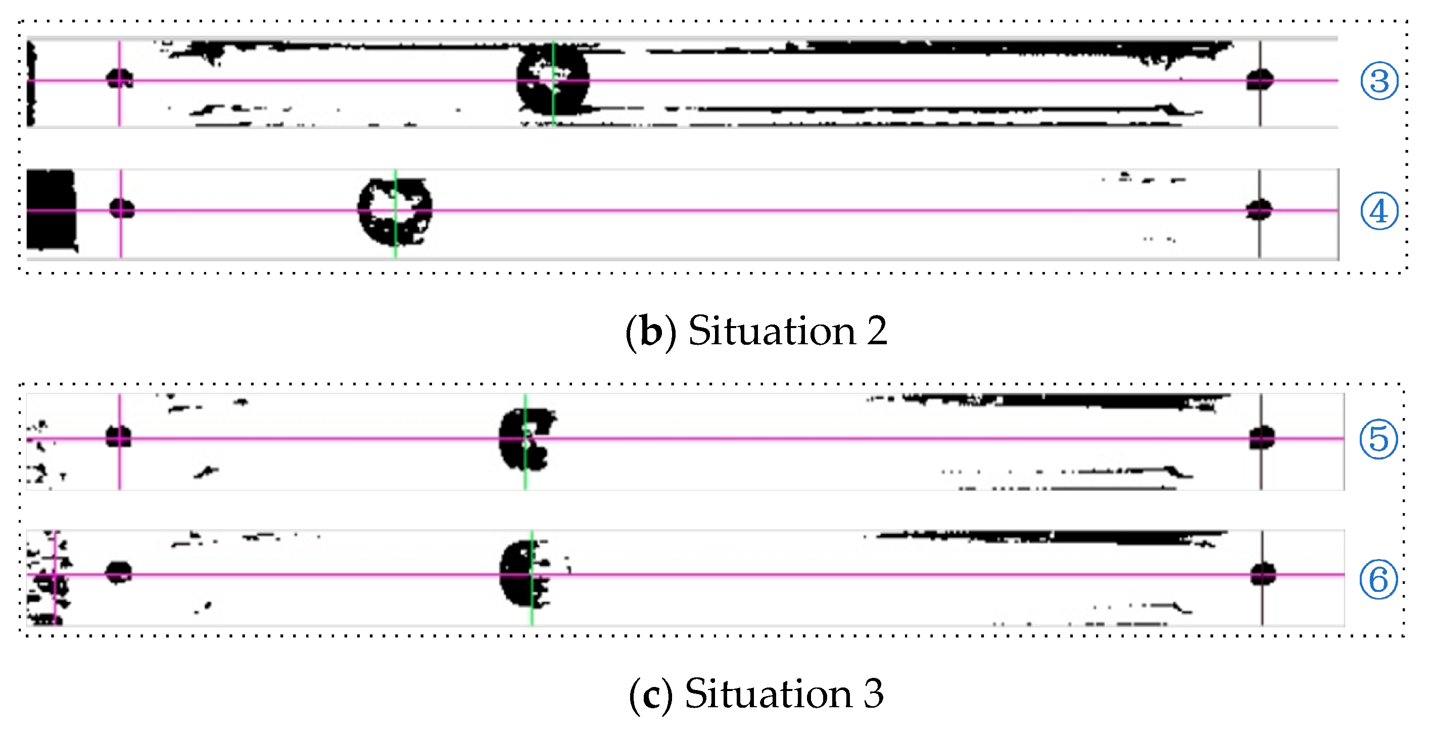
| No. | ① | ② | ③ | ④ | ⑤ | ⑥ |
|---|---|---|---|---|---|---|
| Actual pixel coordinates | (387,21) | (316,23) | (316,23) | (222,22) | (301,22) | (301,22) |
| Location pixel coordinates | (387,24) | (318,23) | (317,24) | (222,24) | (299,24) | (303,24) |
| Episodes | Steps | Discount Factor | Memory | |
|---|---|---|---|---|
| 500 | 500 | 0.99 | 1 × 10⁻² | 10,000 |
| Experimental Phases | Ball Position (/m) | Ball Velocity (m/s) | Beam Angle (/rad) | Beam Angular Velocity (rad/s) |
|---|---|---|---|---|
| Training phase | (−0.16,0.16) | (−0.08,0.08) | (−0.209,0.209) | (−0.05,0.05) |
| Testing phase | 0.11 | 0.2 | 0.005 | −0.177 |
| Moment of Inertia | ||||
|---|---|---|---|---|
| 0.113 kg | 0.015 m | 0.4 m | 0.00001017 kgm2 | 9.8 m/s2 |
Publisher’s Note: MDPI stays neutral with regard to jurisdictional claims in published maps and institutional affiliations. |
© 2022 by the authors. Licensee MDPI, Basel, Switzerland. This article is an open access article distributed under the terms and conditions of the Creative Commons Attribution (CC BY) license (https://creativecommons.org/licenses/by/4.0/).
Share and Cite
Yao, S.; Liu, X.; Zhang, Y.; Cui, Z. Research on Solving Nonlinear Problem of Ball and Beam System by Introducing Detail-Reward Function. Symmetry 2022, 14, 1883. https://doi.org/10.3390/sym14091883
Yao S, Liu X, Zhang Y, Cui Z. Research on Solving Nonlinear Problem of Ball and Beam System by Introducing Detail-Reward Function. Symmetry. 2022; 14(9):1883. https://doi.org/10.3390/sym14091883
Chicago/Turabian StyleYao, Shixuan, Xiaochen Liu, Yinghui Zhang, and Ze Cui. 2022. "Research on Solving Nonlinear Problem of Ball and Beam System by Introducing Detail-Reward Function" Symmetry 14, no. 9: 1883. https://doi.org/10.3390/sym14091883
APA StyleYao, S., Liu, X., Zhang, Y., & Cui, Z. (2022). Research on Solving Nonlinear Problem of Ball and Beam System by Introducing Detail-Reward Function. Symmetry, 14(9), 1883. https://doi.org/10.3390/sym14091883